
Abstract
Criteria are established for existence of least one or three positive solutions for boundary value problems of second-order functional dynamic equations on time scales. By this purpose, we use a fixed-point index theorem in cones and Leggett-Williams fixed-point theorem.
1. Introduction
In a recent paper [1], by applying a fixed-point index theorem in cones, Jiang and Weng studied the existence of positive solutions for the boundary value problems described by second-order functional differential equations of the form

Aykut [2] applied a cone fixed-point index theorem in cones and obtained sufficient conditions for the existence of positive solutions of the boundary value problems of functional difference equations of the form

In this article, we are interested in proving the existence and multiplicity of positive solutions for the boundary value problems of a second-order functional dynamic equation of the form

Throughout this paper we let  be any time scale (nonempty closed subset of
  ) and
) and  be a subset of
  such that
  and for
  is not right scattered and left dense at the same time.
Some preliminary definitions and theorems on time scales can be found in books [3, 4] which are excellent references for calculus of time scales.
We will assume that the following conditions are satisfied.
(H1) 
(H2)  is continuous with respect to
  and
and  for
for  , where
  denotes the set of nonnegative real numbers.
(H3)  defined on
  satisfies

Let  be nonempty subset of

(H4) 
if  then
then  ;
;  for
for  , where
  denotes the set of all positively regressive and rd-continuous functions.
(H5)  and
and  are defined on
  and
and  , respectively, where
 ; furthermore,
  ;
;

There have been a number of works concerning of at least one and multiple positive solutions for boundary value problems recent years. Some authors have studied the problem for ordinary differential equations, while others have studied the problem for difference equations, while still others have considered the problem for dynamic equations on a time scale [5–10]. However there are fewer research for the existence of positive solutions of the boundary value problems of functional differential, difference, and dynamic equations [1, 2, 11–13].
Our problem is a dynamic analog of the BVPs (1.1) and (1.2). But it is more general than them. Moreover, conditions for the existence of at least one positive solution were studied for the BVPs (1.1) and (1.2). In this paper, we investigate the conditions for the existence of at least one or three positive solutions for the BVP (1.3). The key tools in our approach are the following fixed-point index theorem [14], and Leggett-Williams fixed-point theorem [15].
Theorem 1.1 (see [14]).
Let  be Banach space and
  be a cone in
  . Let
. Let  , and define
  . Assume
  is a completely continuous operator such that
  for
for 
-
(i)
If
 for
for  , then
-
(ii)
If
 for
for  , then
 for
for  , then
 for
for  , then
Theorem 1.2 (see [15]).
Let be a cone in the real Banach space
  . Set
. Set

Suppose that  is a completely continuous operator and
  is a nonnegative continuous concave functional on
  with
with  for all
  . If there exists
  such that the following conditions hold:
-
(i)
 and
and  for all
-
(ii)
 for
for 
-
(iii)
 for
for  with
with 
 and
and  for all
 for
for 
 for
for  with
with 
Then  has at least three fixed points
  in
in  satisfying

2. Preliminaries
First, we give the following definitions of solution and positive solution of BVP (1.3).
Definition 2.1.
We say a function  is a solution of BVP (1.3) if it satisfies the following.
-
(1)
 is nonnegative on
  .
. -
(2)
 as
as  , where
  is defined as
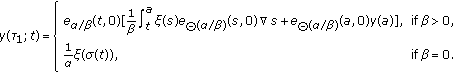 (21)
(21) -
(3)
 as
as  , where
  is defined as
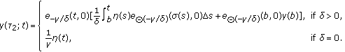 (22)
(22) -
(4)
 is
is  -differentiable,
  is
is  -differentiable on
  and
and  is continuous.
 -
(5)
 for
for 
 is nonnegative on
  .
. as
as  , where
  is defined as
 as
as  , where
  is defined as
 is
is  -differentiable,
  is
is  -differentiable on
  and
and  is continuous.
 for
for 
Furthermore, a solution  of (1.3) is called a positive solution if
  for
for 
Denote by  and
and  the solutions of the corresponding homogeneous equation

under the initial conditions

Set

Since the Wronskian of any two solutions of (2.3) is independent of  , evaluating at
  and using the initial conditions (2.4) yield

Using the initial conditions (2.4), we can deduce from (2.3) for  and
and  , the following equations:


(See [8].)
Lemma 2.2 (see [8]).
Under the conditions (H1) and the first part of (H4) the solutions  and
and  possess the following properties:

Let  be the Green function for the boundary value problem:

given by

where  and
and  are given in (2.7) and (2.8), respectively. It is obvious from (2.6), (H1) and (H4), that
  holds.
Lemma 2.3.
Assume the conditions (H1) and (H4) are satisfied. Then
-
(i)
 for
for 
-
(ii)
 for
for  and
and 
 for
for 
 for
for  and
and 
where

in which

Proof.
 for
for  , and
, and  , for
, for  . Besides,
  is nondecreasing and
  is nonincreasing, for
  . Therefore, we have

So statement (i) of the lemma is proved. If  for a given
  then statement (ii) of the lemma is obvious for such values. Now,
  and
and  . Consequently,
  , for all such
  Let us take any
  . Then we have for
  ,
,

and we have for  ,
,

Let  be endowed with maximum norm
  for
for  , and let
  be a cone defined by

where  is as in (2.12).
Suppose that  is a solution of (1.3), then it can be written as

where

Throughout this paper we assume that  is the solution of (1.3) with
  . Clearly,
  can be expressed as follows:

where

Let  be a solution of (1.3) and
  . Noting that
  for
for  , we have

where

Define an operator  as follows:

where

It is easy to derive that  is a positive solution of BVP (1.3) if and only if
  is a nontrivial fixed point
  of
of  , where
  be defined as before.
Lemma 2.4.

Proof.
For  , we have
  . Moreover, we have from definition of
  that
that  and
and  , for
, for  and
and  , respectively. Thus,
  where
where  . It follows from the definition
  and Lemma 2.3 that

Thus,  .
.
Lemma 2.5.
 is completely continuous.
Lemma 2.6.
If

for all  , then there exist
  such that
  , for
, for  and
and  , for
, for  .
.
Proof.
Choose  such that

By using the first equality of (2.27), we can choose  such that

If  , then for
  , we have

Therefore we get

Thus, we have from Theorem 1.1,  , for
, for  . On the other hand, the second equality of (2.27) implies for every
  , there is an
  , such that

Here we choose  satisfying (2.28). For
  , we have definition of
  that
that

It follows from (2.32) that

This shows that

Thus, by Theorem 1.1, we conclude that  for
for  . The proof is therefore complete.
3. Existence of One Positive Solution
In this section, we investigate the conditions for the existence of at least one positive solution of the BVP (1.3).
In the next theorem, we will also assume that the following condition on  .
.
(H6):

where  is large enough such that

and  is small enough such that

where  is the eigenfunction related to the smallest eigenvalue
  of the eigenvalue problem:

Theorem 3.1.
If (H1)–(H6) are satisfied, then the BVP (1.3) has at least one positive solution.
Proof.
Fix  and let
  for
for  . Then,
  satisfies (2.27). Define
  by
by

where

Then  is a completely continuous operator. One has from Lemma 2.6 that there exist
  such that


Define  by
by  then
then  is a completely continuous operator. By the first equality in (H6) and the definition of
  , there are
  and
and  such that

We now prove that  for all
  and
and  . In fact, if there exists
  and
and  such that
  , then
  satisfies the equation

and the boundary conditions

Multiplying both sides of (3.10) by  , then integrating from
  to
to  , and using integration by parts in the left-hand side two times, we obtain

Combining (3.9) and (3.12), we get

We also have

Equations (3.13) and (3.14) lead to

This is impossible. Thus  for
for  and
and  . By (3.7) and the homotopy invariance of the fixed-point index (see [11]), we get that

On the other hand, according to the second inequality of (H6), there exist  and
and  such that

We define

then it follows that

Define  by
by  , then
  is a completely continuous operator. We claim that there exists
  such that

In fact, if  for some
  and
and  , then


where  Combining (3.21) with (3.22), we have

Let  Then we get

Consequently, by the homotopy invariance of the fixed-point index, we have

where  is zero operator. Use (3.16) and (3.25) to conclude that

Hence,  has a fixed point in
  .
.
Let  . Since
  for
for  and
and  .
.
(H7)

Theorem 3.2.
If (H1)–(H5) and (H7) are satisfied, then the BVP (1.3) has at least one positive solution.
Proof.
Define  by
by  , then
  is a completely continuous operator. By the first inequality in (H7), there exist
  and
and  such that

We claim that  for
for  and
and  . In fact, if there exist
  and
and  such that
  , then
  satisfies the boundary condition (3.11). Since
  , we have
  . Then we have

Multiplying the last equation by  integrating from
  to
to  , by (3.28), we obtain

then we have

Equations (3.30) and (3.31) lead to

This is impossible. By homotopy invariance of the fixed-point index, we get that

Define  by
by  , then
  is a completely continuous operator. By the second inequality in (H7), and definition of
  , there exist
  and
and  such that

We define

then, it is obvious that

We claim that there exists  such that

In fact, if  for some
  and
and  , then using (3.36), it is analogous to the argument of (3.13) and (3.14) that

Equation (3.38) leads to  Let
Let  . Then we get

Consequently, by (3.8) and the homotopy invariance of the fixed-point index, we have

In view of (3.33) and (3.40), we obtain

Therefore,  has a fixed point in
  . The proof is completed.
Corollary 3.3.
Using the following (H8) or (H9) instead of (H6) or (H7), the conclusions of Theorems 3.1 and 3.2 are true. For  ,
,
(H8)

(H9)

4. Existence of Three Positive Solutions
In this section, using Theorem 1.2 (the Leggett-Williams fixed-point theorem) we prove the existence of at least three positive solutions to the BVP (1.3).
Define the continuous concave functional  to be
to be  , and the constants


Theorem 4.1.
Suppose there exists constants  such that
(D1)  for
for 

(D2)  for
for 

(D3) one of the following is satisfied:
-
(a)

-
(b)
there exists a constant
 such that
  for
for  and
and  ,
,

 such that
  for
for  and
and  ,
,where  ,
,  , and
, and  are as defined in (2.12), (4.1), (4.2), respectively. Then the boundary value problem (1.3) has at least three positive solutions
  and
and  satisfying

Proof.
The technique here similar to that used in [5] Again the cone  , the operator
  is the same as in the previous sections. For all
  we have
  If
If  , then
  and the condition (a) of (D3) imply that

Thus there exist a  and
and  such that if
  , then
  . For
. For  , we have
  for all
  , for all
  Pick any

Then  implies that

Thus 
The condition (b) of (D3) implies that there exists a positive number  such that
  for
for  and
and  . If
. If  , then

Thus  Consequently, the assumption (D3) holds, then there exist a number
  such that
  and
and 
The remaining conditions of Theorem 1.2 will now be shown to be satisfied.
By (D1) and argument above, we can get that  Hence, condition (ii) of Theorem 1.2 is satisfied.
We now consider condition (i) of Theorem 1.2. Choose  for
for  , where
  . Then
  and
and  so that
  . For
. For  , we have
  ,
,  . Combining with (D2), we get

for  . Thus, we have

As a result,  yields
Lastly, we consider Theorem 1.2(iii). Recall that  . If
. If  and
and  , then

Thus, all conditions of Theorem 1.2 are satisfied. It implies that the TPBVP (1.3) has at least three positive solutions  with
with

5. Examples
Example 5.1.
Let  Consider the BVP:

Then  and
and

Since  ,
,  . It is clear that (H1)–(H5) and (H8) are satisfied. Thus, by Corollary 3.3, the BVP (5.1) has at least one positive solution.
Example 5.2.
Let us introduce an example to illustrate the usage of Theorem 4.1. Let

Consider the TPBVP:

Then  and
and

The Green function of the BVP (5.4) has the form

Clearly,  is continuous and increasing
  . We can also see that
  . By (2.12), (4.1), and (4.2), we get
  , and
, and  .
.
Now we check that (D1), (D2), and (b) of (D3) are satisfied. To verify (D1), as  , we take
  , then

and (D1) holds. Note that  , when we set
  ,
,

holds. It means that (D2) is satisfied. Let  , we have

from  , so that (b) of (D3) is met. Summing up, there exist constants
  and
and  satisfying

Thus, by Theorem 4.1, the TPBVP (5.4) has at least three positive solutions  with
with

References
Jiang D, Weng P: Existence of positive solutions for boundary value problems of second-order functional-differential equations. Electronic Journal of Qualitative Theory of Differential Equations 1998, (6):1-13.
Aykut N: Existence of positive solutions for boundary value problems of second-order functional difference equations. Computers & Mathematics with Applications 2004,48(3-4):517-527. 10.1016/j.camwa.2003.10.007
Bohner M, Peterson A: Dynamic Equations on Time Scales: An Introduction with Applications. Birkhäuser, Boston, Mass, USA; 2001:x+358.
Bohner M, Peterson A (Eds): Advances in Dynamic Equations on Time Scales. Birkhäuser, Boston, Mass, USA; 2003:xii+348.
Anderson DR: Existence of solutions for nonlinear multi-point problems on time scales. Dynamic Systems and Applications 2006,15(1):21-33.
Anderson DR, Avery R, Davis J, Henderson J, Yin W: Positive solutions of boundary value problems. In Advances in Dynamic Equations on Time Scales. Birkhäuser, Boston, Mass, USA; 2003:189-249.
Anderson DR, Avery R, Peterson A: Three positive solutions to a discrete focal boundary value problem. Journal of Computational and Applied Mathematics 1998,88(1):103-118. 10.1016/S0377-0427(97)00201-X
Atici FM, Guseinov GSh: On Green's functions and positive solutions for boundary value problems on time scales. Journal of Computational and Applied Mathematics 2002,141(1-2):75-99. 10.1016/S0377-0427(01)00437-X
Chyan CJ, Davis JM, Henderson J, Yin WKC: Eigenvalue comparisons for differential equations on a measure chain. Electronic Journal of Differential Equations 1998,1998(35):1-7.
Davis JM, Eloe PW, Henderson J: Comparison of eigenvalues for discrete Lidstone boundary value problems. Dynamic Systems and Applications 1999,8(3-4):381-388.
Bai C-Z, Fang J-X: Existence of multiple positive solutions for functional differential equations. Computers & Mathematics with Applications 2003,45(12):1797-1806. 10.1016/S0898-1221(03)90001-0
Davis JM, Prasad KR, Yin WKC: Nonlinear eigenvalue problems involving two classes of functional differential equations. Houston Journal of Mathematics 2000,26(3):597-608.
Kaufmann ER, Raffoul YN: Positive solutions for a nonlinear functional dynamic equation on a time scale. Nonlinear Analysis: Theory, Methods & Applications 2005,62(7):1267-1276. 10.1016/j.na.2005.04.031
Guo DJ, Lakshmikantham V: Nonlinear Problems in Abstract Cones, Notes and Reports in Mathematics in Science and Engineering. Volume 5. Academic Press, Boston, Mass, USA; 1988:viii+275.
Leggett RW, Williams LR: Multiple positive fixed points of nonlinear operators on ordered Banach spaces. Indiana University Mathematics Journal 1979,28(4):673-688. 10.1512/iumj.1979.28.28046
Author information
Authors and Affiliations
Corresponding author
Rights and permissions
Open Access This article is distributed under the terms of the Creative Commons Attribution 2.0 International License (https://creativecommons.org/licenses/by/2.0), which permits unrestricted use, distribution, and reproduction in any medium, provided the original work is properly cited.
About this article
Cite this article
Karaca, I. Positive Solutions for Boundary Value Problems of Second-Order Functional Dynamic Equations on Time Scales. Adv Differ Equ 2009, 829735 (2009). https://doi.org/10.1155/2009/829735
Received:
Accepted:
Published:
DOI: https://doi.org/10.1155/2009/829735