Measuring the Hubble constant with cosmic chronometers: a machine learning approach

Abstract

Local measurements of the Hubble constant ($H_0$) based on Cepheids e Type Ia supernova differ by $\approx 5 \sigma$ from the estimated value of $H_0$ from Planck CMB observations under $\Lambda$CDM assumptions. In order to better understand this $H_0$ tension, the comparison of different methods of analysis will be fundamental to interpret the data sets provided by the next generation of surveys. In this paper, we deploy machine learning algorithms to measure the $H_0$ through a regression analysis on synthetic data of the expansion rate assuming different values of redshift and different levels of uncertainty. We compare the performance of different regression algorithms as Extra-Trees, Artificial Neural Network, Gradient Boosting, Support Vector Machines, and we find that the Support Vector Machine exhibits the best performance in terms of bias-variance tradeoff in most cases, showing itself a competitive cross-check to non-supervised regression methods such as Gaussian Processes.

1 Introduction

The standard model of Cosmology consists of a flat, homogeneous and isotropic universe whose energy content is dominated by a cosmological constant ($\Lambda$) and cold dark matter ($\Lambda$CDM) [1, 2]. Such a model provides the best description of cosmological observations such as temperature fluctuations of the Cosmic Microwave Background (CMB) [3], luminosity distances to Type Ia Supernovae (SNe) [4], large-scale clustering of galaxies (LSS), and weak gravitational lensing (WL) [5,6,7,8]. Despite its tremendous success, this model presents theoretical caveats, such as the value of the vacuum energy density [9, 10], in addition to observational challenges e.g. the $\simeq 5\sigma$ Hubble constant tension between CMB and SNe observations [11,12,13], as well as milder tensions between matter density perturbation estimates from CMB and LSS, and slightly enhanced CMB lensing amplitude than predicted by the $\Lambda$CDM model. These conflicting measurements may hint at physics beyond the standard cosmology.

Given the necessity to probe the Universe at larger and deeper scales, cosmological surveys like Javalambre-Physics of the Accelerated Universe Astrophysical Survey (J-PAS) [14, 15], Dark Energy Spectroscopic Instrument (DESI) [16], Euclid [17], Square Kilometer Array (SKA) [18] and the Large Synoptic Survey Telescope (LSST) [19] were proposed and developed. They will improve the constraints we currently have on the parameters of the $\Lambda$CDM model, and probe departures from it with unprecedented sensitivity. In order to extract the most of cosmological information from the tantalising amount of data to come, the deployment of machine learning (ML) algorithms on Physics and Astronomy [20, 21] is becoming crucial to accelerate data processing and improve statistical inference. Some recent applications of ML on Cosmology focuses on reconstructing the late-time cosmic expansion history to test fundamental hypothesis of the standard model and constrain its parameters [22,23,24,25,26,27,28,29,30,31,32,33,34,35], cosmological model discrimination with LSS and WL [36,37,38,39,40,41,42,43,44,45,46], predicting structure formation [47,48,49,50,51,52,53,54,55,56,57], probing the era of reionisation [58,59,60,61,62,63,64], photometric redshift estimation [65,66,67,68,69,70,71,72], besides the classification of astrophysical sources [73,74,75,76] and transient objects [77,78,79,80]. These analyses reveal that ML algorithms are able to recover the underlying cosmology from data and simulations with greater precision than traditionally used techniques e.g. 2-point correlation function and power spectrum, in addition to Markov Chain Monte Carlo (MCMC) methods.

In this paper we discuss the ability to measure the Hubble Constant $H_0$ from cosmic chronometers measurements (H(z)) using different ML algorithms. We first produce H(z) synthetic data-sets with different number of data points and measurement uncertainties, in order to perform a benchmark test of the $H_0$ constraints for each algorithms given the quality of the input data. Rather than performing a numerical reconstruction across the redshift range probed by the data, and then fitting $H_0$, we carry out an extrapolation of the reconstructed H(z) values down to $z=0$. We also compare their performance with other non-parametric reconstruction methods, such as the popularly adopted Gaussian Processes (GAP) [81]. Our goal is to verify whether they can provide a competitive cross-check with the GAP.

The paper is structured as follows: Sect. 2 is dedicated to the cosmological framework and the simulations produced for our analysis. Section 3 explains how this analysis is performed, along with the metrics adopted for algorithm performance evaluation. Section 4 presents our results; finally our main conclusions and final remarks are presented in Sect. 5.

2 Simulations

2.1 Prescription

In order to compare how different predicting algorithm perform with different quality of data, we produce sets of H(z) simulated data sets and adopt the following prescription:

• (i) We assume as fiducial cosmology the flat $\Lambda$CDM model given by Planck 2018 (TT, TE, EE+lowE+lensing; hereafter P18) [3]:

  $$\begin{aligned} H^{\textrm{fid}}_0= & {} 67.36 \pm 0.54 \, \mathrm {km \, s}^{-1} \, \textrm{Mpc}^{-1} \, \end{aligned}$$

  (1)
  $$\begin{aligned} \Omega ^{\textrm{fid}}_{\textrm{m}}= & {} 0.3166 \pm 0.0084 \,\end{aligned}$$

  (2)
  $$\begin{aligned} \Omega ^{\textrm{fid}}_{\Lambda }= & {} 1-\Omega _{\textrm{m}} , \end{aligned}$$

  (3)

  so that the Hubble parameter follows the Friedmann equation for the fiducial $\Lambda$CDM model

  $$\begin{aligned} \left[ \frac{H^{\textrm{fid}}(z)}{H^{\textrm{fid}}_0}\right] ^2 = \Omega ^{\textrm{fid}}_{\textrm{m}}(1+z)^3 + \Omega ^{\textrm{fid}}_{\Lambda } . \end{aligned}$$

  (4)

• (ii) We compute the values of H(z) considering the $N_z$ data points following a redshift distribution p(z) such as [27]

  $$\begin{aligned} p(z; \; k,\theta ) = z^{k-1}\frac{e^{-z/\theta }}{\theta ^{k}\Gamma (k)} \;, \end{aligned}$$

  (5)

  where we fix $\theta$ and k to their respective best fits to the real cosmic chronometers data, as in [27], i.e., $\theta _{\textrm{bf}}=0.647$ and $k=1.048$.

• (iii) In order to understand how our knowledge of H(z) along the redshift space affects the performance of the statistical learning, we provide different sets of H(z) assuming different numbers of points $N_z$ = 20, 30, 50 and 80, and assuming different relative uncertainties values, i.e., $\sigma _H/H=0.008, 0.01, 0.03, 0.05, 0.08$. This variation of $N_z$ and $\sigma _H(z)$ allows to evaluate what level of accuracy of measurements of H(z) is necessary in order to obtain a specific precision on the prediction of $H_0$.

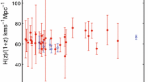
• (iv) We also produce H(z) simulations based on the current cosmic chronometer data, which consists of $N_z=31$ measurements presented in 1 – see also Table I in [27].

Such a prescription provides a benchmark to test the performance of the ML algorithms deployed.

Table 1 31 CC H(z) measurements obtained from the differential age method used in our analysis

2.2 Uncertainty estimation

Although these algorithms are able to provide measurements of $H_0$ at a given redshift, they do not provide their uncertainties. We develop a Monte Carlo-bootstrap (MC-bootstrap) method for this purpose, described as follows

• Rather than creating a single simulation centered on the fiducial model for each data-set (item (i) of Sect. 2), we produce H(z) measurements at a given redshift following a normal distribution centred around its fiducial value according to ${\mathcal {N}}(H^{\textrm{fid}}(z),\sigma _{H}/H)$. $H^{\textrm{fid}}(z)$ represents the H(z) value given by the fiducial Cosmology, whereas $\sigma _{H}$ consists on its uncertainty as described in the item (iii) of Sect. 2.

• As for the “real data” simulations, described in item (iv) of Sect. 2, we replace the ith H(z) measurement presented in the second column of Table 1 by a value drawn from a normal distribution centered on the fiducial model, i.e, ${\mathcal {N}}(H^{\textrm{fid}}(z_i),\sigma _{H;i})$, where $z_i$ represents the redshift of each data point and $\sigma _{H;i}$ its corresponding uncertainty – first and third columns in Table 1, respectively.

• We repeat this procedure 100 times for each data-set of $N_z$ data-points with $\sigma _H/H$ uncertainties as described in the item (iii) and (iv) of Sect. 2.

• The 100 MC realisations produced for each case are provided as inputs for each ML algorithms described in Sect. 3.1.

• We report the average and standard deviation of these 100 values as the $H_0$ measurement and uncertainty, respectively, for each $N_z$ and $\sigma _H/H$ case. Same applies for the “real data” simulations.

3 Analysis

3.1 Methods

Our regression analysis are carried out on all simulated and “real” data-sets with several ML algorithms available in the scikit-learn package¹ [90]. Firstly we divide our input sample into training and testing data-sets as

so that our testing sub-set contains 25% of the original sample size. Then we deploy different ML algorithms on the training test, looking for the “best combination” of hyperparameters with the help of GridSearchCV.² This function of scikit-learn, given a ML method, performs the learning with all the combination of hyperparameters and shows the performance of every combination – or each one of them – during the cross-validation (CV) procedure .³ Such a procedure is performed for the sake of avoiding overfitting on the test set. We chose CV $=3$ in our analysis, given the limited number of H(z) data-points.

The ML methods deployed in our analysis are given as follows:

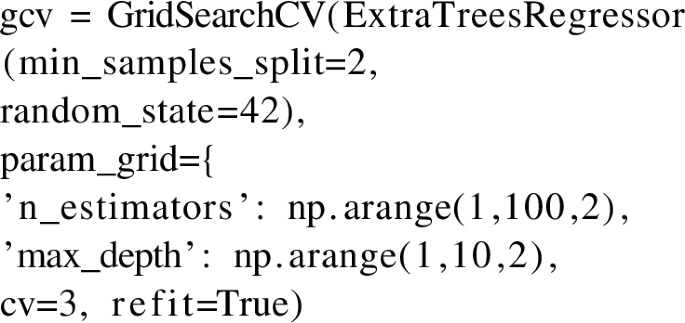
• Extra-Trees (EXT): An ensemble of randomised decision trees (extra-trees). The goal of the algorithm is to create a model that predicts the value of a target variable by learning simple decision rules inferred from the data features. A tree can be seen as a piecewise constant approximation⁴ [91]. We evaluate the algorithm hyperpameter values that best fit the input simulations through a grid search. Hence, our grid search over the EXT hyperpameters are given by:

  

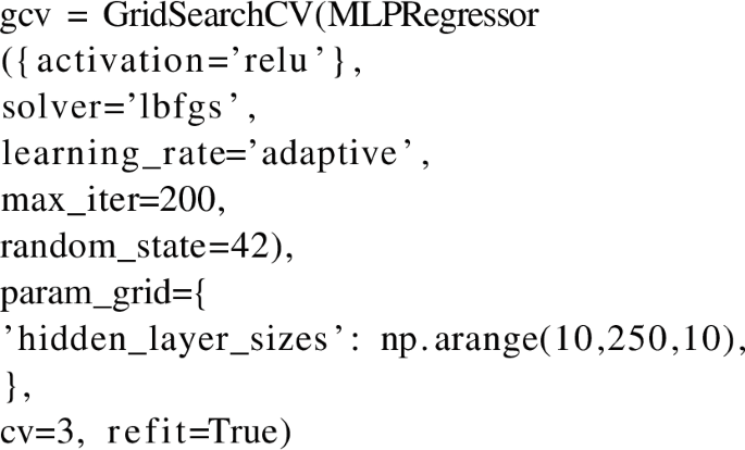
• Artificial Neural Network (ANN): A Multi-layered Perceptron algorithm that trains using backpropagation with no activation function in the output layer⁵ [92]. The ANN hyperparameter grid search consists of:

  

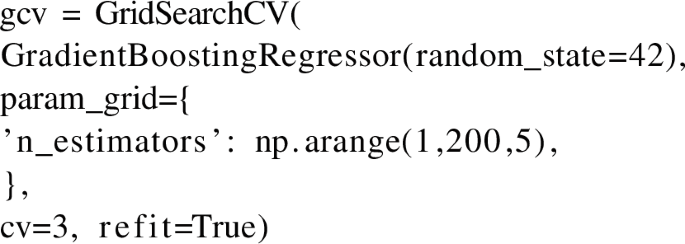
• Gradient Boosting Regression (GBR): This estimator builds an additive model in a forward stage-wise fashion; it allows for the optimisation of arbitrary differentiable loss functions. In each stage a regression tree is fit on the negative gradient of the given loss function⁶ [93]. The grid search over the GBR hyperparameters corresponds to:

  

• Support Vector Machines (SVM): A linear model that creates a line or hyperplane to separate data into different classes [94, 95]. Originally developed for classification problems, it was also extended for regression, as in the goal of this work.⁷ The hyperparameter grid search of the SVM method reads

  

Note that we adopted the default evaluation metric for each ML algorithm as defined by the scikit-learn package. So the EXT method uses the squared error metric to define the quality of the tree split – likewise for the GBR and ANN loss functions - whereas the SVM method assumes $\epsilon =0.1$, so that samples whose prediction is at least $\epsilon$ away from their true target are penalised.⁸

In order to evaluate the performance of these methods, we report the results of the training and test score as

Moreover, we deploy the well-known Gaussian Processes regression (GAP) algorithm on the same simulated data-sets using the GaPP package [81]. We compare the results obtained with the ML algorithms just described with GAP since the latter has been widely used in the literature for similar purposes for about a decade. Two GAP kernels are assumed in our analysis, namely the Squared Exponential (SqExp) and Matérn(5/2) (Mat52). We justify these choices on the basis that the SqExp kernel exhibits greater differentiability than the Mat52, which may result in a larger degree of smoothing on the data reconstruction – hence, smaller reconstruction uncertainties – that may or may not fully represent the underlying data.

3.2 Robustness of results

We define the bias (b) as the average displacement of the predicted Hubble Constant ($H^{\textrm{pred}}_0$), obtained from the MC-bootstrap method, from the fiducial value, i.e., $\Delta H_0=H^{\textrm{pred}}_0 - H^{\textrm{fid}}_0$, and the Mean Squared Error (MSE) as the average squared displacement:

$$\begin{aligned} \textrm{b} = \langle \Delta H_0 \rangle , ~~~ \textrm{MSE} = \langle \Delta H_0^2 \rangle . \end{aligned}$$

(6)

Using the definition of variance, we estimate the bias-variance tradeoff of our analysis

$$\begin{aligned} \textrm{BVT} = \langle \Delta H_0^2 \rangle - \langle \Delta H_0 \rangle ^2 = \textrm{MSE} - \textrm{b}^2 \;, \end{aligned}$$

(7)

therefore we can evaluate the performance of these algorithms for each simulated data-set specification.

4 Results

Fig. 1

$H_0$ measurements from the algorithm EXT (top left), ANN (top right), GBR (center left), SVM (center right), SqExp (lower left) and Mat52 (lower right), plotted against the number of simulated H(z) measurements. Each data point represents different $\sigma _H/H$ values, whereas the light blue horizontal lines denote the fiducial $H_0$ value

Fig. 2

Same as Fig. 1, but for the BVT. Each data point corresponds to different $\sigma _H/H$ values

Fig. 3

The reconstructed H(z) values obtained from EXT (top left), ANN (top right), GBR (center left), SVM (center right), SqExp (lower left) and Mat52 (lower right). Different shades of magenta represent different confidence level for the reconstructions, ranging from 1 (darker shade) to $3\sigma$ (lighter shade)

We show our $H_0$ measurements for each algorithm in Fig. 1. The top panels present the results obtained from the EXT (left) and ANN (right) algorithms, whereas the middle panels display the GBR (left) and SVM (right) results, and the bottom ones show the GAP predictions for the Mat52 and SqExp kernels in the left and right plots, respectively. Each data point at these plots represents the predicted $H_0$ values ($H^{\textrm{pred}}_0$) according to the prescription described in Sect. 2.1 for each simulated data-set specifications, i.e., different $\sigma _{H}/H$ results against the $N_z$ values. The light blue horizontal line corresponds to the fiducial $H_0$. We can see that GBR and EXT are able to correctly predict the fiducial $H_0$ for higher $N_z$ and lower $\sigma _{H}/H$ values, but not otherwise – especially for low values of $N_z$, where these algorithms predict a larger $H_0$ value. This indicates a bias in the results, despite the cross-validation procedure adopted. We also find that ANN and SVM are able to recover the fiducial $H_0$, even for lower quality sets of simulations. However, its predictions present larger variances as $\sigma _{H}/H$ increases.

These results show that GBR and EXT are more sensitive to $N_z$ concerning bias, whereas ANN is more sensitive to $\sigma _{H}/H$ with respect to its variance. On the other hand, SVM exhibits the best bias-variance tradeoff among all algorithms, as shown in Fig. 2, along with Tables 2, 3, 4, 5 and 6, presented in Appendix B. We obtain that SVM is able to recover the fiducial $H_0$ without significant losses in bias and variance as the simulation quality decreases. Such a result may happen due to a few reasons: For example, due to the non-guaranteed convergence of neural networks. By an appropriate choice of hyperparameters, ANN can approach a target function until a satisfactory result is reached; however, SVMs are theoretically grounded in their capacity to converge to the solution for a problem. Note that we adopted a polynomial kernel for SVM, and a nonlinear activaction function for ANN, namely “relu”, in order to make a fair comparison between them. As for the EXT case, such an algorithm is known to be prone to overfitting and to outliers, which can explain the larger bias with lower variance. A similar problem applies for the GBR case as well. Not to mention that both demand a longer training time than ANN and SVM, which translates into a longer computational time to obtain the $H_0$ measurements and uncertainties in our case.

Regarding the comparison with the results obtained with GAP using the Squared Exponential (SqExp) and Matérn(5/2) (Mat52) kernels, we find good agreement between the SVM and GAP measurement of $H_0$, in spite of a slightly larger BVT for the former. But note that GAP can also be prone to overfitting, as the data points with smaller uncertainties have a greater impact to determine the function that best represents the distance between data points to perform its numerical reconstruction – especially when assuming the SqExp kernel, which presents greater differentiability than the Mat52 case. Therefore, we show that SVM can be used as a cross-check method for GAP regression, which has been widely used in the literature..

Moreover, we show the H(z) reconstructions obtained from the simulations mimicking the real data configuration in Fig. 3, at a 1, 2 and $3\sigma$ confidence level, alongside the actual H(z) measurements. We can clearly see a “step-wise” behaviour on the EXT and GBR reconstructions, contrarily to other algorithms. This illustrates the bias problems they face, as commented before. Once again, the GAP results exhibit the smallest uncertainties among all, but this may also happen due to possible overfitting, as commented before. This is exemplified by the dip on the high-z end of the reconstruction. Nevertheless, the Hubble Constant measured by all algorithms are in agreement with each other, as depicted in Table 7, where EXT and GBR again exhibit a tendency towards larger $H_0$ values – and hence larger BVT – while ANN and SVM present less biased results, as in the previous cases. Interestingly, we find that ANN performed slightly better than SVM this time around, yielding a slightly lower BVT. Note also that our results are in good agreement with the predicted $H_0$ in [27], who used ANN as well in their analysis,⁹ but we could obtain a slightly lower uncertainty in our predictions – roughly 17% uncertainty versus 23% in their case.

We also checked whether the test sample size affects the $H_0$ predictions and their bias-variance tradeoff. We find that its default choice, i.e., a split between 75 and 25% between training and test sample, respectively, provides the best results for all algorithms compared to a 90–10% and 60–40% split, for instance. The EXT and GBR algorithms perform similarly for 10% and 25%, but their predictions become significantly worse for the 40% case. This is an expected result, since both algorithms require large training sets to carry out such predictions. On the other hand, ANN and SVM perform significantly worse for split choices other than the default one. Finally, we verified the results for different cross-validations values, such as CV $=2,4,8$, finding consistent values with those obtained with the standard choice CV $=3$.

5 Conclusions

Machine learning has been gaining formidable importance in present times. Given the state-of-art of modern computation and processing facilities, the application of machine learning algorithms in physical sciences not only became popular, but essential in the process of handling huge data-sets and performing model prediction - specially in light of forthcoming redshift surveys.

Our work focused on a comparison of different machine learning algorithms for the sake of measuring the Hubble Constant from cosmic chronometers measurements. We used four different algorithms in our analysis, which are based on decision trees, artificial neural networks, support vector machine and gradient boosting, as available in the scikit-learn python package. We applied them on simulated H(z) data-sets assuming different specifications, and assuming a flat $\Lambda$CDM model consistent with Planck 2018 best fit, in order to measure $H_0$ through an extrapolation procedure.

Our uncertainties are estimated using a Monte Carlo-bootstrap method on the simulations, after properly splitting them into training and test sets, and performed a grid search over their hyperparameter space during the cross-validation procedure. In addition, we created a performance ranking between these methods via the bias-variance tradeoff, and compared them with other established methods in the literature, e.g. Gaussian Processes as in the GaPP code.

We obtained that the algorithms based on decision trees and gradient boosting present the lowest performance among all, as they provide low variance with a large bias in the reconstructed $H_0$. Instead, the artificial neural networks and support vector machine are able to correctly recover the fiducial $H_0$ value, where the latter method exhibits the lowest variance among them. We also found that the support vector machine algorithm presents compatible benchmark metrics with the Gaussian Processes one. This result shows that such method can be successfully used as a cross-check method between different non-parametric reconstruction techniques, which will be of great importance in the advent of next-generation cosmological surveys [14,15,16,17,18,19], as they are expected to provide H(z) measurements with a few percent precision.

Appendix A: Algorithm performance results

See Tables 2, 3, 4, 5, 6 and 7.

Table 2 Respectively: $H_0$ measurements (in units of $\textrm{km s}^{-1} \; \textrm{Mpc}^{-1}$), as well as the BVT values obtained for all $N_z$ and ML algorithms assuming $\sigma _H/H=0.008$. We also show the results obtained using the GAP method at the bottom of the table

Table 3 Same as Table 2, but assuming $\sigma _H/H=0.01$

Table 4 Same as Table 2, but assuming $\sigma _H/H=0.03$

Table 5 Same as Table 2, but assuming $\sigma _H/H=0.05$

Table 6 Same as Table 2, but assuming $\sigma _H/H=0.08$

Table 7 Same as Table 2, but assuming the real data configuration, i.e., $N_z=31$ and the same $\sigma _{H(z)}$ of the real H(z) measurements

References

A.G. Riess et al., [Supernova Search Team], Observational evidence from supernovae for an accelerating universe and a cosmological constant. Astron. J. 116, 1009–1038 (1998). arXiv:astro-ph/9805201
S. Perlmutter et al., [Supernova Cosmology Project], Measurements of \(\Omega \) and \(\Lambda \) from 42 high redshift supernovae. Astrophys. J. 517, 565–586 (1999). arXiv:astro-ph/9812133
N. Aghanim, et al., [Planck Collaboration], Planck 2018 results. VI. Cosmological parameters. Astron. Astrophys. 641, A6 (2020). (Erratum: Astron. Astrophys. 652 (2021), C4) arXiv:1807.06209
D.M. Scolnic, et al., The complete light-curve sample of spectroscopically confirmed SNe Ia from Pan-STARRS1 and cosmological constraints from the combined pantheon sample. Astrophys. J. 859(2), 101 (2018). arXiv:1710.00845
S. Alam, et al. [eBOSS], The Completed SDSS-IV extended Baryon oscillation spectroscopic survey: cosmological implications from two decades of spectroscopic surveys at the apache point observatory. Phys. Rev. D 103(8), 083533 (2021). arXiv:2007.08991
C. Heymans et al., KiDS-1000 cosmology: multi-probe weak gravitational lensing and spectroscopic galaxy clustering constraints. Astron. Astrophys. 646, A140 (2021). arXiv:2007.15632
T.M.C. Abbott, et al., [DES], Dark energy survey year 3 results: cosmological constraints from galaxy clustering and weak lensing. Phys. Rev. D 105(2), 023520 (2022). arXiv:2105.13549
L.F. Secco, et al. [DES], Dark energy survey year 3 results: cosmology from cosmic shear and robustness to modeling uncertainty. Phys. Rev. D 105(2), 023515 (2022). arXiv:2105.13544
S. Weinberg, The cosmological constant problem. Rev. Mod. Phys. 61, 1–23 (1989)
T. Padmanabhan, Cosmological constant: the weight of the vacuum. Phys. Rep. 380, 235–320 (2003). arXiv:hep-th/0212290
E. Di Valentino, O. Mena, S. Pan, L. Visinelli, W. Yang, A. Melchiorri, D.F. Mota, A.G. Riess, J. Silk, In the realm of the Hubble tension—a review of solutions. Class. Quantum Gravity 38(15), 153001 (2021). arXiv:2103.01183
P. Shah, P. Lemos, O. Lahav, A buyer’s guide to the Hubble constant. Astron. Astrophys. Rev. 29(1), 9 (2021). arXiv:2109.01161
A.G. Riess, W. Yuan, L.M. Macri, D. Scolnic, D. Brout, S. Casertano, D.O. Jones, Y. Murakami, L. Breuval, T.G. Brink, et al., A comprehensive measurement of the local value of the hubble constant with 1 km/s/Mpc uncertainty from the hubble space telescope and the SH0ES Team. arXiv:2112.04510
N. Benitez, et al., [J-PAS], J-PAS: The Javalambre-physics of the accelerated universe astrophysical survey. arXiv:1403.5237
S. Bonoli, et al., The miniJPAS survey: a preview of the Universe in 56 colours. Astron. Astrophys. 653, A31 (2021). arXiv:2007.01910
A. Aghamousa, et al., [DESI Collaboration], The DESI experiment part I: science,targeting, and survey design. arXiv:1611.00036
L. Amendola et al., Cosmology and fundamental physics with the Euclid satellite. Living Rev. Relativ. 21, 2 (2018). arXiv:1606.00180
D.J. Bacon et al., [SKA Collaboration], Cosmology with phase 1 of the square kilometre array: red book 2018: technical specifications and performance forecasts. Publ. Astron. Soc. Austral. 37, e007 (2020). arXiv:1811.02743
D. Alonso, et al., [LSST Dark Energy Science], The LSST Dark Energy Science Collaboration (DESC) Science Requirements Document. arXiv:1809.01669
G. Carleo et al., Machine learning and the physical sciences. Rev. Mod. Phys. 91(4), 045002 (2019). arXiv:1903.10563
M. Ntampaka, et al., The role of machine learning in the next decade of cosmology. arXiv:1902.10159
S.Y. Li, Y.L. Li, T.J. Zhang, Model comparison of dark energy models using deep network. Res. Astron. Astrophys. 19, 137 (2019). arXiv:1907.00568
T. Liu, S. Cao, J. Zhang, S. Geng, Y. Liu, X. Ji, Z.H. Zhu, Implications from simulated strong gravitational lensing systems: constraining cosmological parameters using Gaussian Processes. Astrophys. J. 886, 94 (2019). arXiv:1910.02592
Y. Wu, S. Cao, J. Zhang, T. Liu, Y. Liu, S. Geng, Y. Lian, Exploring the “\(L\)–” relation of HII galaxies and giant extragalactic HII regions acting as standard candles. arXiv:1911.10959
R. Arjona, S. Nesseris, What can machine learning tell us about the background expansion of the universe? Phys. Rev. D 101(12), 123525 (2020). arXiv:1910.01529
C. Escamilla-Rivera, M.A.C. Quintero, S. Capozziello, A deep learning approach to cosmological dark energy models. JCAP 03, 008 (2020). arXiv:1910.02788
G.J. Wang, X.J. Ma, S.Y. Li, J.Q. Xia, Reconstructing functions and estimating parameters with artificial neural networks: a test with a hubble parameter and SNe Ia. Astrophys. J. Suppl. 246(1), 13 (2020). arXiv:1910.03636
G.J. Wang, S.Y. Li, J.Q. Xia, ECoPANN: a framework for estimating cosmological parameters using artificial neural networks. Astrophys. J. Suppl. 249(2), 25 (2020). arXiv:2005.07089
Y.C. Wang, Y.B. Xie, T.J. Zhang, H.C. Huang, T. Zhang, K. Liu, Likelihood-free cosmological constraints with artificial neural networks: an application on hubble parameters and SN Ia. Astrophys. J. Suppl. 254(2), 43 (2021). arXiv:2005.10628
T. Liu, S. Cao, S. Zhang, X. Gong, W. Guo, C. Zheng, Revisiting the cosmic distance duality relation with machine learning reconstruction methods: the combination of HII galaxies and ultra-compact radio quasars. Eur. Phys. J. C 81(10), 903 (2021). arXiv:2110.00927
C. García, C. Santa, A.E. Romano, Deep learning reconstruction of the large scale structure of he Universe from luminosity distance observations. Mon. Not. R. Astron. Soc. 518(2), 2241–2246 (2022). arXiv:2107.05771
K. Dialektopoulos, J.L. Said, J. Mifsud, J. Sultana, K.Z. Adami, Neural network reconstruction of late-time cosmology and null tests. JCAP 02(02), 023 (2022). arXiv:2111.11462
P. Mukherjee, J.L. Said, J. Mifsud, Neural network reconstruction of \(H^{\prime }(z)\) and its application in teleparallel gravity. JCAP 12, 029 (2022). arXiv:2209.01113
I. Gómez-Vargas, R.M. Esquivel, R. García-Salcedo, J.A. Vázquez, Neural network reconstructions for the Hubble parameter, growth rate and distance modulus. Eur. Phys. J. C 83(4), 304 (2023). arXiv:2104.00595
L. Tonghua, C. Shuo, M. Shuai, L. Yuting, Z. Chenfa, W. Jieci, What are recent observations telling us in light of improved tests of distance duality relation? Phys. Lett. B 838, 137687 (2023). arXiv:2301.02997
S. Agarwal, F.B. Abdalla, H.A. Feldman, O. Lahav, S.A. Thomas, PkANN-I. Non-linear matter power spectrum interpolation through artificial neural networks. Mon. Not. R. Astron. Soc. 424, 1409–1418 (2012). arXiv:1203.1695
S. Agarwal, F.B. Abdalla, H.A. Feldman, O. Lahav, S.A. Thomas, pkann-II. A non-linear matter power spectrum interpolator developed using artificial neural networks. Mon. Not. R. Astron. Soc. 439(2), 2102–2121 (2014). arXiv:1312.2101
S. Ravanbakhsh, J. Oliva, S. Fromenteau, L.C. Price, S. Ho, J. Schneider, B. Poczos, Estimating cosmological parameters from the dark matter distribution. arXiv:1711.02033
J. Merten, C. Giocoli, M. Baldi, M. Meneghetti, A. Peel, F. Lalande, J.L. Starck, V. Pettorino, On the dissection of degenerate cosmologies with machine learning. Mon. Not. R. Astron. Soc. 487(1), 104–122 (2019). arXiv:1810.11027
A. Peel, F. Lalande, J.L. Starck, V. Pettorino, J. Merten, C. Giocoli, M. Meneghetti, M. Baldi, Distinguishing standard and modified gravity cosmologies with machine learning. Phys. Rev. D 100(2), 023508 (2019). arXiv:1810.11030
D. Ribli, B.Á. Pataki, J.M.Z. Matilla, D. Hsu, Z. Haiman, I. Csabai, Weak lensing cosmology with convolutional neural networks on noisy data. Mon. Not. R. Astron. Soc. 490(2), 1843–1860 (2019). arXiv:1902.03663
J. Fluri, T. Kacprzak, A. Lucchi, A. Refregier, A. Amara, T. Hofmann, A. Schneider, Cosmological constraints with deep learning from KiDS-450 weak lensing maps. Phys. Rev. D 100(6), 063514 (2019). arXiv:1906.03156
S. Pan, M. Liu, J. Forero-Romero, C.G. Sabiu, Z. Li, H. Miao, X.D. Li, Cosmological parameter estimation from large-scale structure deep learning. Sci. China Phys. Mech. Astron. 63(11), 110412 (2020). arXiv:1908.10590
M. Ntampaka, D.J. Eisenstein, S. Yuan, L.H. Garrison, A hybrid deep learning approach to cosmological constraints from galaxy redshift surveys. arXiv:1909.10527
J.M.Z. Matilla, M. Sharma, D. Hsu, Z. Haiman, Interpreting deep learning models for weak lensing. Phys. Rev. D 102(12), 123506 (2020). arXiv:2007.06529
F. Villaescusa-Navarro, S. Genel, D. Angles-Alcazar, L. Thiele, R. Dave, D. Narayanan, A. Nicola, Y. Li, P. Villanueva-Domingo, B. Wandelt, et al., The CAMELS multifield data set: learning the universe’s fundamental parameters with artificial intelligence. Astrophys. J. Suppl. 259(2), 61 (2022). arXiv:2109.10915
H.M. Kamdar, M.J. Turk, R.J. Brunner, Machine learning and cosmological simulations-I. Semi-analytical models. Mon. Not. R. Astron. Soc. 455(1), 642–658 (2016). arXiv:1510.06402
H.M. Kamdar, M.J. Turk, R.J. Brunner, Machine learning and cosmological simulations-II. Hydrodynamical simulations. Mon. Not. R. Astron. Soc. 457(2), 1162–1179 (2016). arXiv:1510.07659
L. Lucie-Smith, H.V. Peiris, A. Pontzen, M. Lochner, Machine learning cosmological structure formation. Mon. Not. R. Astron. Soc. 479(3), 3405–3414 (2018). arXiv:1802.04271
S. He, Y. Li, Y. Feng, S. Ho, S. Ravanbakhsh, W. Chen, B. Póczos, Learning to predict the cosmological structure formation. Proc. Nat. Acad. Sci. 116(28), 13825–13832 (2019). arXiv:1811.06533
D.K. Ramanah, T. Charnock, G. Lavaux, Painting halos from cosmic density fields of dark matter with physically motivated neural networks. Phys. Rev. D 100(4), 043515 (2019). arXiv:1903.10524
L. Lucie-Smith, H.V. Peiris, A. Pontzen, An interpretable machine learning framework for dark matter halo formation. Mon. Not. R. Astron. Soc. 490(1), 331–342 (2019). arXiv:1906.06339
M. Tsizh, B. Novosyadlyj, Y. Holovatch, N.I. Libeskind, Large-scale structures in the \(\Lambda \)CDM Universe: network analysis and machine learning. Mon. Not. R. Astron. Soc. 495(1), 1311–1320 (2020). arXiv:1910.07868
K. Murakami, A.J. Nishizawa, Identifying cosmological information in a deep neural network. arXiv:2012.03778
J. Chacón, J.A. Vázquez, E. Almaraz, Classification algorithms applied to structure formation simulations. Astron. Comput. 38, 100527 (2022). arXiv:2106.06587
R. von Marttens, L. Casarini, N.R. Napolitano, S. Wu, V. Amaro, R. Li, C. Tortora, A. Canabarro, Y. Wang, Inferring galaxy dark halo properties from visible matter with machine learning. Mon. Not. R. Astron. Soc. arXiv:2111.01185
D. Piras, B. Joachimi, F. Villaescusa-Navarro, Fast and realistic large-scale structure from machine-learning-augmented random field simulations. arXiv:2205.07898
S. Hassan, A. Liu, S. Kohn, P. La Plante, Identifying reionization sources from 21 cm maps using convolutional neural networks. Mon. Not. R. Astron. Soc. 483(2), 2524–2537 (2019). arXiv:1807.03317
N. Gillet, A. Mesinger, B. Greig, A. Liu, G. Ucci, Deep learning from 21-cm tomography of the cosmic dawn and reionization. Mon. Not. R. Astron. Soc. 484(1), 282–293 (2019). arXiv:1805.02699
J. Chardin, G. Uhlrich, D. Aubert, N. Deparis, N. Gillet, P. Ocvirk, J. Lewis, A deep learning model to emulate simulations of cosmic reionization. Mon. Not. R. Astron. Soc. 490(1), 1055–1065 (2019). arXiv:1905.06958
P. La Plante, M. Ntampaka, Machine learning applied to the reionization history of the universe in the 21 cm signal. Astrophys. J. 810, 110 (2019). arXiv:1810.08211
T. Mangena, S. Hassan, M.G. Santos, Constraining the reionization history using deep learning from 21 cm tomography with the square kilometre array. Mon. Not. R. Astron. Soc. 494(1), 600–606 (2020). arXiv:2003.04905
S. Hassan, S. Andrianomena, C. Doughty, Constraining the astrophysics and cosmology from 21 cm tomography using deep learning with the SKA. Mon. Not. R. Astron. Soc. 494(4), 5761–5774 (2020). arXiv:1907.07787
D. Prelogović, A. Mesinger, S. Murray, G. Fiameni, N. Gillet, Machine learning astrophysics from 21 cm lightcones: impact of network architectures and signal contamination. Mon. Not. R. Astron. Soc. 509(3), 3852–3867 (2021). arXiv:2107.00018
A.A. Collister, O. Lahav, ANNz: estimating photometric redshifts using artificial neural networks. Publ. Astron. Soc. Pac. 116, 345–351 (2004). arXiv:astro-ph/0311058
R. Hogan, M. Fairbairn, N. Seeburn, GAz: a genetic algorithm for photometric redshift estimation. Mon. Not. R. Astron. Soc. 449(2), 2040–2046 (2015). arXiv:1412.5997
I. Sadeh, F.B. Abdalla, O. Lahav, ANNz2-photometric redshift and probability distribution function estimation using machine learning. Publ. Astron. Soc. Pac. 128(968), 104502 (2016). arXiv:1507.00490
M. Bilicki, et al., Photometric redshifts for the kilo-degree survey. Machine-learning analysis with artificial neural networks. Astron. Astrophys. 616, A69 (2018). arXiv:1709.04205
Z. Gomes, M.J. Jarvis, I.A. Almosallam, S.J. Roberts, Improving photometric redshift estimation using GPz: size information, post processing and improved photometry. Mon. Not. R. Astron. Soc. 475(1), 331–342 (2018). arXiv:1712.02256
G. Desprez, et al., [Euclid], Euclid preparation: X. The \(Euclid\) photometric-redshift challenge. Astron. Astrophys. 644, A31 (2020). arXiv:2009.12112
L. Cabayol, M. Eriksen, A. Amara, J. Carretero, R. Casas, F.J. Castander, J. De Vicente, E. Fernández, J. García-Bellido, E. Gaztanaga, et al., The PAU survey: estimating galaxy photometry with deep learning. Mon. Not. R. Astron. Soc. 506(3), 4048–4069 (2021). arXiv:2104.02778
S. Kunsági-Máté, R. Beck, I. Szapudi, I. Csabai, Photometric redshifts for quasars from WISE-PS1-STRM. (2022). arXiv:2206.01440
A. Kurcz, M. Bilicki, A. Solarz, M. Krupa, A. Pollo, K. Małek, Towards automatic classification of all WISE sources. Astron. Astrophys. 592, A25 (2016). arXiv:1604.04229
E.J. Kim, R.J. Brunner, Star-galaxy classification using deep convolutional neural networks. Mon. Not. R. Astron. Soc. 464(4), 4463–4475 (2017). arXiv:1608.04369
R. Beck, I. Szapudi, H. Flewelling, C. Holmberg, E. Magnier, PS1-STRM: neural network source classification and photometric redshift catalogue for PS1 \(3\pi \) DR1. Mon. Not. R. Astron. Soc. 500(2), 1633–1644 (2020). arXiv:1910.10167
P.O. Baqui, et al., The miniJPAS survey: star-galaxy classification using machine learning. Astron. Astrophys. 645, A87 (2021). arXiv:2007.07622
M. Lochner, J.D. McEwen, H.V. Peiris, O. Lahav, M.K. Winter, Photometric supernova classification with machine learning. Astrophys. J. Suppl. 225(2), 31 (2016). arXiv:1603.00882
D. Muthukrishna, D. Parkinson, B. Tucker, DASH: deep learning for the automated spectral classification of supernovae and their hosts. Astrophys. J. 885, 85 (2019). arXiv:1903.02557
D. Muthukrishna, G. Narayan, K.S. Mandel, R. Biswas, R. Hložek, RAPID: early classification of explosive transients using deep learning. Publ. Astron. Soc. Pac. 131(1005), 118002 (2019). arXiv:1904.00014
C. Fremling, X.J. Hall, M.W. Coughlin, A.S. Dahiwale, D.A. Duev, M.J. Graham, M.M. Kasliwal, E.C. Kool, A.A. Mahabal, A.A. Miller, et al., SNIascore: deep-learning classification of low-resolution supernova spectra. Astrophys. J. Lett. 917(1), L2 (2021). arXiv:2104.12980
M. Seikel, C. Clarkson, M. Smith, Reconstruction of dark energy and expansion dynamics using Gaussian processes. JCAP 06, 036 (2012). arXiv:1204.2832. GaPP is available at https://github.com/astrobengaly/GaPP
R. Jimenez, L. Verde, T. Treu, D. Stern, Constraints on the equation of state of dark energy and the Hubble constant from stellar ages and the CMB. Astrophys. J. 593, 622–629 (2003). arXiv:astro-ph/0302560
J. Simon, L. Verde, R. Jimenez, Constraints on the redshift dependence of the dark energy potential. Phys. Rev. D 71, 123001 (2005). arXiv:astro-ph/0412269
D. Stern, R. Jimenez, L. Verde, M. Kamionkowski, S.A. Stanford, Cosmic chronometers: constraining the equation of state of dark energy. I: H(z) Measurements. JCAP 02, 008 (2010). arXiv:0907.3149
M. Moresco, A. Cimatti, R. Jimenez, L. Pozzetti, G. Zamorani, M. Bolzonella, J. Dunlop, F. Lamareille, M. Mignoli, H. Pearce, et al., Improved constraints on the expansion rate of the Universe up to z 1.1 from the spectroscopic evolution of cosmic chronometers. JCAP 08, 006 (2012). arXiv:1201.3609
C. Zhang, H. Zhang, S. Yuan, S. Liu, T.-J. Zhang, Y.-C. Sun, Four new observational \(H(z)\) data from luminous red galaxies of Sloan digital sky survey data release seven. Res. Astron. Astrophys. 14, 1221–1233 (2014). arXiv:1207.4541
M. Moresco, Raising the bar: new constraints on the Hubble parameter with cosmic chronometers at z \(\sim \) 2. Mon. Not. R. Astron. Soc. 450(1), L16–L20 (2015). arXiv:1503.01116
M. Moresco, L. Pozzetti, A. Cimatti, R. Jimenez, C. Maraston, L. Verde, D. Thomas, A. Citro, R. Tojeiro, D. Wilkinson, A 6% measurement of the Hubble parameter at \(z\sim 0.45\): direct evidence of the epoch of cosmic re-acceleration. JCAP 05, 014 (2016). arXiv:1601.01701
A.L. Ratsimbazafy, S.I. Loubser, S.M. Crawford, C.M. Cress, B.A. Bassett, R.C. Nichol, P. Väisänen, Age-dating luminous red galaxies observed with the Southern African large telescope. Mon. Not. R. Astron. Soc. 467(3), 3239–3254 (2017). arXiv:1702.00418
F. Pedregosa et al., Scikit-learn: machine learning in Python. J. Mach. Learn. Res. 12, 2825 (2011). https://scikit-learn.org/stable/index.html
L. Breiman, J. Friedman, R. Olshen, C. Stone, Classification and Regression Trees (Wadsworth, Belmont, 1984)
D.E. Rumelhart, G.E. Hinton, R.J. Williams, Learning representations by back-propagating errors. Nature 323, 533 (1986)
J.H. Friedman, Greedy function approximation: a gradient boosting machine. Ann. Stat. 29, 1189
C.M. Bishop, Pattern Recognition and Machine Learning (Springer, Berlin, 2006)
A.J. Smola, B. Schölkopf, A tutorial on support vector regression. Stat. Comput. 14, 199 (2004)
Acknowledgements
We thank the annonymous referee for constructive criticism on the manuscript. CB acknowledges financial support from the FAPERJ postdoc nota 10 fellowship. LC acknowledges financial support from CNPq (Grant No. 310314/2019-4). J. Alcaniz is supported by Conselho Nacional de Desenvolvimento Científico e Tecnológico CNPq (Grants no. 310790/2014-0 and 400471/2014-0) and Fundação de Amparo à Pesquisa do Estado do Rio de Janeiro FAPERJ (grant no. 233906). We thank the National Observatory Data Center (CPDON) for computational support.
Author information
Authors and Affiliations
Corresponding author