Shining light into the Higgs portal with $\gamma \gamma$ colliders

Abstract

High-energy $\gamma \gamma$ colliders constitute a potential running mode of future lepton colliders such as the ILC and CLIC. We study the sensitivity of a high-energy $\gamma \gamma$ collider to the Higgs portal scenario to a hidden sector above the invisible Higgs decay threshold. We show that such $\gamma \gamma$ collisions could allow to probe the existence of dark sectors through the Higgs portal with precision competitive with other planned collider facilities, profiting from the unique combination of sizable cross-section with clean final state and collider environment. In addition, this search could cover the singlet Higgs portal parameter space yielding a first-order electroweak phase transition in the early Universe.

1 Introduction

The existence of dark sectors in Nature, uncharged under the gauge symmetries of the Standard Model (SM), and interacting with the SM through the Higgs boson h is a well-motivated possibility: both theoretically, since the operator $H^{\dagger }H$ is the only super-renormalizable SM Lorentz invariant operator singlet under the SM gauge symmetries [1], and in connection to open problems in particle physics and cosmology, like the nature of dark matter (DM) [2,3,4,5]. In addition, a singlet scalar field S coupled to the SM via the Higgs portal Lagrangian interaction $\left| H\right| ^2 S^2$ (with H the SM Higgs doublet) is arguably the simplest possible extension of the SM, further motivated by the fact that it could yield a strongly first-order electroweak (EW) phase transition in the early Universe [6,7,8,9], possibly allowing for EW baryogenesis as the origin of the observed matter-antimatter asymmetry of the Universe [10, 11] (see [12] for a review).

Despite its simplicity and appeal, such a singlet Higgs portal scenario to a dark sector may be challenging to probe experimentally: While strong direct detection DM constraints on this scenario apply if S is the DM particle [13], these constraints are relaxed when considering more fields in the dark sector [14]. In addition, S may belong to the dark sector but not necessarily be itself the DM particle, such that astrophysical/cosmological DM constraints do not directly restrict its properties. The singlet Higgs portal scenario is also very challenging to probe at high-energy colliders in the case that the singlet scalar field S is heavier than $\sim 65$ GeV and the Higgs boson decay $h \rightarrow S S$ is not kinematically open. At the Large Hadron Collider (LHC) it is possible to directly probe the hidden sector above the Higgs decay threshold (i.e. for singlet scalar masses $m_S$ above $m_h/2$) in final states with hadronic jets and missing transverse energy , via the vector-boson-fusion (VBF) process $p p \rightarrow j j\, + S S$ [8, 15] mediated by an off-shell Higgs (see Fig. 1, left), with the pair of singlet scalars giving rise to . The high-luminosity LHC would however only be sensitive to very large values of the Higgs portal coupling [8, 15]. A future FCC-hh [16] hadron collider operating at a center-of-mass energy $\sqrt{s} =$ 100 TeV would improve on the LHC sensitivity [15, 17], profiting from the large enhancement of the VBF off-shell Higgs process at high energy. Yet, the hadronic environment makes it challenging to achieve strong sensitivity improvements. Future high-energy $e^+ e^-$ colliders like the $\sqrt{s} = 1$ TeV International Lineal Collider (ILC) [18,19,20] or the $\sqrt{s} = 1.5/3$ TeV Compact Linear Collider (CLIC) [21] could provide the ideal setup to probe the Higgs portal above the $m_h/2$ threshold, from a combination of reach in energy and clean collision environment. The cross section for the associated production of an off-shell Higgs with a Z boson, $e^+ e^- \rightarrow h^* Z$, is however very small for high center-of-mass energy, whereas for lower center-of-mass energies ($\sqrt{s} \sim 250$ GeV) the cross section for $e^+ e^- \rightarrow h^* Z$ is sizable, but in this case the kinematic reach to the Higgs portal above the $m_h/2$ threshold is very limited [22, 23].¹ In contrast, the VBF off-shell Higgs production becomes important at high energies, yet for $e^+ e^-$ collisions the dominant (W-boson mediated) VBF process producing a pair of singlet scalars via an off-shell Higgs is $e^+ e^- \rightarrow \nu \nu S S$, completely invisible and impossible to trigger on. Subdominant Z-boson mediated VBF processes yield an final state which could be used to probe the Higgs portal [24, 25] (see also [26]), yet at the expense of a significantly smaller cross section. Invisible final states can also be investigated at lepton colliders via single photon + processes (see e.g. [23, 27,28,29]), yet for the case of the Higgs portal scenario, since the mediator to the dark sector is the Higgs particle, the corresponding mono-photon rate is generally proportional to the lepton Yukawas,² and thus very small.

Fig. 1

Feynman diagrams for singlet scalar S pair production through the Higgs portal. Left: hadron colliders (for $e^+ e^-$ colliders, initial state fermions would be $e^{\pm }$, and final state fermions would be neutrinos). Right: $\gamma \gamma$ colliders

In this work, we show that a $\gamma \gamma$ (or $\ell ^{\pm } \gamma$) operating mode of a high-energy lepton collider like ILC or CLIC could overcome the above problems and provide an optimal setup to probe the Higgs portal to a dark sector, via the process , see Fig. 1, right. After discussing the relevant aspects of $\gamma \gamma$ colliders for our analysis in Sect. 2, we introduce the singlet scalar extension of the SM in Sect. 3 as the benchmark scenario for our study (yet, we emphasize that our results apply for any Higgs portal to a dark sector scenario), and briefly discuss its impact on the EW phase transition. We then analyze the sensitivity of an ILC and CLIC-based $\gamma \gamma$ collider to the Higgs portal above threshold scenario in Sect. 4. Finally, we conclude in Sect. 5.

2 Basics of $\gamma \gamma$ colliders

The possibility of a high-energy $\gamma \gamma$ (or $\gamma e$) collider based on a linear $e^{+}e^{-}$ collider has been considered since the early 1980’s [30,31,32]. The physical principle is the generation of high-energy photons through Compton back-scattering of laser photons by the high-energy electrons or positrons of the $e^{+}e^{-}$ collider beams, a mechanism that has subsequently been extensively studied (see e.g. [33,34,35,36,37,38,39,40,41,42]). Here we briefly discuss the aspects of $\gamma \gamma$ colliders relevant to our phenomenological study, and stress that details of these aspects can depend on specifics of the photon collider implementation (see e.g. the discussion in [42]).

In the conversion region a photon with energy $E_{0}$ is scattered on an electron with energy $E_{e}$ at a small collision angle $\alpha$ (almost head-on). The photons from Compton back-scattering have a spectrum with maximum energy $E^{\mathrm {max}}_{\gamma }$ given by

$$\begin{aligned} E^{\mathrm {max}}_{\gamma } =\frac{\kappa }{1+\kappa }E_{e}, \quad \kappa =\frac{4\,E_{e}\,E_{0}\cos ^{2}\left( \alpha /2\right) }{m_{e}^{2}} \end{aligned}$$

(2.1)

where $m_e$ is the electron mass. According to Eq. (2.1), the largest possible laser frequency $\omega _0 = E_0/\hbar$ should be used in order to increase $E^{\mathrm {max}}_{\gamma }$. This also increases the fraction of hard photons in the spectrum [33]. However, at large $\kappa$ the resulting high-energy photons are then converted to $e^{+}e^{-}$ pairs in collisions with laser photons, so the optimum value $\kappa = \kappa ^{\mathrm {max}}$ is the threshold of this conversion process, given for a head-on collision by [33, 41] $E^{\mathrm {max}}_{\gamma } E_{0} = m_e^2$. Combining this threshold condition with Eq. (2.1) yields $\kappa ^{\mathrm {max}}=2\, (1+\sqrt{2}) \approx 4.83$, resulting in a highest energy $E_{\gamma }^{\mathrm {max}} \approx 0.83 E_{e}$.

The energy spectrum of the resulting photon beam is peaked at $E_{\gamma }^{\mathrm {max}}$, and the number of high energy photons dramatically increases for polarised beams with $2\lambda _{e}P_{\gamma }=-1$, being $\lambda _{e}$ ($|\lambda _{e}| \le 1/2$) the mean helicity of the initial electron and $P_{\gamma }$ that of the laser photon. In addition to this high-energy peak there is also a factor 5–8 larger (in luminosity) low-energy spectrum which is produced by multiple Compton scattering and beamstrahlung photons. These low-energy collisions have a large longitudinal boost in the detector reference frame. The $\gamma \gamma$ luminosity ${{\mathcal {L}}}_{\gamma \gamma }$ in the high-energy part of the spectrum is proportional to the geometric luminosity of the electron beams ${{\mathcal {L}}}_{G}$ [35, 39]. Considering $y = E_{\gamma \gamma }/(2E_{e})$, one approximately has [34, 35]

$$\begin{aligned} {{\mathcal {L}}}_{\gamma \gamma }\left( y \,> 0.8 \,y^{\mathrm{max}}\right) \approx 0.1\, {{\mathcal {L}}}_G \, , \end{aligned}$$

(2.2)

where the maximum possible value of y is given by $y^{\mathrm{max}} = E_{\gamma }^{\mathrm {max}}/E_{e} \simeq 0.83$. As discussed in [34, 38, 40], luminosities ${{\mathcal {L}}}_{\gamma \gamma } \left( y \,> 0.8 \,y^{\mathrm{max}}\right) \sim 10^{34}$ cm$^{-2}$ s$^{-1}$ (and perhaps up to $10^{35}$ cm$^{-2}$ s$^{-1}$ [34]) could be reached at a multi-TeV $\gamma \gamma$ collider, comparable to those of the HL-LHC.

Fig. 2

Luminosity spectra ${{\mathcal {L}}}_{\gamma \gamma }(y)$ used in this work: idealized spectrum $\propto \delta (y - y^{\mathrm{max}})$ (black); analytic spectrum ${{\mathcal {L}}}_{\gamma \gamma }^{nc} \left( y\right)$ for $\kappa ^{\mathrm {max}} = 4.8$ and $2\lambda _{e}P_{\gamma }=-1$ (red); spectrum ${{\mathcal {L}}}_{\gamma \gamma }^{c} \left( y\right)$ including multiple Compton scattering effects and beamstrahlung (blue). All of then are normalized to the same value of ${{\mathcal {L}}}_{\gamma \gamma }\left( y \,> 0.8 \,y^{\mathrm{max}}\right)$ (see text for details)

In the rest of this work we consider three different ${{\mathcal {L}}}_{\gamma \gamma }\left( y\right)$ spectra for a multi-TeV $\gamma \gamma$ collider: (i) An perfect (idealized) spectrum, with the energy of the back-scattered photons essentially localized at $E_{\gamma }^{\mathrm {max}} = 0.83 E_{e}$, i.e. ${{\mathcal {L}}}_{\gamma \gamma }\left( y\right) \propto \delta (y - y^{\mathrm{max}})$. (ii) An analytic high-energy $\gamma \gamma$ collider luminosity spectrum for $\kappa ^{\mathrm {max}} = 4.8$ and $2\lambda _{e}P_{\gamma }=-1$ without multiple Compton scattering and beamstrahlung effects obtained from [39] and labelled here ${{\mathcal {L}}}_{\gamma \gamma }^{nc} \left( y\right)$. (iii): A $\sqrt{s} = 3$ TeV luminosity spectrum including the effect at low energies from multiple Compton scatterings and beamstrahlung fitted from [38], labelled here ${{\mathcal {L}}}_{\gamma \gamma }^{c} \left( y\right)$. The rationale for using these three different spectra in our analysis is that the ${{\mathcal {L}}}_{\gamma \gamma }^{nc} \left( y\right)$ and ${{\mathcal {L}}}_{\gamma \gamma }^{c} \left( y\right)$ spectra incorporate varios features w.r.t. the idealized spectrum that will be present in a realistic $\gamma \gamma$ collision environment: the idealized spectrum is unrealistic, yet it yields information on the effect that approximate monochromaticity of the photon spectrum would have (and provides an upper bound on the sensitivity of $\gamma \gamma$ colliders to the Higgs portal); then, ${{\mathcal {L}}}_{\gamma \gamma }^{nc} \left( y\right)$ and ${{\mathcal {L}}}_{\gamma \gamma }^{c} \left( y\right)$ allow us to gauge the impact of multiple Compton scatterings and beamstrahlung, which produce a low-energy tail in the photon spectrum, as a degrading effect on the sensitivity of $\gamma \gamma$ colliders to dark sectors via the Higgs portal. The three spectra are shown jointly in Fig. 2. From these luminosity spectra we can infer the respective photon energy distributions f(x) for the colliding $\gamma$-beams. The relation between the photon energy distribution and the luminosity spectrum of the photon-photon collisions is given by

$$\begin{aligned} {{\mathcal {L}}}_{\gamma \gamma }\left( y\right) = \int _{0}^{x^{\mathrm {max}}} dx_1 \int _{0}^{x^{\mathrm {max}}} dx_2 \, f(x_1) \,f(x_2) \,\, \delta (y - \sqrt{x_1x_2})\nonumber \\ \end{aligned}$$

(2.3)

with $x^{\mathrm{max}} = y^{\mathrm{max}}$. Our de-convolution to obtain f(x) (we note that $f(x_1) = f(x_2)$ for $x_1 = x_2$ since the two colliding $\gamma$-beams are identical) from ${{\mathcal {L}}}_{\gamma \gamma }\left( y\right)$ uses an ansatz for the function f, detailed in Appendix A. The respective photon energy distributions are shown in Fig. 3. The luminosity spectra and associated photon energy distributions will then be used together with a Monte Carlo event generation from MadGraph 5 [43] to construct event samples (which are then checked independently using Whizard [44, 45]) for the SM background and our BSM signal in Sect. 4.

Fig. 3

Photon energy distribution f(x) for the luminosity spectra ${{\mathcal {L}}}_{\gamma \gamma }(y)$ from Fig. 2

3 The singlet scalar extension of the SM

In order to study the phenomenology of the Higgs portal to a dark sector, we consider here its simplest realization, which consists of an extension of the SM by a real scalar singlet field S [3, 4, 6, 10] which is odd under a ${{\mathbb {Z}}}_{2}$ symmetry. The tree-level scalar potential for the theory is

$$\begin{aligned} V_0\left( H,S\right)= & {} -\mu _{H}^{2}|H|^{2} + \lambda _{H} |H|^{4} + \frac{\mu _{S}^{2}}{2}\,S^{2} +\frac{\lambda _{S}}{4}S^{4} \nonumber \\&+ \lambda _{HS}\,|H|^{2}S^{2}\,, \end{aligned}$$

(3.1)

with $H = (0, (v+ h)/\sqrt{2})$ and $v=246$ GeV the EW scale. Boundedness from below of the scalar potential requires $\lambda _{H},\,\lambda _{S} > 0$, $\lambda _{HS} > - \sqrt{\lambda _{H}\lambda _{S}}$, and the size of the singlet couplings $\lambda _{S}$ and $\lambda _{HS}$ is also restricted by perturbative unitarity constraints (the SM Higgs quartic coupling $\lambda _H = m_h^2/(2\,v^2)$ trivially satisfies these constraints), e.g. the perturbative unitarity bound for $\lambda _{S}$ is $\lambda _S < 8\pi /3$ (see e.g. [9]). In this work we consider the singlet couplings in the range $\lambda _S,\,\lambda _{HS} \in [0,\, 2\pi ]$, the upper bound being dictated by perturbativity. These satisfy the various perturbative unitarity and boundedness from below constraints. After EW symmetry breaking, the ${{\mathbb {Z}}}_{2}$ symmetry is preserved for $m_S^2 = \mu _{S}^{2} + \lambda _{HS} \, v^2 > 0$. In this case, the singlet scalar does not mix with the SM Higgs boson after EW symmetry breaking and only interacts with the SM through its portal coupling $\lambda _{HS}$ to the Higgs boson. In particular, if $m_S > m_h/2 \simeq 63$ GeV, the $h \rightarrow S S$ Higgs boson decay into two singlet scalars is forbidden and the only way to access the hidden sector directly (to produce S) is via an off-shell Higgs [8, 15], which makes this scenario very challenging to probe at colliders.

As outlined in the introduction, extending the SM by the singlet scalar field S can have an important impact on the dynamics of EW symmetry breaking in the early Universe. In the SM, this symmetry breaking process – the EW phase transition – is found to be a smooth cross-over using non-perturbative methods [46, 47]. It would then not induce the needed departure from thermal equilibrium to generate the observed matter-antimatter asymmetry at the EW scale. The presence of the singlet field S may dramatically change this conclusion, triggering a first-order EW phase transition strong enough to allow for baryogenesis [6,7,8, 10] or to produce a stochastic background of gravitational waves observable by LISA (see [48, 49] and references therein). The 1-loop (ring-improved) finite-temperature effective potential for the Higgs and singlet fields is given by (we follow [8, 9])

$$\begin{aligned} V\left( h,S\right)= & {} V_0\left( h,S\right) + V_{\mathrm{CW}}\left( h,S\right) \nonumber \\&+ V_{T}\left( h,S,T\right) + V_{r}\left( h,S,T\right) \,, \end{aligned}$$

(3.2)

with $V_0$ the tree-level potential, $V_{\mathrm{CW}}$ the zero-temperature 1-loop Coleman–Weinberg potential, $V_T$ the 1-loop finite-temperature potential and $V_r$ the contribution from the resummation of higher-loop ring diagrams (see [50] for details). In the on-shell renormalization scheme, the Coleman–Weinberg potential reads

$$\begin{aligned} V_{\mathrm{CW}}\left( h,S\right)= & {} \sum _a \frac{(-1)^{s_a} n_a}{64\, \pi ^2} \left[ m_a^4(h,S) \left( \mathrm{log}\frac{m_a^2(h,S)}{m_a^2(v,0)} - \frac{3}{2} \right) \right. \nonumber \\&\left. + 2\, m_a^2(h,S)\,m_a^2(v,0) \right] \,, \end{aligned}$$

(3.3)

with the renormalization conditions $\left. dV_{\mathrm{CW}}/dh\right| _{(v,0)} = 0$ and $\left. d^2V_{\mathrm{CW}}/dh^2\right| _{(v,0)} = 0$, which ensure that the 1-loop zero-temperature Higgs mass and vev are equal to their tree-level values. The number of degrees of freedom for the species $a = (t,\,W,\,Z,\,h,\,G,\,S)$ contributing to the sum in (3.3) are $n_a = (12,\,6,\,3,\,1,\,3,\,1)$, and $s_a = 0 \, (1)$ for bosons (fermions). The field-dependent squared-masses $m_a^2(h,S)$ for the top quark, W and Z bosons, Higgs boson, Goldstone bosons³ (we use the Landau gauge) and singlet scalar are

$$\begin{aligned} m_t^2(h)= & {} \frac{y_t^2}{2} h^2 , \quad \quad m_h^2(h,S) = -\mu _{H}^{2} + 3 \lambda _H h^2 + \lambda _{HS} S^2 \,, \nonumber \\ m_W^2(h)= & {} \frac{g^2}{4} h^2 , \quad \quad m_G^2(h,S) = -\mu _{H}^{2} + \lambda _H h^2 + \lambda _{HS} S^2 \,, \nonumber \\ m_Z^2(h)= & {} \frac{g^2+g'^2}{4} h^2 , \quad \quad m_S^2(h,S) = \mu _{S}^{2} + \lambda _{HS} h^2 + 3 \lambda _S S^2\, . \nonumber \\ \end{aligned}$$

(3.4)

The 1-loop finite-temperature effective potential $V_T$ is given by

$$\begin{aligned} V_{T}\left( h,S,T\right)= & {} \sum _a \frac{(-1)^{s_a} n_a T^4}{2\, \pi ^2} \int _0^{\infty } dk\,k^2 \,\mathrm{log}\left( 1 \right. \nonumber \\&\left. - (-1)^{s_a}\mathrm{exp}\left[ \sqrt{k^2 + \frac{m_a^2(h,S)}{T^2} } \right] \right) \,, \end{aligned}$$

(3.5)

and the ring piece $V_r$, which resums multi-loop bosonic contributions that are infrared divergent in the $m_a/T \rightarrow 0$ limit [54, 55], reads

$$\begin{aligned}&V_{T}\left( h,S,T\right) \nonumber \\&\quad = \sum _b \frac{{\bar{n}}_b T}{12\, \pi } \left[ m_b^3(h,S) - \left( m_b^2(h,S) + \Pi _b^2(T) \right) ^{3/2} \right] \,. \nonumber \\ \end{aligned}$$

(3.6)

The sum in (3.6) is over the scalars and longitudinal gauge bosons, with degrees of freedom $({\bar{n}}_W, \,{\bar{n}}_Z, \,{\bar{n}}_h, \, {\bar{n}}_G, \,{\bar{n}}_S)= (2,1,1,3,1)$. The corresponding thermal masses $\Pi ^2$ are given by

$$\begin{aligned} \Pi ^2_h= & {} \Pi ^2_G = \left( \frac{y_t^2}{4} + \frac{3\,g^2 + g'^2}{16} + \frac{\lambda _H}{2} + \frac{\lambda _{HS}}{12} \right) T^2 \,, \nonumber \\ \Pi ^2_S= & {} \left( \frac{\lambda _S}{4} + \frac{\lambda _{HS}}{3} \right) T^2 \, ,\nonumber \\ \Pi ^2_W= & {} \frac{11}{6} g^2 T^2 \,,\quad \Pi ^2_Z = \frac{11}{6} (g^2 + g'^2) T^2 \, . \end{aligned}$$

(3.7)

The combined dynamics of the Higgs and singlet fields in the early Universe makes it possible to generate a first-order EW phase transition already through the interplay of the tree-level potential $V_0$ and the leading thermal contributions of ${{\mathcal {O}}}(T^2 m_a^2)$ from $V_T$. This involves a two-step symmetry breaking process [7, 56]: the ${{\mathbb {Z}}}_2$ symmetry would be broken first along the S field direction and restored later, when EW symmetry breaking occurred. The evolution of the potential minimum $(\left\langle S \right\rangle , \left\langle H \right\rangle )$ from high to low temperature would be $(0, 0) \rightarrow (0,\, w_T) \rightarrow (v_T,\,0)$, with $v_T$ and $w_T$ respectively the Higgs and singlet vevs at finite temperature. Under these circumstances, the generated tree-level potential barrier between the $\left( 0,w_T\right)$ and $\left( v_T,0\right)$ minima at the temperatures when they coexist would induce a strongly first-order phase transition. At tree-level, the conditions for such a two-step first-order EW phase transition to take place are

$$\begin{aligned} \mu ^2_S < 0\,,\quad \frac{2\left| \mu ^2_S\right| }{D_s} > \frac{m_h^2}{D_h} \, , \end{aligned}$$

(3.8)

with

$$\begin{aligned} D_h= & {} \frac{6\,m_{W}^{2}+3\,m_{Z}^{2}+3\,m_{h}^{2}+6\,m_{t}^{2}+\lambda _{HS}v^{2}}{24\,v^{2}}\,,\nonumber \\ D_{s}= & {} \frac{\lambda _{HS}+3\lambda _{S}}{24}\, . \end{aligned}$$

(3.9)

The second condition in (3.8) guarantees that the ${{\mathbb {Z}}}_2$ symmetry breaks at a higher temperature than the EW symmetry, and the whole symmetry breaking process happens in two stages. We also need to impose that the EW minimum be the absolute minimum of the potential at $T = 0$, which at tree-level yields the condition $\lambda _{S} > 2 \mu _{S}^{4}/(m_h^2\,v^2)$.⁴

The inclusion of 1-loop corrections and higher-order thermal effects following (3.2) qualitatively preserves the tree-level picture just discussed.⁵ With the inclusion of such higher-order contributions, the lowest value of $\lambda _{HS}$ as a function of $m_S$ for which a two-step first-order EW phase transition occurs has been obtained in [62], and we depict it in Fig. 8. Such $\lambda _{HS}$ value provides a specific sensitivity target for future colliders [63].⁶

We stress again that despite the ${{\mathbb {Z}}}_{2}$ symmetry of the dark sector, we do not impose here the usual constraints that follow from considering S to be the DM particle (see e.g. [13]). S may be part of dark sector which contains lighter states, and/or the interactions among the dark sector fields may modify the DM predictions of the minimal model [14]. In the minimal scalar Higgs portal DM model the value of the $\lambda _{HS}$ coupling that would yield the observed DM relic density is $\lesssim 0.1$ above the Higgs decay threshold $m_S > m_h/2$ (and stays low, $\lambda _{HS} < 1$, for singlet masses below the TeV scale). In contrast, for non-minimal dark sectors like the one discussed in [14] there is the possibility of having a significantly larger coupling between the Higgs field and the S field (which is heavier than the DM candidate), as this coupling is not controlling the DM relic density. The key ingredient of our setup is that the dark sector can only be accessed through the Higgs portal, and other details of the dark sector are of no direct relevance to our analysis.

Fig. 4

LO cross section for singlet pair production (for $\lambda _{HS} = 1$) as a function of $m_S$ via $\gamma \gamma \rightarrow W^+ W- S S$ (solid) and $e^+\gamma \rightarrow W^+ {\bar{\nu }} S S$ (dashed) for a 3 TeV CLIC-based collider (green) and a 1 TeV ILC-based collider (orange). The $E_{\gamma }^{\mathrm {max}}/E_{e} = 0.83$ factor is explicitly taken into account. Also shown are the LO cross sections for 14 TeV LHC (blue) and 100 TeV FCC-hh (red) via the process $p p \rightarrow j j S S$

4 Collider analysis: searching for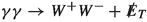

We now investigate the sensitivity that a $\gamma \gamma$ collider based on ILC or CLIC could achieve in probing the Higgs portal scenario to a dark sector discussed in the previous section above the kinematic decay threshold for $h \rightarrow S S$ (that is, for $m_S > 63$ GeV), via the process $\gamma \gamma \rightarrow W^+ W^- S S$. First, we show in Fig. 4 the (pair) production cross section of the singlet scalar S at a $\sqrt{s} = 1$ TeV ILC and a $\sqrt{s} = 3$ TeV CLIC (including the $\sqrt{s}|_{\gamma \gamma }/\sqrt{s}|_{ee} = E_{\gamma }^{\mathrm {max}}/E_{e} = 0.83$ reduction factor for $\gamma \gamma$ collisions) for the idealized luminosity spectrum from Fig. 2, as a function of the singlet scalar mass $m_S$ and for $\lambda _{HS} = 1$. We also show the corresponding $\gamma e$ production cross sections via the process $e^{+}\gamma \rightarrow W^{+} {\bar{\nu }} S S$, and include for comparison the respective production cross sections for $\sqrt{s} = 14$ TeV LHC and a future FCC-hh at $\sqrt{s} = 100$ TeV via the process $p p \rightarrow j j \,S S$. All cross sections are obtained at leading order (LO). For a 3 TeV CLIC-based $\gamma \gamma$ collider in particular, the cross section becomes much larger than that of LHC as $m_S$ increases, and is $\sim 50$ times smaller than that of FCC-hh, yet the signal cross section ratio to the SM background is much more favorable than in the latter, due to the cleaner environment of a lepton/$\gamma$ collider as compared to a hadron collider.

Considering hadronic decays for the W-bosons, the dominant SM background to the $\gamma \gamma \rightarrow W^+ W^- S S$ signal comes from triboson production $\gamma \gamma \rightarrow W^+ W^- Z$ with $Z \rightarrow \nu {\bar{\nu }}$ (see Fig. 5). Both for the 1 TeV ILC and 3 TeV CLIC analyses, we generate our signal and SM background samples at LO with MadGraph 5 [43],⁷ requiring parton-level jets to satisfy $p_T^j > 20$ GeV and $\left| \eta _j \right| < 4.5$. Generation is done for the three $\gamma \gamma$ luminosity spectra from Fig. 2. For the non-idealized spectra, we perform a fine discretization of ${{\mathcal {L}}}_{\gamma \gamma }(y)$, generate event samples for $\sqrt{s} = y$ and appropriately re-weight and combine the various samples to include the effect of the photon energy distributions f(x) in the $\gamma \gamma$ collisions (for each event, we fix the longitudinal boost in the laboratory frame via a random generation according to f(x) and the corresponding y).

Fig. 5

Example Feynman diagrams for the dominant SM background $\gamma \gamma \rightarrow W^+ W^- Z$ with $Z \rightarrow \nu {\bar{\nu }}$ in our analysis

As a final step in the initial selection, the two W-bosons from each event are reconstructed by requiring two hadronic jet pairs with invariant masses in the range $m_{jj} \in [60,\, 100]$ GeV (when multiple jet pairing choices satisfying this exist in the event, the one minimizing the difference between invariant masses of the jet pairs is chosen). For the extraction of the signal, we introduce the “missing invariant mass” $m_{\mathrm{miss}}$:

(4.1)

with $\sqrt{{\hat{s}}}$ the center-of-mass energy of the partonic collision, $E_{WW} = (m_W^2 + \left| \vec {p}_{W^+} \right| ^2)^{1/2} + (m_W^2 + \left| \vec {p}_{W^-} \right| ^2 )^{1/2}$ the energy of the $W^+W^-$ system, $p_{z_{WW}} = p_{z_{W^+}} + p_{z_{W^-}}$ the sum of longitudinal momenta of the W-bosons and the longitudinal component of the missing momentum. Both $E_{WW}$ and $p_{z_{WW}}$ can be accurately reconstructed from the hadronic W decay products. For the idealized luminosity spectrum ${{\mathcal {L}}}_{\gamma \gamma }(y) \propto \delta (y - y^{\mathrm{max}})$, knowledge of the $\gamma \gamma$ collision center-of-mass energy together with the condition (absence of longitudinal boost for the collisions in the laboratory frame) allow to very efficiently disentangle the signal from the SM background: the reconstructed events peak around $m_{\mathrm{miss}} = m_Z$ for the SM background while having a lower bound $m_{\mathrm{miss}} \ge 2\, m_S$ for the signal. A cut $m_{\mathrm{miss}} > 160$ GeV suppresses the SM background below the ${{\mathcal {O}}}(1)\%$ level, while retaining a large signal fraction for $m_S > 63$ GeV. The signal and background cross sections (for $\lambda _{HS}= 1$) for this simple cutflow are shown in Table 1. The corresponding $2\sigma$ exclusion sensitivity $S/\sqrt{B} = 2$ (with S and B the respective number of signal and background events) for $\lambda _{HS}$ as function of $m_S$ is shown in Fig. 8.

Table 1 Signal (for $\lambda _{HS}= 1$) and SM background cross sections (in fb) for the idealized luminosity spectrum ${{\mathcal {L}}}_{\gamma \gamma }(y) \propto \delta (y - y^{\mathrm{max}})$ for CLIC with $\sqrt{s}|_{ee} = 3$ TeV, after the initial event selection (4 hadronic jets with $p_T^j > 20$ GeV and $\left| \eta _j \right| < 4.5$, that are paired to reconstruct two W-bosons), and after the cut $m_{\mathrm{miss}} > 160$ GeV. The cuts are the same for ILC with $\sqrt{s}|_{ee} = 1$ TeV

Fig. 6

${{\mathcal {L}}}_{\gamma \gamma }^{nc} (y)$, $\sqrt{s}|_{ee} = 3$ TeV events. Normalized $\Delta \phi _{WW}$ distribution for the SM background (orange) and $m_S = 200$ GeV signal (red). The selection cut $\Delta \phi _{WW} < 1$ is also shown (dashed-black line)

For the non-idealized luminosity spectra, $\sqrt{{\hat{s}}}$ is not known, and neither is the longitudinal boost of each collision in the laboratory frame. Yet, the above strategy is still useful, but needs to be preceded by an event selection to increase the signal significance, since the $m_{\mathrm{miss}}$ reconstruction is degraded in this case. Focusing on ${{\mathcal {L}}}_{\gamma \gamma }^{nc} (y)$ and $\sqrt{s}|_{ee} = 3$ TeV for concreteness we show in Fig. 6 the angular separation of the two hadronic Ws in the transverse plane $\Delta \phi _{WW}$, for the SM background and $m_s = 200$ GeV signal. The clear difference between signal and background is due to the different spin nature of the intermediate particle (h vs Z) and we select events with $\Delta \phi _{WW} < 1$. After this selection, we show in Fig. 7 (top) the momentum of the hardest W-boson $\left| \vec {p}_{W_1}\right|$ vs the rapidity difference between Ws, $\Delta \eta _{WW}$. For the signal (right) the two variables are heavily correlated, and we require $R_{XY} \equiv (c_{\theta } X + s_{\theta } Y)^2/r_1^2 + (s_{\theta } X - c_{\theta } Y)^2/r_2^2 < 1$, with $\theta = 0.3$, $r_1 = 3.1$, $r_2 = 1$, $X = \left| \vec {p}_{W_1}\right| / (100\,\mathrm{GeV})- c_1(m_S)$, $Y = \Delta \eta _{WW} - c_2(m_S)$. The functions $c_{1,2}(m_S)$ are fitted to the signal data, yielding: $c_1 = 9.8 - 0.41 \,m_S - 0.097 \,m_S^2$, $c_2 = 5.3 - 0.175 \,m_S - 0.042\, m_S^2$ ($m_S$ in units of 100 GeV).

Fig. 7

${{\mathcal {L}}}_{\gamma \gamma }^{nc} (y)$, $\sqrt{s}|_{ee} = 3$ TeV events. Top: $\left| \vec {p}_{W_1}\right|$ vs $\Delta \eta _{WW}$ distribution for the SM background (left) and $m_S = 200$ GeV signal (right) after $\Delta \phi _{WW}$ selection. Signal selection is shown as a dashed-black ellipse (see text for details). Bottom: $m_{\mathrm{miss}}$ vs $E_S$ distribution for the SM background (left) and $m_S = 200$ GeV signal (right) prior to the final signal region selection $m_{\mathrm{miss}} > E_S - E_0$ (depicted as a dashed-black line)

Table 2 Signal (for $\lambda _{HS}= 1$) and SM background cross sections (in fb) for the non-idealized luminosity spectrum ${{\mathcal {L}}}_{\gamma \gamma }^{nc} (y)$ for CLIC with $\sqrt{s}|_{ee} = 3$ TeV, after the initial event selection (4 hadronic jets with $p_T^j > 20$ GeV and $\left| \eta _j \right| < 4.5$, that are paired to reconstruct two W-bosons), and the subsequent signal selection steps (see text for details). The cuts are the same for ILC with $\sqrt{s}|_{ee} = 1$ TeV

Finally, we carry out the $m_{\mathrm{miss}}$ reconstruction for the surviving events. We first remark that approximating $\sqrt{{\hat{s}}}$ purely via global event kinematic variables, e.g. $\sqrt{{\hat{s}}} \sim \sqrt{s}_{\mathrm{min}}$ [64, 65] or (note that $E_S > \sqrt{s}_{\mathrm{min}}$), does not yield an acceptable $m_{\mathrm{miss}}$ reconstruction for both signal and SM background: the average difference $\sqrt{{\hat{s}}} - E_S$ is significantly larger for the signal than for the SM background, and this effect increases as $m_S$ grows. We use an averaged approximation

(4.2)

with $E_{{{\mathcal {L}}}} = 2370$ GeV corresponding to the maximum of the ${{\mathcal {L}}}^{nc}_{\gamma \gamma } (y)$ spectrum (see Fig. 2). Assuming also , we show in Fig. 7 (bottom) the resulting distribution of $m_{\mathrm{miss}}$ vs $E_S$. Figure 7 (bottom) highlights the degrading in the reconstruction of $m_{\mathrm{miss}}$ for non-idealized luminosity spectra, from the impossibility of accurately accessing $\sqrt{{\hat{s}}}$ and for each $\gamma \gamma$ collision. Still, defining the signal region as $m_{\mathrm{miss}} > E_S - E_0$ (see Fig. 7), with fitted $E_0(m_S)/\mathrm{TeV} = 2.24 - 0.117 \, m_S - 0.028\, m_S^2$ ($m_S$ in units of 100 GeV), improves the signal discrimination, particularly for large $m_S$. The signal and SM background cross sections (for $\lambda _{HS}= 1$) after each step in the signal selection are shown in Table 2 for $m_S = 75$ GeV and $m_S = 200$ GeV, for illustratory purposes.

The above analysis is repeated for the non-idealized luminosity spectrum ${{\mathcal {L}}}_{\gamma \gamma }^{c} (y)$. In each case, we compute the $2\sigma$ exclusion sensitivity $S/\sqrt{B} = 2$ for $\lambda _{HS}$ as a function of $m_S$. These sensitivities are then shown in Fig. 8. The integrated luminosity we quote in each non-idealized scenario corresponds to that of the high-energy part of the $\gamma \gamma$ spectrum, ${{\mathcal {L}}}_{\gamma \gamma }\left( y \,> 0.8 \,y^{\mathrm{max}}\right)$ (recall the discussion around Eq. (2.2)). We also show the $2\sigma$ exclusion sensitivities achievable at HL-LHC and FCC-hh via obtained respectively from [8, 15], as a comparison.⁸ In addition we depict in Fig. 8 the lowest value of $\lambda _{HS}$ compatible with a (two-step) first order EW phase transition [62] in this scenario. Figure 8 highlights that for comparable integrated luminosities, multi-TeV $\gamma \gamma$ collisions would directly probe dark sectors via the Higgs portal with precision similar to, and potentially higher than, future hadron colliders. A $\sqrt{s} = 3$ TeV - based $\gamma \gamma$ collider could cover the whole parameter space region compatible with a two-step singlet-driven strongly first-order EW phase transition that could allow for baryogenesis.

Fig. 8

$2\sigma$ sensitivity in the ($\lambda _{HS}$, $m_S$) plane of the singlet Higgs portal model, for a $\gamma \gamma$ collider based on an $e^+ e^-$ center-of-mass energy $\sqrt{s} = 1$ TeV (“ILC”) and $\sqrt{s} = 3$ TeV (“CLIC”). Different curves correspond to: ILC 500 fb$^{-1}$ with ideal ${{\mathcal {L}}}_{\gamma \gamma }$ (dashed-yellow), ILC 3 ab$^{-1}$ with ideal ${{\mathcal {L}}}_{\gamma \gamma }$ (solid-yellow), CLIC 500 fb$^{-1}$ with ideal ${{\mathcal {L}}}_{\gamma \gamma }$ (dashed-light-blue), CLIC 3 ab$^{-1}$ with ideal ${{\mathcal {L}}}_{\gamma \gamma }$ (solid-light-blue), CLIC 3 ab$^{-1}$ with ${{\mathcal {L}}}^{nc}_{\gamma \gamma }$ (solid-black) and CLIC 3 ab$^{-1}$ with ${{\mathcal {L}}}^{c}_{\gamma \gamma }$ (solid-dark-blue). We also show the $2\sigma$ sensitivity of HL-LHC (solid-red) and FCC-hh (dashed-red) via the process $p p \rightarrow j j \,S S$. The dotted-black line shows the lower threshold for a two-step 1$^{st}$ order EW phase transition, as obtained from [62]

Before concluding, we stress the possibility of further enhancing the sensitivity to Higgs portal scenarios in $\gamma \gamma$ collisions by analyzing $W^{+} W^-$ semi-leptonic and/or leptonic final states (we also stress the importance of these modes for accurately measuring the SM background and controlling its systematic uncertainty in our analysis). The contribution to the of the events from the W decays in this case however demands a different strategy to suppress SM backgrounds (e.g. the use of transverse mass variables $M_T$ and $M_{T2}$ [68, 69]), and we leave such a study for the future.

5 Conclusions

High-energy $\gamma \gamma$-colliders constitute a potential running mode of future leptonic accelerators like the ILC, CLIC or a muon collider. In this work we have shown that $\gamma \gamma$ collisions yield a powerful avenue to probe a hidden sector of Nature which interacts with the SM via the Higgs portal and lies above the on-shell Higgs production threshold ($m_S > m_h/2$). In particular, the process $\gamma \gamma \rightarrow W^+ W^- + S S$ (S being the dark scalar that interacts directly with the SM Higgs) is a very sensitive probe of the Higgs portal interactions. Using a singlet scalar extension of the SM as the simplest realization of the Higgs portal, we have obtained the region of parameter space that would be probed by $\gamma \gamma$ collisions, showing that it can cover the possibility of a strong first-order EW phase transition in the early Universe that would give rise to the observed matter-antimatter asymmetry.

Finally, we acknowledge that some of the $\gamma \gamma$-collider specifications used in this work are at present not achievable, e.g. the combination of the luminosities assumed here with $\kappa ^{\mathrm{max}} \approx 4.83$. These depend on the future available technology by the time of its construction. Yet, we stress that the aim of this work is to show the potential of a $\gamma \gamma$-collider as a probe of the Higgs portal to a dark sector, under potentially achievable (even if not completely realistic with present technology) conditions.

Appendix A: Numerical fit to the photon energy distributions f(x)

The ansatz for the photon energy distributions f(x) used in our numerical fit of the $\gamma \gamma$ luminosity spectra uses a combination of elementary functions (which can be integrated analytically) with free coefficients. For the luminosity spectrum without multiple Compton scattering and beamstrahlung effects, ${{\mathcal {L}}}_{\gamma \gamma }^{nc}\left( y\right)$, our $f^{nc}(x)$ ansatz is given explicitly by

$$\begin{aligned} f^{nc}(x)= & {} c_0 + c_1 x + c_2 x^2 + c_3\, e^{4 x} x^2 + c_4 \, e^{6 x} x^2\nonumber \\&+ c_5 \, e^{6 x} x^4 \, . \end{aligned}$$

(A.1)

The coefficients $c_i$ are numerically fitted to satisfy Eq. (2.3) for the luminosity spectrum ${{\mathcal {L}}}_{\gamma \gamma }^{nc}\left( y\right)$, and their specific values are given by:

$$\begin{aligned} c_0 = 0.121469\, , \, c_1 = - 0.13283 \, , \, c_2 = - 0.505607 , \nonumber \\ c_3 = 0.252713 \, , \, c_4 = - 0.0838651 \, , \, c_5 = 0.0669501.\nonumber \\ \end{aligned}$$

(A.2)

For the luminosity spectrum ${{\mathcal {L}}}_{\gamma \gamma }^{c}\left( y\right)$, which includes the effect at low energies from multiple Compton scatterings and beamstrahlung fitted from [38], our $f^c(x)$ ansatz is given explicitly by

$$\begin{aligned} f^{c}(x) = f^{nc}(x) + d_0 \frac{(x^{{\mathrm{max}}} - x)^5}{x^{d_1}} \, , \end{aligned}$$

(A.3)

with the values of the coefficients $d_i$ required to fit ${{\mathcal {L}}}_{\gamma \gamma }^{c}\left( y\right)$ given by

$$\begin{aligned} d_0 = 0.124\, , \, d_1 = 0.69 \, . \end{aligned}$$

(A.4)

References

B. Patt, F. Wilczek, Higgs-field portal into hidden sectors. arXiv:hep-ph/0605188
G. Bertone, D. Hooper, J. Silk, Particle dark matter: evidence, candidates and constraints. Phys. Rep. 405, 279–390 (2005). arXiv:hep-ph/0404175
V. Silveira, A. Zee, SCALAR PHANTOMS. Phys. Lett. B 161, 136–140 (1985)
J. McDonald, Gauge singlet scalars as cold dark matter. Phys. Rev. D 50, 3637–3649 (1994). arXiv:hep-ph/0702143
C.P. Burgess, M. Pospelov, T. ter Veldhuis, The minimal model of nonbaryonic dark matter: a singlet scalar. Nucl. Phys. B 619, 709–728 (2001). arXiv:hep-ph/0011335
S. Profumo, M.J. Ramsey-Musolf, G. Shaughnessy, Singlet Higgs phenomenology and the electroweak phase transition. JHEP 08, 010 (2007). arXiv:0705.2425
J.R. Espinosa, T. Konstandin, F. Riva, Strong electroweak phase transitions in the standard model with a singlet. Nucl. Phys. B 854, 592–630 (2012). arXiv:1107.5441
D. Curtin, P. Meade, C.-T. Yu, Testing electroweak baryogenesis with future colliders. JHEP 11, 127 (2014). arXiv:1409.0005
C.-Y. Chen, J. Kozaczuk, I.M. Lewis, Non-resonant collider signatures of a singlet-driven electroweak phase transition. JHEP 08, 096 (2017). arXiv:1704.05844
J.R. Espinosa, B. Gripaios, T. Konstandin, F. Riva, Electroweak baryogenesis in non-minimal composite Higgs models. JCAP 1201, 012 (2012). arXiv:1110.2876
J.M. Cline, K. Kainulainen, Electroweak baryogenesis and dark matter from a singlet Higgs. JCAP 1301, 012 (2013). arXiv:1210.4196
D.E. Morrissey, M.J. Ramsey-Musolf, Electroweak baryogenesis. New J. Phys. 14, 125003 (2012). arXiv:1206.2942
J.M. Cline, K. Kainulainen, P. Scott, C. Weniger, Update on scalar singlet dark matter. Phys. Rev. D 88, 055025 (2013). arXiv:1306.4710] (Erratum: Phys. Rev. D 92(3), 039906 (2015))
J.A. Casas, D.G. Cerdeño, J.M. Moreno, J. Quilis, Reopening the Higgs portal for single scalar dark matter. JHEP 05, 036 (2017). arXiv:1701.08134
N. Craig, H.K. Lou, M. McCullough, A. Thalapillil, The Higgs portal above threshold. JHEP 02, 127 (2016). arXiv:1412.0258
FCC , A. Abada et al., FCC-hh: The Hadron Collider. Eur. Phys. J. ST 228(4), 755–1107 (2019)
T. Golling et al., Physics at a 100 TeV pp collider: beyond the Standard Model phenomena. CERN Yellow Rep. (3), 441–634 (2017). arXiv:1606.00947
ILC , G. Aarons et al., International Linear Collider Reference Design Report Volume 2: Physics at the ILC. arXiv:0709.1893
The International Linear Collider Technical Design Report-Volume 1: Executive Summary. arXiv:1306.6327
The International Linear Collider Technical Design Report-Volume 2: Physics. arXiv:1306.6352
CLICdp, CLIC , T.K. Charles et al., The Compact Linear Collider (CLIC)-2018 Summary Report. arXiv:1812.06018
J.M. No, M. Spannowsky, Signs of heavy Higgs bosons at CLIC: An \(e^+ e^-\) road to the electroweak phase transition. Eur. Phys. J. C 79(6), 467 (2019). arXiv:1807.04284
J. de Blas et al., The CLIC Potential for New Physics. CERN Yellow Report Monographs 3/2018 (2018). arXiv:1812.02093
Z. Chacko, Y. Cui, S. Hong, Exploring a dark sector through the Higgs portal at a lepton collider. Phys. Lett. B 732, 75–80 (2014). arXiv:1311.3306
M. Ruhdorfer, E. Salvioni, A. Weiler, A global view of the off-shell Higgs portal. SciPost Phys. 8, 027 (2020). arXiv:1910.04170
D. Buttazzo, D. Redigolo, F. Sala, A. Tesi, Fusing vectors into scalars at high energy lepton colliders. JHEP 11, 144 (2018). arXiv:1807.04743
C. Bartels, M. Berggren, J. List, Characterising WIMPs at a future \(e^+e^-\) linear collider. Eur. Phys. J. C 72, 2213 (2012). arXiv:1206.6639
M. Habermehl, M. Berggren, J. List, WIMP dark matter at the international linear collider. Phys. Rev. D 101(7), 075053 (2020). arXiv:2001.03011
CLICdp , J.-J. Blaising, P. Roloff, A. Sailer, U. Schnoor, Physics performance for Dark Matter searches at \(\sqrt{s}=\) 3 TeV at CLIC using mono-photons and polarised beams. arXiv:2103.06006
I.F. Ginzburg, G.L. Kotkin, V.G. Serbo, V.I. Telnov, Production of high-energy colliding gamma gamma and gamma e beams with a high luminosity at Vlepp accelerators. JETP Lett. 34, 491–495 (1981) (Pisma Zh. Eksp. Teor. Fiz.34,514(1981))
I.F. Ginzburg, G.L. Kotkin, V.G. Serbo, V.I. Telnov, Colliding gamma e and gamma gamma beams based on the single pass accelerators (of Vlepp Type). Nucl. Instrum. Methods 205, 47–68 (1983)
I.F. Ginzburg, G.L. Kotkin, S.L. Panfil, V.G. Serbo, V.I. Telnov, Colliding gamma e and gamma gamma Beams Based on the Single Pass e+ e- Accelerators. 2. Polarization effects. Monochromatization improvement. Nucl. Instrum. Methods A219, 5–24 (1984)
V.I. Telnov, Principles of photon colliders. Nucl. Instrum. Methods A 355, 3–18 (1995)
V.I. Telnov, Ultimate luminosities and energies of photon colliders. AIP Conf. Proc. 397(1), 259–273 (1997). arXiv:physics/9706003
V.I. Telnov, Gamma gamma, gamma-electron colliders, in Proceedings, 17th International Conference on High-Energy Accelerators, HEACC 1998: Dubna, Russian Federation, September 07–12, 1998, p. 88–93. arXiv:hep-ex/9810019
V.I. Telnov, Problems of multi-TeV photon colliders. Nucl. Instrum. Methods A 472, 280–290 (2001). arXiv:hep-ex/0012047
V.I. Telnov, Photon collider at TESLA. Nucl. Instrum. Methods A 472, 43–60 (2001). arXiv:hep-ex/0010033
H. Burkhardt, V.I. Telnov, CLIC 3-TeV photon collider option. CERN-SL-2002-013-AP, CLIC-NOTE-508 (2002)
ECFA/DESY Photon Collider Working Group , B. Badelek et al., TESLA: The Superconducting electron positron linear collider with an integrated X-ray laser laboratory. Technical design report. Part 6. Appendices. Chapter 1. Photon collider at TESLA. Int. J. Mod. Phys. A 19, 5097–5186 (2004). arXiv:hep-ex/0108012
CLIC Physics Working Group , E. Accomando et al., Physics at the CLIC multi-TeV linear collider, in Proceedings, 11th International Conference on Hadron spectroscopy (Hadron 2005): Rio de Janeiro, Brazil, August 21-26, 2005 (2004). arXiv:hep-ph/0412251
J.Q. Yu, H.Y. Lu, T. Takahashi, R.H. Hu, Z. Gong, W.J. Ma, Y.S. Huang, C.E. Chen, X.Q. Yan, Creation of electron–positron pairs in photon–photon collisions driven by 10-PW laser pulses. Phys. Rev. Lett. 122(1), 014802 (2019). arXiv:1805.04707
I.F. Ginzburg, G.L. Kotkin, Photon collider for energies 1-2 TeV. arXiv:2006.14938
J. Alwall, R. Frederix, S. Frixione, V. Hirschi, F. Maltoni, O. Mattelaer, H.S. Shao, T. Stelzer, P. Torrielli, M. Zaro, The automated computation of tree-level and next-to-leading order differential cross sections, and their matching to parton shower simulations. JHEP 07, 079 (2014). arXiv:1405.0301
W. Kilian, T. Ohl, J. Reuter, WHIZARD: simulating multi-particle processes at LHC and ILC. Eur. Phys. J. C 71, 1742 (2011). arXiv:0708.4233
W. Kilian, S. Brass, T. Ohl, J. Reuter, V. Rothe, P. Stienemeier, M. Utsch, New Developments in WHIZARD Version 2.6, in International Workshop on Future Linear Collider (LCWS2017) Strasbourg, France, October 23–27, 2017 (2018). arXiv:1801.08034
K. Kajantie, M. Laine, K. Rummukainen, M.E. Shaposhnikov, Is there a hot electroweak phase transition at m(H) larger or equal to m(W)? Phys. Rev. Lett. 77, 2887–2890 (1996). arXiv:hep-ph/9605288
F. Csikor, Z. Fodor, J. Heitger, Endpoint of the hot electroweak phase transition. Phys. Rev. Lett. 82, 21–24 (1999). arXiv:hep-ph/9809291
C. Caprini et al., Science with the space-based interferometer eLISA. II: gravitational waves from cosmological phase transitions. JCAP 04, 001 (2016). arXiv:1512.06239
C. Caprini et al., Detecting gravitational waves from cosmological phase transitions with LISA: an update. JCAP 03, 024 (2020). arXiv:1910.13125
M. Quiros, Finite temperature field theory and phase transitions, in ICTP Summer School in High-Energy Physics and Cosmology, 1 (1999). arXiv:hep-ph/9901312
S.P. Martin, Taming the goldstone contributions to the effective potential. Phys. Rev. D 90(1), 016013 (2014). arXiv:1406.2355
J. Elias-Miro, J.R. Espinosa, T. Konstandin, Taming infrared divergences in the effective potential. JHEP 08, 034 (2014). arXiv:1406.2652
J.M. Cline, P.-A. Lemieux, Electroweak phase transition in two Higgs doublet models. Phys. Rev. D 55, 3873–3881 (1997). arXiv:hep-ph/9609240
M.E. Carrington, The effective potential at finite temperature in the Standard Model. Phys. Rev. D 45, 2933–2944 (1992)
P.B. Arnold, O. Espinosa, The Effective potential and first order phase transitions: Beyond leading-order. Phys. Rev. D 47, 3546 (1993). arXiv:hep-ph/9212235 (Erratum: Phys. Rev. D 50, 6662 (1994))
H.H. Patel, M.J. Ramsey-Musolf, Stepping into electroweak symmetry breaking: phase transitions and Higgs phenomenology. Phys. Rev. D 88, 035013 (2013). arXiv:1212.5652
S. Weinberg, Perturbative calculations of symmetry breaking. Phys. Rev. D 7, 2887–2910 (1973)
L. Dolan, R. Jackiw, Gauge invariant signal for gauge symmetry breaking. Phys. Rev. D 9, 2904 (1974)
N.K. Nielsen, On the gauge dependence of spontaneous symmetry breaking in gauge theories. Nucl. Phys. B 101, 173–188 (1975)
I.J.R. Aitchison, C.M. Fraser, Gauge invariance and the effective potential. Ann. Phys. 156, 1 (1984)
H.H. Patel, M.J. Ramsey-Musolf, Baryon washout, electroweak phase transition, and perturbation theory. JHEP 07, 029 (2011). arXiv:1101.4665
D. Curtin, P. Meade, H. Ramani, Thermal resummation and phase transitions. Eur. Phys. J. C 78(9), 787 (2018). arXiv:1612.00466
M.J. Ramsey-Musolf, The electroweak phase transition: a collider target. JHEP 09, 179 (2020). arXiv:1912.07189
P. Konar, K. Kong, K.T. Matchev, \(\sqrt{{\hat{s}}}_{min}\): a global inclusive variable for determining the mass scale of new physics in events with missing energy at hadron colliders. JHEP 03, 085 (2009). arXiv:0812.1042
P. Konar, K. Kong, K.T. Matchev, M. Park, RECO level \(\sqrt{s}_{min}\) and subsystem \(\sqrt{s}_{min}\): improved global inclusive variables for measuring the new physics mass scale in \(E_T\) events at hadron colliders. JHEP 06, 041 (2011). arXiv:1006.0653
J. Heisig, M. Krämer, E. Madge, A. Mück, Probing Higgs-portal dark matter with vector-boson fusion. JHEP 03, 183 (2020). arXiv:1912.08472
CMS Collaboration, Search for invisible decays of a Higgs boson produced through vector boson fusion at the High-Luminosity LHC. CMS-PAS-FTR-18-016 (2018)
C. Lester, D. Summers, Measuring masses of semiinvisibly decaying particles pair produced at hadron colliders. Phys. Lett. B 463, 99–103 (1999). arXiv:hep-ph/9906349
A. Barr, C. Lester, P. Stephens, m(T2): the truth behind the glamour. J. Phys. G 29, 2343–2363 (2003). arXiv:hep-ph/0304226
J. Ellis, TikZ-Feynman: Feynman diagrams with TikZ. Comput. Phys. Commun. 210, 103–123 (2017). arXiv:1601.05437
Acknowledgements
J. M. N. thanks Ennio Salvioni for useful comments on the manuscript. Feynman diagrams were drawn using TikZ-Feynman [70]. J. M. N. was supported by Ramón y Cajal Fellowship contract RYC-2017-22986, and also acknowledges support from the Spanish MINECO’s “Centro de Excelencia Severo Ochoa” Programme under grant SEV-2016-0597, from the European Union’s Horizon 2020 research and innovation programme under the Marie Sklodowska-Curie grant agreement 860881 (ITN HIDDeN) and from the Spanish Proyectos de I\(+\)D de Generación de Conocimiento via grant PGC2018-096646-A-I00. A. G.-A. thanks the MICIU, for his grant within the “Garantía Juvenil” program.
Author information
Authors and Affiliations
Corresponding author