
Abstract
We describe a systematic method to construct arbitrary highest-weight modules, including arbitrary finite-dimensional representations, for any finite dimensional simple Lie algebra \({\mathfrak {g}}\). The Lie algebra generators are represented as first order differential operators in \(\frac{1}{2} \left( \dim {\mathfrak {g}} - \text {rank} \, {\mathfrak {g}}\right) \) variables. All rising generators \(\mathbf{e}\) are universal in the sense that they do not depend on representation, the weights enter (in a very simple way) only in the expressions for the lowering operators \(\mathbf{f}\). We present explicit formulas of this kind for the simple root generators of all classical Lie algebras.
Avoid common mistakes on your manuscript.
1 Introduction
Groups and algebras play a distinguished role in modern physics, since they describe symmetries. Lie groups and algebras [1, 2] are of special importance, since they underlie the structure of fundamental physics in the framework of the Standard model [3]. However, the progress at the end of the previous century reveals that the true symmetries of the stringy models involve also affine [4] and double affine algebras [5,6,7,8,9,10,11,12], which are clever generalization of the simple Lie algebras. The most straightforward approach to them is in terms of vertex operators [13, 14], which realize particular representations through the relevantly defined/deformed creation and annihilation operators – also known as “free fields”. The main goal of this paper is to give an exhaustive description of this construction in the case of ordinary Lie algebras – what will then allow to reformulate various questions (like the algebra of representations, Weyl reflections, duality/triality transformations etc.) in these terms, and discuss more interesting generalizations to other algebras on this solid basis. The main difference from the earlier considerations like in [15] will be generic formulas for all simple root generators in all finite-dimensional representation for the four classical series A, B, C and D. They represent the generators as first-order differential operators, depending on \(\frac{1}{2} \left( \dim {\mathfrak {g}} - \text {rank} \, {\mathfrak {g}}\right) \) variables – it is the case when all the Casimir operators reduce to numbers (less variables are not sufficient to describe all finite-dimensional representations, while for more variables the Casimirs become fully fledged differential operators). In affine case the variables and differential operators are promoted to chiral free fields, and are used in the free-field realization of Kac–Moody algebras in [16, 17]. In the optimal case the c-number Casimirs turn into screening operators [18, 19], which makes the free-field description of conformal theories [13] more involved and interesting. We will provide a more detailed description of affine and other generalizations elsewhere.
All the main features of these monomial representations can be seen from the simplest example of the following well-known highest-weight representation of \({\mathfrak {sl}}_2\):
Note, that \(\mathbf{h }\, \text {and}\, \mathbf{f }\) generators have a polynomial part and a part that contains a differential operator. The irreducible monomial representations have the following nice properties:
-
The monomial representation describes all finite dimensional irreducible highest weight representations in a simple and unified way. In the particular example (1), for \(\lambda \in {\mathbb {Z}}_{\geqslant 0}\) one gets irreducible \(\left( \lambda + 1\right) \)-dimensional representation \(V_{\lambda }\) with basis \(\left( 1, X,\ldots , X^{\lambda } \right) \) and \(\lambda \) is actually the Dynkin label. However, in general case, \(\lambda \in {\mathbb {R}}\) corresponds to infinite dimensional Verma module with basis \(\left( 1, X, X^2, X^3, \ldots \right) \);
-
Lie algebra generators in the monomial representation have simple form: the first order differential operators with polynomial coefficients in \(\frac{1}{2} \left( \dim {\mathfrak {g}} - \text {rank} \, {\mathfrak {g}} \right) \) variable. In the particular example of \({\mathfrak {sl}}_2\) one variable is used;
-
The Casimir operators are numbers in these monomial representations, as it should be in the irreducible representations. In the case of \({\mathfrak {sl}}_2\) there is only one Casimir operator:
$$\begin{aligned} \mathbf{C }_2 = \mathbf{e } \, \mathbf{f } + \mathbf{f } \, \mathbf{e } + \frac{1}{2} \mathbf{h }^2 = \lambda + \frac{\lambda ^2}{2}. \end{aligned}$$(2) -
The raising operators (\(\mathbf{e }\) in our notation) do not depend on the highest weight \(\lambda \) of the representation. In other words, these operators have the same form in all irreducible representations of the algebra \({\mathfrak {g}}\) and the corresponding formulas do not contain the Dynkin labels of the highest weight. The lowering operators (\(\mathbf{f }\) respectively) depend rather simply on the highest weight: only the coefficient in front of the polynomial part depends on it. As a simple consequence, the highest vector of any representation can be chosen in the following form:
$$\begin{aligned} |0\rangle _{\lambda } = 1. \end{aligned}$$(3) -
One can compute characters using the formulas for the monomial representations. The answers are the quantum dimensions. For example we provide the character of the fundamental representation \(\lambda = 1\) using (1):
$$\begin{aligned} \text {ch}_{V_{\lambda }}(\epsilon )= & {} \hbox {Tr}_{V_{\lambda }} \exp { \epsilon \mathbf{h } } = \left. \hbox {Tr}_{V_{\lambda }} \exp { \epsilon \left( \lambda - 2 X \frac{\partial }{\partial X} \right) } \right| _{\lambda = 1} \nonumber \\= & {} e^{\epsilon } + e^{-\epsilon }. \end{aligned}$$(4)It is well known that the quantum dimensions for the algebra \({\mathfrak {sl}}_2\) are the symmetric Schur polynomials \(s_{\lambda }(x_1,x_2)\) at the special point \(x_1 = e^{\epsilon }, x_2 = e^{-\epsilon }\), where \(\epsilon \) is proportional to the sum of positive roots.
-
One can consider tensor product of two irreducible representations. We provide example of highest weights \(\lambda _X\) and \(\lambda _Y\):
$$\begin{aligned} \Delta (\mathbf{e })= & {} \partial _X + \partial _Y\nonumber \\ \Delta (\mathbf{h })= & {} \lambda _X +\lambda _Y -2X\partial _X-2Y\partial _Y\nonumber \\ \Delta (\mathbf{f })= & {} \lambda _X X +\lambda _Y Y-X^2\partial _X-Y^2\partial _Y. \end{aligned}$$(5)These operators acts on the space \(V_{\lambda _X} \otimes V_{\lambda _Y}\). The highest vectors \(|0\rangle \) are described by the following equation:
$$\begin{aligned} \Delta (\mathbf{e }) |0\rangle =0. \end{aligned}$$(6)The solutions corresponding to finite dimensional representations are \((X-Y)^k\), where \( 0 \leqslant k \leqslant \text {min}(\lambda _X,\lambda _Y)\). For k not obeying the restriction, one gets the Verma module. For example, in the case \(\lambda _X=2,\, \lambda _Y=1\) one gets the representation \(V_{\lambda _X} \otimes V_{\lambda _Y}=\langle 1, X, X^2, Y, X Y , X^2 Y \rangle \) the highest vectors are 1 and \(X-Y\).
Realizations of Lie algebras in terms of differential operators are discussed in two recent papers of Libor Křižka and Petr Somberg [20, 21]. Similarly to the present paper, these works provide an explicit realizations of Lie algebras in terms of finite number of Weyl pairs \(\{ x_i, \partial _{x_i} \}\). The variables \(x_i\) can be considered as the coordinates on the corresponding (generalized) flag manifold. Its dimension is equal to the number of the Weyl pairs.
It is natural to consider two Lie algebra realizations as equivalent if they are connected by non-degenerate change of variables. On the other hand, if two realizations contain different number of variables they possesses different properties and can only be connected by some reduction.
The paper [21] provides explicit realization of non-semisimple Lie algebras. The used approach has many common features with the methods that we use in the study. Namely, the number of used variables is equal to the number of generalized root spaces \(\frac{1}{2} \left( \dim {\mathfrak {g}} - \text {rank} \, {\mathfrak {g}} \right) \). Also, the generators in [21] contain parts of \({\mathfrak {sl}}_2\) type \(\{ \partial _t, -2 t \partial _t, -t^2 \partial _t \}\), that is one of the main features of the our approach.
In the paper [20] the case of classical A-series is considered. Namely, the generators of \({\mathfrak {sl}}_{n + 2}\) \(( n \in {\mathbb {N}} )\) are realized in terms of \(2n + 1\) variables, that are coordinates on the generalized flag manifold. In particular, these formulas appears to be useful in classifying singular vectors and analysis of singular vectors in Cauchy–Riemann case of generalised flag manifolds. In contrast, our formulas for \({\mathfrak {sl}}_{n+1}\) are written in terms of \(\frac{1}{2} \left( \dim {\mathfrak {sl}}_{n + 1} - \text {rank} \, {\mathfrak {sl}}_{n + 1} \right) = \frac{n(n+1)}{2}\) and describe all finite dimensional representations in a unified way. On the language of corresponding flag manifolds, our variables are the coordinates on the usual complete flag manifold. In this paper we do not use flag structures and leave corresponding questions for future studies.
2 Simple Lie algebras
In this section we list basic facts from the theory of simple Lie algebras. Let r be the rank of a simple Lie algebra \({\mathfrak {g}}\). We construct \({\mathfrak {g}}\) using the Chevalley basis consisting of the Cartan generators \(\mathbf{h }_i\), generators \(\mathbf{e }_i\) corresponding to positive simple roots, and those corresponding to negative simple roots, \(\mathbf{f }_i\), where \(i=1,\ldots ,r\). The commutation relations in the Chevalley basis have the following form:
where \({\mathcal {A}}_{ij}\) is the Cartan matrix, i.e. an integral \(n\times n\) matrix such that \({\mathcal {A}}_{ii}=2\), \({\mathcal {A}}_{ij}<0\), \({\mathcal {A}}_{ij}=0 \Leftrightarrow {\mathcal {A}}_{ji}=0\) and \({\mathcal {A}}\) is positive definite. \({\mathcal {A}}_{ij}\) can be defined using the Killing form \(\langle \cdot , \cdot \rangle \), which is ad-invariant symmetric bilinear form:
where \(\alpha _i\) are positive simple roots.
The remaining positive and negative roots \(\Delta _{\pm }\) are obtained by the adjoint action of the simple roots on themselves. To correctly reproduce the non-simple roots one should take into account the Serre relations:
Note that in our notation the commutation relations and the Serre relations involve transposed Cartan matrix. An irreducible finite dimensional representation is completely characterized by its highest weight \(\lambda \). It is convenient to expand \(\lambda \) in the basis of fundamental weights \(\omega _i\) defined by:
where \(i,j = 1, \ldots , r\). The expansion coefficients in this basis are called Dynkin labels. The Dynkin labels of an arbitrary highest weight have the form:
The Dynkin labels of the fundamental weights are \(\omega _i = (0,\ldots ,1_i,\ldots , 0)\), where \(i=1,\ldots ,r\). To describe the highest weights of the irreducible representations we use Dynkin labels, so the formulas explicitly depend on \(\lambda _i, \ i=1,\ldots , r\).
2.1 Explicit formulas for the classical Lie algebras
In the following sections we present explicit formulas for the each series of the classical Lie algebras. We provide basic facts about their dimensions, ranks, the numbers of positive roots and Cartan matrices. The monomial representations are constructed via the variables \(X_{i,j}\) with two indices. The number of such variables and the range of the indices i, j are specific to each case. We provide formulas only for the simple roots, while the other elements of the algebra can be constructed through the adjoint action of the simple roots on themselves, which is described by (7) and (9). Note, that the formulas we get for different series are essentially similar.
One important point should be emphasized: whenever the upper summation limit is less than the lower one, then we define the sum to be vanishing.
2.2 \(\text {A}_n\) series
This series makes sense for \(n \geqslant 1\) and corresponds to classical Lie algebras \({\mathfrak {sl}}_{n+1}\):
The polynomial representations are written in terms of the variables \(X_{i,j}\), where \(n \geqslant i \geqslant j > 0\). The total number of variables is \(\sum _{i=1}^{n} i = \frac{n(n+1)}{2} = |\Delta _{+}|\) . The simple roots have the following form for \(k = n-1,\ldots , 0\):
2.3 \(\text {B}_{n}\) series
This series makes sense for \(n \geqslant 2\) and corresponds to the classical Lie algebras \(\mathfrak {so}_{2n+1}\):
The polynomial representations are written in terms of the variables \(X_{i,j}\), where \(n \geqslant i >0 \) and \(2i - 1 \geqslant j > 0\). The total number of variables is \(\sum _{i=1}^{n} 2i - 1 = n^2 = |\Delta _{+}|\) . The simple roots have the following form for \(k = n-1,\ldots , 0\):
2.4 \(\text {C}_n\) series
This series makes sense for \(n \geqslant 2\) and corresponds to the classical Lie algebras \(\mathfrak {sp}_{2n}\):
The polynomial representations are written in terms of the variables \(X_{i,j}\), where \(n \geqslant i >0 \) and \(2i - 1 \geqslant j > 0\). The total number of variables is \(\sum _{i=1}^{n} 2i - 1 = n^2 = |\Delta _{+}|\) . The simple roots have the following form for \(k = n-1,\ldots , 0\):
2.5 \(\text {D}_n\) series
This series makes sense for \(n \geqslant 3\) and corresponds to the classical Lie algebras \(\mathfrak {so}_{2n}\):
The polynomial representations are written in terms of the variables \(X_{i,j}\), where \(n \geqslant i > 1 \) and \(2(i - 1) \geqslant j > 0\). The total number of variables is \(\sum _{i=2}^{n} 2(i - 1) = n^2 - n = |\Delta _{+}|\) . The simple roots have the following form for \(k = n-1,\ldots , 0\):
3 Universal approach to simple Lie algebras
Except for explicit formulas, we provide general algorithm for constructing the irreducible highest weight representations of finite dimensional Lie algebras. We discuss the number of variables, the dependence of the representations on the highest weight and possible changes of variables.
3.1 The algorithm for constructing representations
In this section we introduce the algorithm to construct the representations for arbitrary simple Lie algebra \({\mathfrak {g}}\). This algorithm was used to obtain formulas for classical Lie algebras (14), (17), (20), (23). Although the formulas for the classical Lie algebras are written in terms of \(X_{i,j}\) variables, here we use different notation for simplicity: variables \(X_i\), where \(i = 1,\ldots , |\Delta _+|\).
A monomial representation of highest weight \(\lambda \) is determined by a map \(\rho _{\lambda }\) that sends states \(|v\rangle \) to polynomials. Lie algebra generators are sent to the first order differential operators. Schematically these rules read:
where \(\text {Pol} \! \left( X_1, \ldots , X_{|\Delta _{+}|} \right) \) are polynomials. The notation \(\rho _{\lambda }\) is used in this section for demonstrative purposes, although in the other places we omit the mapping \(\rho _{\lambda }\). The algorithm allow one to derive the simple root generators in arbitrary representation, while the other generators of the Lie algebra can be obtained from the simple roots. To construct the monomial representation one goes through the following stages:
-
1.
The form of the simple root generators \(\mathbf{e }_i, \mathbf{f }_i, \ i = 1, \ldots , \text {rank}\, {\mathfrak {g}}\) in the representation of the highest weight \(\lambda = \left( \lambda _1, \ldots , \lambda _{\text {rank}\, {\mathfrak {g}}} \right) \) is fixed by the following ansatz:
$$\begin{aligned} \rho _{\lambda } \left( \mathbf{e }_i \right)&=\frac{\partial }{\partial X_i} + \sum _{j=1,\, j\not =i }^{| \Delta _+|} A_{ij} \! \left( X_1, \ldots , X_{|\Delta _{+}|} \right) \frac{\partial }{\partial X_j}\nonumber \\ \rho _{\lambda } \left( \mathbf{f }_i \right)&=\lambda _i X_i - X_i^2\frac{\partial }{\partial X_i} + \sum _{j=1,\, j\not =i }^{| \Delta _+ |} B_{ij}\! \left( X_1, \ldots , X_{|\Delta _{+}|} \right) \frac{\partial }{\partial X_j}.\nonumber \\ \end{aligned}$$(26)One can see that the first distinguished part of these operators form an \({\mathfrak {sl}}_2\) subalgebra that is identical to (1). The main advantage of this ansatz is that the polynomials \(A_{ij}, B_{ij}\) have the same form in all representations \(\lambda \). The rising operators do not depend on representation, while the lowering operators depend on representation only through the first term (26).
-
2.
On the second stage we impose conditions to fix a remaining freedom of the ansatz. The highest vectors \(|0\rangle \) of the fundamental representations \(\omega _k, \ k = 1, \ldots , \text {rank} \, {\mathfrak {g}} \) are mapped to 1:
$$\begin{aligned} \rho _{\omega _k} \! \left( |0\rangle \right) = 1. \end{aligned}$$(27)For each value of \(i = \text {rank}\, {\mathfrak {g}} + 1, \ldots , |\Delta _{+}|\) we set:
$$\begin{aligned} \rho _{\omega _{\gamma (i)}} \! \left( \mathbf{f }_i |0\rangle \right) = X_i. \end{aligned}$$(28)Here the value \(\gamma (i)\) is picked up according to the following rule: for any positive root \(\mathbf{e }_j\) \(j = 1, \ldots , |\Delta _{+}|\) the value \( \rho _{\omega _{\gamma (i)}} \! \left( \mathbf{e }_j \mathbf{f }_i |0\rangle \right) \) is defined on previous steps. This rule is not necessary in general, however it significantly simplifies the construction. After this stage the representation is obtained uniquely.
-
3.
On this stage one can find the form of polynomials \(A_{ij}\), by demanding the appropriate action of \(\mathbf{e }_i\) in the fundamental representations \(\omega _j\).
-
4.
After reconstructing all \(\mathbf{e }_i\) the other states of the representation \(\omega _j\) can be obtained recursively by acting with \(\mathbf{e }_i\) on states \(|v\rangle \) provided that \(\rho _{\omega _j} \! \left( \mathbf{e }_i \! |v\rangle \right) \) is already known for all \(i = 1, \ldots , |\Delta _{+}|\). In other words, \(\rho _{\omega _j} \! \left( |v\rangle \right) \) can be determined from the following system of equations:
$$\begin{aligned} {\left\{ \begin{array}{ll} \rho _{\omega _j} \! \left( \mathbf{e }_1 \right) \rho _{\omega _j} \! \left( |v\rangle \right) = \rho _{\omega _j} \! \left( \mathbf{e }_1 \! |v\rangle \right) \\ \cdots \cdots \cdots \\ \cdots \cdots \cdots \\ \rho _{\omega _j} \! \left( \mathbf{e }_{|\Delta _+|} \right) \rho _{\omega _j} \! \left( |v\rangle \right) = \rho _{\omega _j} \! \left( \mathbf{e }_{|\Delta _+|} \! |v\rangle \right) . \end{array}\right. } \end{aligned}$$(29)The right hand sides of the equations can not be zero for all equations simultaneously. The previous stages guarantee that the \(\rho _{\omega _j} \! \left( \mathbf{e }_i \right) \) are linearly independent, so the solution is unique.
-
5.
After determining enough states on the previous stage, we can reconstruct \(\mathbf{f }_i\) by action between two known states \(\rho _{\omega _j} \! \left( |v\rangle \right) \) and \(\rho _{\omega _j} \! \left( \mathbf{f }_i |v\rangle \right) \).
3.2 Examples
We provide an example of the construction presented above in the case of \({\mathfrak {sl}}_3\). For \({\mathfrak {sl}}_3\) the root system is:

Lie algebra \({\mathfrak {sl}}_3\) has rank \(r = 2\). Representations are described by two Dynkin labels \(\left( \lambda _1, \lambda _2 \right) \). The algebra has three positive roots \(\mathbf{e }_1, \mathbf{e }_2, \mathbf{e }_3 = [\mathbf{e }_1, \mathbf{e }_2]\) and three negative roots \(\mathbf{f }_1, \mathbf{f }_2, \mathbf{f }_3 = [\mathbf{f }_2, \mathbf{f }_1]\) so we have to distribute \(X_1, X_2, X_3\) among states of the fundamental representations \(\omega _{1} = (1,0)\) and \(\omega _2 = (0,1)\). To simplify formulas we omit the mapping \(\rho \) and use the following notation for the highest vectors \(|0\rangle _{i} := \rho _{\omega _i} (|0\rangle )\). The diagrams of the fundamental representations looks as follows:

-
1.
Two simple positive and negative roots have the form:
$$\begin{aligned} \mathbf{e }_1&= \frac{\partial }{\partial X_1} + A_{12} \frac{\partial }{\partial X_2} + A_{13} \frac{\partial }{\partial X_3}\nonumber \\ \mathbf{e }_2&= A_{21} \frac{\partial }{\partial X_1} + \frac{\partial }{\partial X_2} + A_{23} \frac{\partial }{\partial X_3}\nonumber \\ \mathbf{f }_1&= \lambda _1 X_1 - X_1^2\frac{\partial }{\partial X_1} + B_{12} \frac{\partial }{\partial X_2} + B_{13} \frac{\partial }{\partial X_3} \nonumber \\ \mathbf{f }_2&= \lambda _2 X_2 + B_{21} \frac{\partial }{\partial X_1} - X_2^2 \frac{\partial }{\partial X_2} + B_{23} \frac{\partial }{\partial X_3}. \end{aligned}$$(30)To simplify notations we omit X dependence of polynomials \(A_{ij},B_{ij}\).
-
2.
The highest vectors are set to 1:
$$\begin{aligned} |0\rangle _1&= 1\nonumber \\ |0\rangle _2&= 1. \end{aligned}$$(31)There is one possible value \(i = 3 = \text {rank} \, {\mathfrak {sl}}_3 + 1 = |\Delta _{+}|\). We have to set some state to be \(X_3\). Possible yet undefined candidates are \(\mathbf{f }_3 |0\rangle _1\) or \(\mathbf{f }_3 |0\rangle _2\). They are both acceptable since all the states \(\mathbf{e }_i \mathbf{f }_3 |0\rangle _j\) are already defined:
$$\begin{aligned} \begin{aligned} \mathbf{e }_1 \mathbf{f }_3 |0\rangle _1&= \mathbf{f }_2 |0\rangle _1 = 0&\quad \mathbf{e }_1 \mathbf{f }_3 |0\rangle _2&= \mathbf{f }_2 |0\rangle _2 = X_2 \\ \mathbf{e }_2 \mathbf{f }_3 |0\rangle _1&= -\mathbf{f }_1 |0\rangle _1 = -X_1&\quad \mathbf{e }_2 \mathbf{f }_3 |0\rangle _2&= -\mathbf{f }_1 |0\rangle _2 = 0 \\ \mathbf{e }_3 \mathbf{f }_3 |0\rangle _1&= |0\rangle _1 = 1&\quad \mathbf{e }_3 \mathbf{f }_3 |0\rangle _2&= - |0\rangle _2 = -1. \\ \end{aligned} \end{aligned}$$(32)Note that one should be careful with the value of \(\lambda \) in formulas (30). One can choose \(\mathbf{f }_3 |0\rangle _2 = X_3\), while \(\mathbf{f }_3 |0\rangle _1\) is determined uniquely at the following stages of the algorithm. On this stage the diagrams of the representations read:

-
3.
To find the form of \(\mathbf{e }_1, \mathbf{e }_2\) we use the actions of the corresponding operators in the fundamental representations. These actions are clear from the diagrams and we use the following conditions:
$$\begin{aligned} \begin{aligned} \mathbf{e }_1 \mathbf{f }_2 |0\rangle _2&= 0\quad&\Rightarrow \quad A_{12}(X)&= 0\\ \mathbf{e }_1 \mathbf{f }_3 |0\rangle _2&= -\mathbf{f }_2 |0\rangle _2 = -X_2\quad&\Rightarrow \quad A_{13}(X)&= -X_2\\ \mathbf{e }_2 \mathbf{f }_1 |0\rangle _1&= 0\quad&\Rightarrow \quad A_{21}(X)&= 0\\ \mathbf{e }_2 \mathbf{f }_3 |0\rangle _2&= 0 \quad&\Rightarrow \quad A_{23}(X)&= 0.\\ \end{aligned} \end{aligned}$$(33)We have completely determined the positive simple roots:
$$\begin{aligned} \mathbf{e }_1&= \frac{\partial }{\partial X_1} -X_2 \frac{\partial }{\partial X_3}\nonumber \\ \mathbf{e }_2&= \frac{\partial }{\partial X_2} . \end{aligned}$$(34) -
4.
There is only one undetermined state \( \mathbf{f }_3 |0\rangle _1\). To determine it we need to solve the following system of equations:
$$\begin{aligned} \begin{aligned} \mathbf{e }_1 \mathbf{f }_3 |0\rangle _1&= 0 \quad \left( \frac{\partial }{\partial X_1} -X_2 \frac{\partial }{\partial X_3} \right) \left( \mathbf{f }_3 |0\rangle _1 \right) = 0 \\ \mathbf{e }_2 \mathbf{f }_3 |0\rangle _1&= \mathbf{f }_1 |0\rangle _1 = X_1 \quad \left( \frac{\partial }{\partial X_2} \right) \left( \mathbf{f }_3 |0\rangle _1 \right) = X_1 \\ \mathbf{e }_3 \mathbf{f }_3 |0\rangle _1&= |0\rangle _1 = 1 \quad \left( \frac{\partial }{\partial X_3} \right) \left( \mathbf{f }_3 |0\rangle _1 \right) = 1.\\ \end{aligned} \end{aligned}$$(35)The answer to this system reads:
$$\begin{aligned} \mathbf{f }_3 |0\rangle _1 = X_3 + X_1 X_2. \end{aligned}$$(36) -
5.
On the last step we find \(\mathbf{f }_1, \mathbf{f }_2\). To do this we again use actions of these operators in fundamental representations. Note that, \(\mathbf{f }_1, \mathbf{f }_2\) operators depend on \(\lambda \):
$$\begin{aligned} \begin{aligned} \left. \mathbf{f }_1 \left( \mathbf{f }_2 |0\rangle _2 \right) \right| _{\lambda = (0,1)}&= -X_3 \Rightarrow \quad B_{12}(X) = -X_3\\ \left. \mathbf{f }_1 \left( \mathbf{f }_3 |0\rangle _2 \right) \right| _{\lambda = (0,1)}&= 0\Rightarrow \quad B_{13}(X) = 0\\ \left. \mathbf{f }_2 \left( \mathbf{f }_1 |0\rangle _1 \right) \right| _{\lambda = (1,0)}&= \mathbf{f }_3 |0\rangle _1 = X_3 + X_1 X_2\\&\Rightarrow \quad B_{21}(X) = X_3 + X_1 X_2 \\ \left. \mathbf{f }_2 \left( \mathbf{f }_3 |0\rangle _2 \right) \right| _{\lambda = (0,1)}&= 0 \Rightarrow \quad B_{23}(X) = - X_2 X_3.\\ \end{aligned} \end{aligned}$$(37)The resulting \({\mathfrak {sl}}_3\) operators corresponding to simple roots have the following form:
$$\begin{aligned} \boxed { \begin{aligned} \mathbf{e }_1&= \frac{\partial }{\partial X_1} -X_2 \frac{\partial }{\partial X_3} \\ \mathbf{e }_2&= \frac{\partial }{\partial X_2} \\ \mathbf{f }_1&= \lambda _1 X_1 - X_1^2 \frac{\partial }{\partial X_1} - X_3 \frac{\partial }{\partial X_2} \\ \mathbf{f }_2&= \lambda _2 X_2 + \left( X_3 + X_1 X_2 \right) \frac{\partial }{\partial X_1} - X_2^2 \frac{\partial }{\partial X_2} - X_2 X_3 \frac{\partial }{\partial X_3}. \\ \end{aligned}} \end{aligned}$$(38)

We provide also the non-simple root operators. They can be obtained from the simple roots operators: \(\mathbf{e }_3 = [\mathbf{e }_1, \mathbf{e }_2], \ \mathbf{f }_3 = [\mathbf{f }_2, \mathbf{f }_1]\). The explicit form of these operators reads:
Non-simple root operators have more involved formulas and can be reconstructed from the simple ones, hence we do not provide non-simple roots.
We emphasize that the algorithm is applicable to any simple Lie algebra. For example we provide the generators of \(\text {G}_2\) algebra:
3.3 Comment on the number of variables
Every simple Lie algebra \({\mathfrak {g}}\) has \(|\Delta _{+} |\) \({\mathfrak {sl}}_2\) subalgebras. The highest weight representation can be considered as a representation of \(|\Delta _{+} |\) \({\mathfrak {sl}}_2\) subalgebras, each of which has its own highest weight. From the general theory we know, that we only need to consider the highest weights of the \({\mathfrak {sl}}_2\) subalgebras corresponding to the simple roots, as the other highest weights can be reconstructed uniquely. Each representation of \({\mathfrak {sl}}_2\) has at least one variable, so the minimal number of variables needed for the irreducible highest weight representation of \({\mathfrak {g}}\) is \(|\Delta _{+} |\): if we take less variables, the elements of the algebra will become linearly dependent. Moreover, we can’t take more variables, as it will lead to the representation becoming reducible and the reduction to the irreducible one can be done by applying some subspace constraint. For example, in \({\mathfrak {sl}}_2\) case one can construct the following representation:
This representations is not an irreducible one and has an infinite number of invariant subspaces, i.e. homogeneous polynomials. The constraint reducing to one of the subspaces can be chosen as
In the second line of Eqs. (42) one can choose any constant, but for convenience we choose it to be 1. By solving Eqs. (42) one gets
This representation is already irreducible, so further reduction is impossible.
3.4 Changing the variables
The representation we get is unique up to the diffeomorphic change of variables. This change can be performed as follows:
For example, for \({\mathfrak {sl}}_3\) one of the possible representations is:
The corresponding fundamental representations are the following:

One of the possible changes of variables is as follows:
Applying this change of variables one gets the representation:
After the change of variables the fundamental representations are:

Applying different changes of variables one can get from any distribution of variables on the diagrams of the fundamental representations to another one, but these distributions should give the consistent representations, i.e. the commutation relations in the algebra must be satisfied.
3.5 Applying the universal approach to the classical Lie algebras
In this section we discuss stable formulas (14), (17), (20), (23) for the infinite series A, B, C and D. By stability we understand the following property: the transition from n to \(n+1\) case involves only addition of new terms without a loss and changing of already existent ones.
To obtain stable formulas we choose specific form of function \(\gamma (i)\) from the second stage of the algorithm 3.1. Let \(\Delta _{+}^n\) be the set of its positive roots of a rank n algebra of some type A, B, C, D. Then the analog of (28) reads:
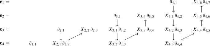
where \(k = 1, \ldots , n\). Using this rule one obtains formulas (14), (17), (20), (23). We argue that there are nice structures that arise after the renaming the variables \(X_i \rightarrow X_{a,b}\). We provide explicit formulas for rising operators where sums along lines are implied.
-
Rising operators/positive roots of \(\text {A}_5\):

-
Rising operators/positive roots of \(\text {B}_4\):

-
Rising operators/positive roots of \(\text {C}_4\):
-
Rising operators/positive roots of \(\text {D}_5\):

Note that there are strange-looking crossings in the last two operators \(\mathbf{e }_4, \mathbf{e }_5\). It corresponds to the symmetry of the \(\text {D}_n\) Dynkin diagrams – the last two “spinor” roots can be swaped.


4 Conclusion
This paper provides an explicit realization of all finite-dimensional representations of all classical Lie algebras \({\mathfrak {g}}\) in terms of differential operators in \(\frac{1}{2} \left( \dim {\mathfrak {g}} - \text {rank} \, {\mathfrak {g}}\right) \) variables. Together with the weights these are the variables which get promoted to \(\dim {\mathfrak {g}}\) free fields in the affine case, and this work can serve as a basis for deriving the Kac–Moody bosonization formulas in full generality (and not just in particular examples, as it was done in [16]). Other obvious directions include super, elliptic and DIM algebras. Remarkable simplicity of our results in the classical case raises the hope that these generalization can also be handled in a universal form for large classes of representations. This would open a way for systematic study of physical theories with DIM symmetry [7,8,9, 9,10,11,12] (like 5-brane networks [12, 22,23,24,25,26] etc.).
Every raising generator \(\mathbf{e}_{\vec \alpha }\), associated with the root \(\vec \alpha \) has a leading term \(\partial /\partial X_{\vec \alpha }\) and a number of additional terms in which other derivatives are multiplied by powers of X. They are universal, i.e. do not depend on the weights of the representation. The dependence on representation appears only in the lowering operators \(\mathbf{f}_{\vec \alpha }\), in the form of polynomials of X multiplied by the Dynkin labels. As a corollary, it shows up also in Cartan operators \(\mathbf{h}\), just as X-independent terms. Our formulas describe highest weight representations, which become also lowest weight (i.e. finite-dimensional) only for non-negative integer-valued weights. We found a general algorithm, which has a pronounced triangular structure but does not refer explicitly to Gauss or Iwasava decompositions – like it was done in [15]. Instead we get a full and explicit description for all simple algebras, which can be directly applied for practical purposes, not just to build an abstract theory. Also one can study what happens beyond the usual Dynkin diagrams, i.e. when the finite-growth restriction is raised, and analyze the problems like Vogel universality [27,28,29,30,31], which arises in the “adjoint sector”. We do not go in these directions in the present paper in order to leave it clean and transparent: classical series deserve a separate clear presentation.
Data Availability Statement
This manuscript has no associated data or the data will not be deposited. [Authors’ comment: There is no additional data to be deposited. The text contains all necessary information.]
References
M. Goto, F.D. Grosshans, Semisimple Lie algebras (1978). ISBN:0824767446. https://doi.org/10.1201/9781003071778
N. Bourbaki, Lie groups and Lie algebras (2008). ISBN:3540691715
L.B. Okun, Leptons and quarks (1980)
V.G. Kac, Infinite-Dimensional Lie Algebras, 3rd edn. (Cambridge University Press, Cambridge, 1990). https://doi.org/10.1017/CBO9780511626234
J. Ding, K. Iohara, Generalization and deformation of Drinfeld quantum affine algebras. Lett. Math. Phys. 41, 181–193 (1997). https://doi.org/10.1023/A:1007341410987
K. Miki, J. Math. Phys. 48(12), 123520 (2007). https://doi.org/10.1063/1.2823979
H. Awata et al., TheMacMahon \(R\)-matrix. JHEP 04, 097 (2019). https://doi.org/10.1007/JHEP04(2019)097. arXiv:1810.07676 [hep-th]
H. Awata et al., \((q, t)\)-KZ equations for quantum toroidal algebra and Nekrasov partition functions on ALE spaces. JHEP 03, 192 (2018). https://doi.org/10.1007/JHEP03(2018)192. arXiv:1712.08016 [hep-th]
H. Awata et al., Generalized Knizhnik–Zamolodchikov equation for Ding–Iohara–Miki algebra. Phys. Rev. D 96(2), 026021 (2017). https://doi.org/10.1103/PhysRevD.96.026021. arXiv:1703.06084 [hep-th]
H. Awata et al., Explicit examples of DIM constraints for network matrix models. JHEP 07, 103 (2016). https://doi.org/10.1007/JHEP07(2016)103. arXiv:1604.08366 [hep-th]
H. Awata et al., Toric Calabi–Yau threefolds as quantum integrable systems. \({\cal{R}}\)-matrix and \({\cal{RTT}}\) relations. JHEP 10, 047 (2016). https://doi.org/10.1007/JHEP10(2016)047. arXiv:1608.05351 [hep-th]
H. Awata et al., Anomaly in RTT relation for DIM algebra and network matrix models. Nucl. Phys. B 918, 358–385 (2017). https://doi.org/10.1016/j.nuclphysb.2017.03.003. arXiv:1611.07304 [hep-th]
A.A. Belavin, A.M. Polyakov, A.B. Zamolodchikov, Infinite conformal symmetry in two-dimensional quantum field theory. Nucl. Phys. B 241(2), 333–380 (1984). ISSN:0550-3213. https://doi.org/10.1016/0550-3213(84)90052-X
I. Frenkel, J. Lepowsky, A. Meurman, Vertex Operator Algebras and the Monster. Pure and Applied Mathematics, vol. 134 (Academic Press, New York, 1988). ISBN: 0-12-267065-5
A. Gerasimov et al., Liouville type models in group theory framework. 1. Finite dimensional algebras. Int. J. Mod. Phys. A 12, 2523–2584 (1997). https://doi.org/10.1142/S0217751X97001444. arXiv:hep-th/9601161
A. Gerasimov et al., Wess–Zumino–Witten model as a theory of free fields. Int. J. Mod. Phys. A 5, 2495–2589 (1990). https://doi.org/10.1142/S0217751X9000115X
B.L. Feigin, E.V. Frenkel, Representations of affine Kac–Moody algebras, bosonization and resolutions. Lett. Math. Phys. 19(4), 307–317 (1990). ISSN:1573-0530. https://doi.org/10.1007/BF00429950
V.S. Dotsenko, V.A. Fateev, Conformal algebra and multipoint correlation functions in 2D statistical models. Nucl. Phys. B 240(3), 312–348 (1984). ISSN:0550-3213. https://doi.org/10.1016/0550-3213(84)90269-4
A. Mironov, A. Morozov, Sh. Shakirov, Matrix model conjecture for exact BS periods and Nekrasov functions. JHEP 02, 030 (2010). https://doi.org/10.1007/JHEP02(2010)030. arXiv:0911.5721 [hep-th]
L. Křižka, P. Somberg, Algebraic analysis on scalar generalized Verma modules of Heisenberg parabolic type I.: \(A_n\)-series. Transform. Groups 22, 403–451 (2017). https://doi.org/10.1007/s00031-016-9414-5. arXiv:1502.07095 [math.RT]
L. Křižka, P. Somberg, Conformal Galilei algebras, symmetric polynomials and singular vectors. Lett. Math. Phys. 108(1), 1–44 (2017). ISSN: 1573-0530. https://doi.org/10.1007/s11005-017-0997-0. arXiv:1612.08891 [math.RT]
A. Mironov, A. Morozov, Y. Zenkevich, Ding–Iohara–Miki symmetry of network matrix models. Phys. Lett. B 762, 196–208 (2016). https://doi.org/10.1016/j.physletb.2016.09.033. arXiv:1603.05467 [hep-th]
M. Ghoneim et al., 4d higgsed network calculus and elliptic DIM algebra (2020). arXiv:2012.15352 [hep-th]
Y. Zenkevich, Higgsed network calculus. J. High Energ. Phys. 2021, 149 (2021). https://doi.org/10.1007/JHEP08(2021)149
Y. Zenkevich, \({\mathfrak{gl}}_N\) Higgsed networks (2019). arXiv:1912.13372 [hep-th]
Y. Zenkevich, Mixed network calculus (2020). arXiv:2012.15563 [hep-th]
P. Vogel, The universal Lie algebra (1999)
P. Vogel, Algebraic structures on modules of diagrams. J. Pure Appl. Algebra 215(6), 1292–1339 (2011). ISSN:0022-4049. https://doi.org/10.1016/j.jpaa.2010.08.013
A. Mironov, R. Mkrtchyan, A. Morozov, On universal knot polynomials. JHEP 02, 078 (2016). https://doi.org/10.1007/JHEP02(2016)078. arXiv:1510.05884 [hep-th]
A. Mironov, A. Morozov, Universal Racah matrices and adjoint knot polynomials: arborescent knots. Phys. Lett. B 755, 47–57 (2016). https://doi.org/10.1016/j.physletb.2016.01.063. arXiv:1511.09077 [hep-th]
A.P. Isaev, S.O. Krivonos, Split Casimir operator for simple Lie algebras, solutions of Yang -Baxter equations, and Vogel parameters. J. Math. Phys. 62, 083503 (2021). https://doi.org/10.1063/5.0049055
Acknowledgements
Our work was partly supported by the grants of the Foundation for the Advancement of Theoretical Physics “BASIS” (A.M., N.T.), by RFBR grants 19-02-00815 (A.M., Y.Z.), 20-01-00644 (N.T.), by joint RFBR grants 19-51-18006-Bolg_a (A.M., Y.Z.), 21-51-46010-CT_a (A.M., N.T., Y.Z.), 21-52-52004-MOST (A.M., Y.Z.).
Author information
Authors and Affiliations
Corresponding author
Rights and permissions
Open Access This article is licensed under a Creative Commons Attribution 4.0 International License, which permits use, sharing, adaptation, distribution and reproduction in any medium or format, as long as you give appropriate credit to the original author(s) and the source, provide a link to the Creative Commons licence, and indicate if changes were made. The images or other third party material in this article are included in the article’s Creative Commons licence, unless indicated otherwise in a credit line to the material. If material is not included in the article’s Creative Commons licence and your intended use is not permitted by statutory regulation or exceeds the permitted use, you will need to obtain permission directly from the copyright holder. To view a copy of this licence, visit http://creativecommons.org/licenses/by/4.0/.
Funded by SCOAP3
About this article

Cite this article
Morozov, A., Reva, M., Tselousov, N. et al. Irreducible representations of simple Lie algebras by differential operators. Eur. Phys. J. C 81, 898 (2021). https://doi.org/10.1140/epjc/s10052-021-09676-7
Received:
Accepted:
Published:
DOI: https://doi.org/10.1140/epjc/s10052-021-09676-7