Logarithmic expansion of field theories: higher orders and resummations

Abstract

A formal expansion for the Green’s functions of a quantum field theory in a parameter $\delta$ that encodes the “distance” between the interacting and the corresponding free theory was introduced in the late 1980s (and recently reconsidered in connection with non-hermitian theories), and the first order in $\delta$ was calculated. In this paper we study the ${\mathcal {O}}(\delta ^2)$ systematically, and also push the analysis to higher orders. We find that at each finite order in $\delta$ the theory is non-interacting: sensible physical results are obtained only resorting to resummations. We then perform the resummation of UV leading and subleading diagrams, getting the ${\mathcal {O}}(g)$ and ${\mathcal {O}}(g^2)$ weak-coupling results. In this manner we establish a bridge between the two expansions, provide a powerful and unique test of the logarithmic expansion, and pave the way for further studies.

1 Introduction

The Green’s functions ${\mathcal {G}}_n$, the main tools for calculating physical amplitudes in quantum field theory, have been approximated according to different expansions and resummations: semiclassical or $\hbar$ expansion, weak-coupling expansion, truncations of Dyson–Schwinger type, Borel-resummations, Padé approximants, resummation of infrared and ultraviolet renormalons [1,2,3,4], just to mention few well known examples.

A technique based on a non-linear expansion in a parameter $\delta$ that somehow measures the “distance” between the interacting theory and the corresponding free theory was introduced in the late 1980s [5, 6]. For a self-interacting scalar theory $(\phi ^2)^{p}$, the method consists in writing $p=1+\delta$, and then expanding the interaction term in powers of $\delta$. For generic d dimensions, the Green’s functions ${\mathcal {G}}_n$ were calculated at $O(\delta )$ in [5, 6], while the ${\mathcal {O}}(\delta ^2)$ contributions to ${\mathcal {G}}_2$ and ${\mathcal {G}}_4$ were considered in [7, 8]. This expansion was applied in particular to $(\phi ^2)^{p}$ theories in $d=4$ dimensions in [9], where it was suggested that all these theories (for any value of p) are equivalent to the $\phi ^4_4$ theory. This latter result, however, is obtained by resorting to an unconventional and (more importantly) uncontrolled renormalization scheme, where (to give an example) the coupling constant turns out to be multiplicatively renormalized and quadratically divergent. In the present work, on the contrary, we will consider the well consolidated renormalization procedure.

Needless to say, new approaches to the calculation of the ${\mathcal {G}}_n$ are of the greatest theoretical and practical interest, and the $\delta$-expansion was introduced in the hope that it could provide a new analytical tool to investigate non-perturbative phenomena, such as phase transitions, confinement, and spontaneous symmetry breaking [7]. Clearly the expansion has to be performed beyond the first order in $\delta$, and tested against known results.

These are two of the goals of the present work. We push the analysis beyond the ${\mathcal {O}}(\delta )$, studying the ${\mathcal {O}}(\delta ^2)$ systematically, and identifying for the higher orders the leading and subleading (in connection with their UV behaviour) corrections to the ${\mathcal {G}}_n$. We find that at each finite order in $\delta$ the theory is non-interacting, that is certainly not acceptable for generic spacetime dimensions and for generic interactions, and this leads us to the third goal of our work: we look for suitable resummations. By resumming leading and subleading diagrams at each order in $\delta$, we recover the weak-coupling results. This establishes a bridge between the $\delta$- and the weak-coupling expansion, provides a powerful and unique test for the $\delta$-expansion, and sets the stage for other possible resummations.

We consider a scalar theory with interaction term $\frac{g}{2} \phi ^{2p}$, that for the scopes of the $\delta$-expansion is written as $\frac{g}{2} \phi ^{2(1+\delta )}$. For $\delta =0$ the non-interacting theory is obtained, while $\delta =1$ gives the $\phi ^4$ theory: moving from $\delta =0$ to $\delta =1$, the connection between the free theory and the interacting $\phi ^4$ theory is realized.

The method starts with the logarithmic expansion [5, 6] of the interaction term

$$\begin{aligned} \frac{g}{2} \phi ^{2(1+\delta )} \,=\, \frac{g}{2} \phi ^2 \sum _{k=0}^{\infty } \frac{\delta ^k}{k!} \log ^k \phi ^2 , \end{aligned}$$

(1)

where the logs are treated with an adaptation of the replica-trick [10], and is based on the formal identity [11]:

$$\begin{aligned} \phi ^2 \log ^k \phi ^2 = \lim _{N \rightarrow 1} \frac{d^k}{dN^k} \phi ^{2N} . \end{aligned}$$

(2)

We begin our study by organizing the $\delta$-expansion in terms of Feynman diagrams that simplify the original formulation [5, 6]. We then introduce “effective vertices” in terms of which the expansion acquires a form that is essential for the purposes of the present work. Successively we study the ultraviolet (UV) behaviour of the Green’s functions by introducing a physical momentum cut-off $\Lambda$, and classify the different contributions to the ${\mathcal {G}}_n$ with respect to their dependence on $\Lambda$. We find an unexpected result: at each finite order in $\delta$, and for space-time dimensions $d>2$, the ${\mathcal {G}}_n$ with $n>2$ vanish in the UV, so that the theory appears as non-interacting.

This is a problem for the $\delta$-expansion, as for instance the $\phi ^4$ theory in $d=3$ dimensions is certainly an interacting theory. This suggests that the only way for the $\delta$-expansion to provide physically sensible results is through the resummation of diagrams that include all orders in $\delta$.

With this in mind, we begin by identifying the leading contributions to the ${\mathcal {G}}_n$ at each order in $\delta$, and then resum these terms. To our surprise, we find that such a resummation allows to recover the lowest order results of the weak-coupling expansion, and this establishes a bridge between the two expansions. Identifying and resumming subleading diagrams, we also recover the weak-coupling results at order $g^2$.

These results are new and encouraging. They show that, despite the deceptive results obtained at finite orders, the $\delta$-expansion is able to reproduce known results, and as such it is well-founded. In our opinion this means that it has great potentialities, although to find non-trivial applications further studies are needed.

The rest of the paper is organized as follows. In Sect. 2 we set up the tools for our analysis: we review the ${\mathcal {O}}(\delta )$ results [5, 6], introduce a new set of Feynman rules together with new “effective vertices”, and study the UV behaviour of the Green’s functions. In Sect. 3 we present a systematic study of the ${\mathcal {O}}(\delta ^2)$, and classify the different contributions with respect to their UV behaviour. In Sect. 4 we consider higher order contributions to the Green’s functions, and again classify them according to their UV behaviour. Section 5 is devoted to the resummation of the leading diagrams, while in Sect. 6 we proceed to the resummation of subleading terms. Section 7 is for the conclusions.

2 Expansion in $\delta$ and leading order results

In the present section we set up the tools for our analysis, showing in detail the steps for the calculation of the ${\mathcal {G}}_n$ at each order in $\delta$. As an application we calculate the first order, recovering the results of [5, 6].

We begin by introducing new Feynman diagrams (see Sect. 2.1) in terms of an auxiliary Lagrangian that simplifies the original formulation [5, 6]. The main novelty of this section, however, is the introduction of the effective vertices $\Pi _n$ (see Sect. 2.2), that at ${\mathcal {O}}(\delta )$ simply allow to write the ${\mathcal {G}}_n$ in a compact and elegant form, but become crucial for our successive analysis, when higher orders are considered.

Moreover we study the UV behaviour of the ${\mathcal {G}}_n$ with the help of a momentum cut-off $\Lambda$, and find that at ${\mathcal {O}}(\delta )$ the radiative correction to the mass is much less severe than the one obtained in weak-coupling, thus suggesting that within such an expansion the naturalness problem could be alleviated. At the same time, however, it turns out that in the UV all the Green’s function with $n \ge 4$ vanish, thus indicating that at this order the theory is non-interacting.

2.1 Definition of the theory and Feynman rules

Considering the (Euclidean) Lagrangian of a self-interacting scalar theory in d-dimensions with even interaction $\phi ^{2p}$ (p integer),

$$\begin{aligned} {\mathcal {L}} = \frac{1}{2}(\nabla \phi )^2+\frac{1}{2}m^2\phi ^2+\frac{1}{2}g\mu ^{d+(2-d)p}\phi ^{2p} , \end{aligned}$$

(3)

in the late 1980s a method for calculating the ${\mathcal {G}}_n$ was proposed [5, 6]. In a nutshell it consists in replacing the integer p with $1+\delta$ ($\delta \ge 0$), expanding the ${\mathcal {G}}_n$ as a power series in $\delta$, and assuming that at each order in $\delta$ the limit $\delta \rightarrow p-1$ provides a sensible approximation to the ${\mathcal {G}}_n$. In terms of $\delta$ Eq. (3) is written as

$$\begin{aligned} {\mathcal {L}} = \frac{1}{2}(\nabla \phi )^2+\frac{1}{2}m^2\phi ^2+\frac{1}{2}g\mu ^2\phi ^2\left( \mu ^{2-d}\phi ^2\right) ^{\delta } . \end{aligned}$$

(4)

Varying $\delta$ from zero to $p-1$, Eq. (4) “interpolates” between the free and the interacting Lagrangian. It is worth to note that, having defined the interaction term as $\phi ^2(\phi ^2)^\delta$, by varying $\delta$ we obtain theories that preserve the parity symmetry. For instance, if we consider $\delta =\frac{1}{2}$, we obtain the theory $\phi ^2 |\phi |$ rather than $\phi ^3$. This (unstable) theory would have been obtained if, rather than $\phi ^2 (\phi ^2)^\delta$ we would have considered $\phi ^2 (\phi )^{2\delta }$, so the choice $\phi ^2(\phi ^2)^\delta$ allows to implement not only the parity of the theory but also its stability.

To set up the expansion, we write $(\mu ^{2-d}\phi ^2)^\delta$ as $e^{ \delta \,\log \left( \mu ^{2-d}\phi ^2\right) }$ and expand the exponential in powers of $\log \phi ^2$:

$$\begin{aligned} {\mathcal {L}}= & {} \frac{1}{2}(\nabla \phi )^2 + \frac{1}{2}m^2\phi ^2 + \frac{1}{2}g\mu ^2\phi ^2 \nonumber \\&\times \sum _{k=0}^{\infty } \frac{\delta ^k}{k!}[ \log (\mu ^{2-d}\phi ^2)]^k. \end{aligned}$$

(5)

Including the $\delta ^0$ term in the “free Lagrangian” ${\mathcal {L}}_0$ we have

$$\begin{aligned} {\mathcal {L}}_0 \equiv \frac{1}{2}(\nabla \phi )^2 + \frac{1}{2}(m^2+g\mu ^2)\phi ^2 , \end{aligned}$$

(6)

so that the Lagrangian (5) is finally written as

$$\begin{aligned} {\mathcal {L}}= {\mathcal {L}}_0+\sum _{k=1}^\infty {\mathcal {L}}_k\equiv {\mathcal {L}}_0+ {\mathcal {L}}_{int}, \end{aligned}$$

(7)

where

$$\begin{aligned} {\mathcal {L}}_k= \frac{1}{2}g\mu ^2\phi ^2 \frac{\delta ^k}{k!}[ \log (\mu ^{2-d}\phi ^2)]^k . \end{aligned}$$

(8)

We now detail the steps that define the expansion of the ${\mathcal {G}}_n$ in powers of $\delta$, starting from (7) for defining the Feynman rules.

The partition function Z and the n-points Green’s functions are given by:

$$\begin{aligned}&Z = \int {\mathcal {D}}\phi \, e^{-\int d^du \, {\mathcal {L}}}, \end{aligned}$$

(9)

$$\begin{aligned}&{\mathcal {G}}_n(x_1,\ldots ,x_n) = \frac{1}{Z}\int {\mathcal {D}}\phi \, \phi (x_1)\ldots \phi (x_n)\, e^{-\int d^du \, {\mathcal {L}}},\nonumber \\ \end{aligned}$$

(10)

and for the even interactions that we are considering the ${\mathcal {G}}_n$ with n odd vanish.

Treating   $e^{-S_{int}}=e^{-\int d^du\, {\mathcal {L}}_{int}}$ in (9) and (10) as a perturbation, we expand this term and collect the different powers of $\delta$, thus getting

$$\begin{aligned} e^{-S_{int}}&= 1 - {\int d^du\,{\mathcal {L}}_1}+ \Bigg [-\int d^du\,{\mathcal {L}}_2 \nonumber \\&\quad +\,\frac{1}{2}\int d^du\,{\mathcal {L}}_1 \int d^dw\,{\mathcal {L}}_{1}\Bigg ] \nonumber \\&\quad + \Bigg [-\int d^du\,{\mathcal {L}}_3 +\int d^du\,{\mathcal {L}}_1 \int d^dw\,{\mathcal {L}}_2\nonumber \\&\quad -\,\frac{1}{6}\int d^du\,{\mathcal {L}}_1\int d^dw\,{\mathcal {L}}_1\int d^dz\,{\mathcal {L}}_{1}\Bigg ] + \cdots \end{aligned}$$

(11)

that is then inserted in (10).

Now comes the central feature of the method, that consists in writing each of the “interactions” $\phi ^2\log ^k (\mu ^{2-d}\phi ^2)$ in ${\mathcal {L}}_{int}$ with the help of the formal identity [11]

$$\begin{aligned} \mu ^{2-d}\phi ^2 \log ^k (\mu ^{2-d}\phi ^2) = \lim _{N \rightarrow 1} \frac{d^k}{dN^k} \mu ^{(2-d)N}\phi ^{2N} , \end{aligned}$$

(12)

that is an adaptation of the replica trick [10] to the calculation of the path integral. The method consists of the different steps listed below.

First of all the operators $\lim _{N_i\rightarrow 1}\frac{d^{k_i}}{dN_i^{k_i}}$ (for each ${\mathcal {L}}_{k_i}$ in (11) there is one of them) are moved to the left of the functional integrals. The $N_i$ are initially considered as integers, so that the calculation of the path integral is traced back to an application of the Wick’s theorem. The functions obtained after integration are then extended to real values of $N_i$, so that the derivatives with respect to $N_i$ and the limits $N_i\rightarrow 1$ can be taken.

We are interested in the calculation of the connected Green’s functions, so we can replace in (10) the partition function Z with $Z_0$, the zeroth-order (in $\delta$) approximation. From now on we refer to ${\mathcal {G}}_n$ as to the connected Green’s functions.

The procedure outlined above can be conveniently implemented by introducing a set of Feynman rules from which the diagrams corresponding to the ${\mathcal {G}}_n$ are drawn.

Neglecting for the moment the operators $\lim _{N_i\rightarrow 1}\frac{d^{k_i}}{dN_i^{k_i}}$, we begin by introducing the “auxiliary interaction Lagrangian”

$$\begin{aligned} {\mathcal {L}}^{aux}_{int}= \sum _{k=1}^\infty \lambda _{k}(N)\, \phi ^{2N} , \end{aligned}$$

(13)

where the parameters (“coupling constants”)

$$\begin{aligned} \lambda _{k}(N)\equiv \frac{1}{2} g \mu ^{2+(2-d)(N-1)} \frac{\delta ^k}{k!} , \end{aligned}$$

(14)

give rise to infinitely many 2N-legs “auxiliary vertices”

(15)

For the contribution to the ${\mathcal {G}}_n$ to a given order in $\delta$ we have to consider the connected diagrams that can be drawn to that order with the vertices (15), and then apply to each of these diagrams the operator $\lim _{N \rightarrow 1} \frac{d^k}{dN^k}$ for each vertex.

In the next section we calculate the connected Green’s functions at ${\mathcal {O}}(\delta )$, and draw the corresponding diagrams according to the Feynman rules that we have just introduced.

2.2 Green’s functions and Feynman diagrams up to ${\mathcal {O}} (\delta )$

The Green’s functions up to ${\mathcal {O}}(\delta )$ were calculated in [5, 6]. In this section, with the help of the Feynman rules given above, we introduce the effective vertices $\Pi _n$ in term of which the ${\mathcal {G}}_n$ will be conveniently written.

Let us begin by noting that, since the interaction Lagrangian contains terms that are at least ${\mathcal {O}} (\delta )$, the two-points function ${\mathcal {G}}_2(x_1,x_2)$ is the only connected Green’s function that has an order $\delta ^0$ term. We denote this contribution with ${\mathcal {G}}^{(0)}_2(x_1,x_2)$. For the free Lagrangian (6) this is nothing but the Feynman propagator (from now on $m^2+g \mu ^2\equiv M^2$)

$$\begin{aligned} {\mathcal {G}}^{(0)}_2(x_1,x_2)\equiv & {} \Delta (x_1-x_2)\nonumber \\= & {} \int \frac{d^dp}{(2\pi )^d} \frac{1}{p^2+M^2} e^{-ip(x_1-x_2)}. \end{aligned}$$

(16)

At ${\mathcal {O}} (\delta )$ we need to consider only the vertex $\lambda _1(N)$, so the contribution to the connected n-points Green’s function is (C is for connected):

$$\begin{aligned}&{\mathcal {G}}^{(1)}_n(x_1,\dots ,x_n) =\int d^du \lim _{N \rightarrow 1} \frac{d}{dN}\, \nonumber \\&\quad \times \left\{ - {\lambda _{1}(N)} \left( \frac{1}{Z_0}\int {\mathcal {D}}\phi \,e^{-S_0} \phi (x_1)\ldots \phi (x_n) \phi (u)^{2N} \right) _C \right\} ,\nonumber \\ \end{aligned}$$

(17)

where (as explained above) the derivative and the limit with respect to N are taken only once the analytic extension to real values of N is considered.

Clearly, even if at the end of the calculation we are interested in the region around $N=1$, we need an expression that is valid for all positive integers N. Actually, the path integral in (17) gives a non-vanishing result only for N integer and such that

$$\begin{aligned} N\ge \frac{n}{2}, \end{aligned}$$

(18)

as for $N<\frac{n}{2}$ no connected diagrams can be drawn (and then (17) vanishes). Under the condition (18):

(19)

where $\Delta (0)$ is the free propagator (16) for coincident space-time points, and results from each of the $N- \frac{n}{2}$ loops in the diagram in (19), while $C_n(N)$ is the combinatorial factor resulting from all the contractions:

$$\begin{aligned} C_n(N)\!=\! \left[ 2N(2N-1)\dots (2N-n\!+\!1)\right] \,(2N-n-1)!!\nonumber \\ \end{aligned}$$

(20)

In (20) the factors in the square brackets come from the contractions of n out of the 2N fields $\phi (u)$ with the n external fields $\phi (x_1)$, $\phi (x_2)$, $\dots$, $\phi (x_n)$, while the double factorial comes from the $N-\frac{n}{2}$ loops obtained with the leftover fields $\phi (u)$. Putting together all the odd factors, we can write (20) as:

$$\begin{aligned} C_n(N)= & {} 2^{\frac{n}{2}}\,\left[ N(N-1)\dots \left( N-\frac{n}{2}+1\right) \right] (2N-1)!!\nonumber \\= & {} 2^{\frac{n}{2}}\,(N)_{\frac{n}{2}}\,(2N-1)!! \end{aligned}$$

(21)

where $(x)_m$ denotes the falling factorial (for $m=0$ we define $(x)_0=1$)

$$\begin{aligned} (x)_m=x(x-1)\dots (x-m+1) \quad \forall x \in {\mathbb {R}} \ \text {and}\ m \in {\mathbb {N}}^{+}.\nonumber \\ \end{aligned}$$

(22)

From (21) we see that $C_n(N)$ vanishes for integers $N<\frac{n}{2}$, so that the last member of (19) provides the correct result for the path integral in (17) for all positive integers N. We can then use the last member of (19) to define the needed analytic extension to real values of N of the function $\varphi (N)\equiv \lambda _{1}(N)\left[ \Delta (0)\right] ^{N-\frac{n}{2}} C_n(N)$.

It is worth to observe, however, that the function analytically extended in this manner keeps memory of the fact that (19) is originally calculated for integer values of N with $N\ge \frac{n}{2}$. This is at the origin of the factor $\left[ \Delta (0)\right] ^{N-\frac{n}{2}}$ (that comes from the $N-\frac{n}{2}$ loops in (19)) that persists even after the analytic extension of $\varphi (N)$ is performed.

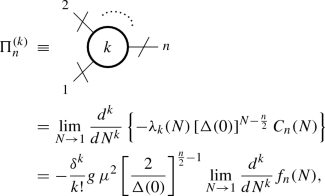
We now define the n-legs “effective vertices”

(23)

where the superscript ${}^{(1)}$ indicates that they are of ${\mathcal {O}}(\delta )$.

In terms of the $\Pi _n^{(1)}$ the ${\mathcal {O}}(\delta )$ contribution to the ${\mathcal {G}}_n$ is written as:

$$\begin{aligned} {\mathcal {G}}^{(1)}_n(x_1,\dots ,x_n) = \Pi ^{(1)}_{n} \int d^du \prod _{i=1}^{n}\Delta (x_i-u) . \end{aligned}$$

(24)

While at ${\mathcal {O}}(\delta )$ the $\Pi _n$ simply allow to write the ${\mathcal {G}}_n$ in a compact and elegant form, they are crucial for our later analysis, when the higher orders will be considered.

The calculation of $\Pi ^{(1)}_{n}$ gives

$$\begin{aligned} \Pi ^{(1)}_{n} =-\delta \,g\,\mu ^2\left[ \frac{2}{\Delta (0)}\right] ^{\frac{n}{2}-1} \lim _{N \rightarrow 1} \frac{d}{dN}\, f_n(N)\, \end{aligned}$$

(25)

where the function $f_n(N)$ of the real variable N, analytic around $N=1$, is given by:

$$\begin{aligned} f_n(N)=(N)_{\frac{n}{2}} \frac{\Gamma (N+\frac{1}{2})}{\Gamma (\frac{3}{2})} \left[ 2 \mu ^{2-d}\Delta (0)\right] ^{N-1}. \end{aligned}$$

(26)

The analytic extension (26) is obtained inserting (14) and (21) in (23), and using the identity $(2N-1)!!=2^{N-1}\frac{\Gamma (N+\frac{1}{2})}{\Gamma (\frac{3}{2})}$.

The next step consists in the calculation of the derivative of $f_n(N)$ and of the limit $N \rightarrow 1$. Due to the factor $(N-1)$ in $(N)_{\frac{n}{2}}$ of (26), for $n=4,6,\dots$, the derivative $\frac{d}{dN}f_n(N)$ has a simple behaviour for $N\rightarrow 1$. The case $n=2$ has to be treated separately. Let us begin with the latter.

$\underline{\textit{Case n=2}}.$ We have

$$\begin{aligned} f_2(N)= N \frac{\Gamma \left( N+\frac{1}{2}\right) }{\Gamma \left( \frac{3}{2}\right) } \left[ 2\mu ^{2-d}\Delta (0)\right] ^{N-1}, \end{aligned}$$

(27)

so that

$$\begin{aligned} \lim _{N \rightarrow 1} \frac{d}{dN} f_2(N)\equiv K = \log \left[ 2\mu ^{2-d}\Delta (0)\right] +1+\frac{\Gamma '(\frac{3}{2})}{\Gamma (\frac{3}{2})}, \end{aligned}$$

(28)

and the two-points effective vertex becomes

(29)

$\underline{\textit{Case n>2.}}$ In these cases $(N)_{\frac{n}{2}}$ contains the factor ${(N-1)}$, so that in the limit $N\rightarrow 1$ only the term that comes from the differentiation of the factor $(N-1)$ is non-vanishing. Indicating with $x^{(m)}$ the rising factorial $x^{(m)}=x(x+1)\dots (x+m-1)$, and noting that $(x)_m=(-1)^m\,(-x)^{(m)}$, we can write $f_n(N)$ as

$$\begin{aligned} f_n(N)= & {} N (N-1) (-1)^{\frac{n}{2}-2} (2-N)^{(\frac{n}{2}-2)} \frac{\Gamma \left( N+\frac{1}{2}\right) }{\Gamma \left( \frac{3}{2}\right) }\nonumber \\&\times \left[ 2\mu ^{2-d}\Delta (0)\right] ^{N-1} . \end{aligned}$$

(30)

Finally, being $1^{(m)}=m!$, we easily obtain:

$$\begin{aligned} \lim _{N \rightarrow 1} \frac{d}{dN} f_n(N) = (-1)^{\frac{n}{2}-2} \left( \frac{n}{2}-2\right) ! \end{aligned}$$

(31)

that in turn gives for the n-legs effective vertex $(n>2)$:

(32)

In the coming sections we will write the ${\mathcal {G}}_n$ in terms of the $\Pi _n$.

2.3 Two-points Green’s function ${\mathcal {G}}_2$

Up to order $\delta$ we have

$$\begin{aligned} {\mathcal {G}}_2(x_1,x_2)= & {} \Delta (x_1-x_2) \nonumber \\&+ \Pi ^{(1)}_{2}\int d^du \, \Delta (x_1-u)\Delta (x_2-u) . \end{aligned}$$

(33)

Going to Fourier space, and using (29) for $\Pi ^{(1)}_{2}$, we have

(34)

Equation (34) has a resemblance with the corresponding two-point Green’s function of the weak-coupling expansion up to ${\mathcal {O}}(g)$. The ${\mathcal {O}}(\delta ^0)$ term is the free propagator, while the ${\mathcal {O}}(\delta )$ contains the radiative corrections, here carried by the “loop factor” K in $\Pi ^{(1)}_{2}$.

We note that the bubble diagram in (34) is the lowest 1PI self-energy diagram within the $\delta$-expansion, and an approximation to the self-energy can be obtained by resumming the geometric series [5, 6]

(35)

that gives

$$\begin{aligned} \widetilde{{\mathcal {G}}}_2(p) = \frac{1}{p^2+M^2 + \delta g\mu ^2\,K}, \end{aligned}$$

(36)

from which the radiatively corrected mass is:

$$\begin{aligned} m_{R}^2=M^2 + \delta \, g\,\mu ^2 \left\{ \log \left[ 2\mu ^{2-d}\Delta (0)\right] +1+\frac{\Gamma '(\frac{3}{2})}{\Gamma (\frac{3}{2})}\right\} .\nonumber \\ \end{aligned}$$

(37)

Few comments are in order. The loop integral $\Delta (0)$, that is nothing but (see (16))

$$\begin{aligned} \Delta (0)=\int \frac{d^dp}{(2\pi )^d} \frac{1}{p^2+M^2} , \end{aligned}$$

(38)

diverges when $d \ge 2$, and this divergence needs to be regularized. In this respect we note that, with the exception of the Theory of Everything, any quantum field theory is an effective theory. This means that, when summing over the quantum fluctuations, we can encode our ignorance on physics above a given scale $\Lambda$ by introducing this scale in the theory as a physical momentum cut-off. This is how we regularize $\Delta (0)$.

To be more specific, let us focus on the $d=4$ case, where

$$\begin{aligned} \Delta (0)=\frac{1}{16 \pi ^2}\left( \Lambda ^2-M^2\log \frac{\Lambda ^2}{M^2}\right) +{\mathcal {O}}(\Lambda ^{-2}) . \end{aligned}$$

(39)

Replacing (39) in (37), we obtain

$$\begin{aligned} m_{R}^2= & {} M^2 + \delta g\mu ^2 \left\{ \log {\frac{\Lambda ^2}{\mu ^2}}+ 1+\frac{\Gamma '(\frac{3}{2})}{\Gamma (\frac{3}{2})} - \log (8\pi ^2) \right\} \nonumber \\&+ {\mathcal {O}}(\Lambda ^{-2}), \end{aligned}$$

(40)

from which we see that the radiative correction to the mass diverges as $\log \Lambda$, irrespectively of the value of $\delta$, i.e. irrespectively of the power in the self-interaction term $\phi ^{2+2\delta }$.

Considering in particular the ${\lambda }\phi ^4$ theory, that corresponds to the case $\delta =1$ (and also making the trivial replacement $g=\frac{\lambda }{12}$ to adhere to the usual convention), in the weak-coupling expansion the radiatively corrected mass at ${\mathcal {O}}(\lambda )$ is

$$\begin{aligned} m_R^2=m^2 + \frac{\lambda }{32\pi ^2}\left( \Lambda ^2-m^2\log {\frac{\Lambda ^2}{m^2}}\right) +{\mathcal {O}}(\Lambda ^{-2}). \end{aligned}$$

(41)

Comparing (40) with (41), it seems that within the $\delta$-expansion the unnatural quadratically divergent correction to the mass is replaced by a correction that diverges only logarithmically with $\Lambda$. If confirmed at higher orders, such a result would be of great interest for naturalness. We will further investigate this question.

2.4 Green’s functions ${\mathcal {G}}_n$ for $n>2$

As mentioned above, for $n>2$ there are no ${\mathcal {O}}(\delta ^0)$ contributions. As for the ${\mathcal {O}}(\delta )$, replacing in (24) the vertex factor (32) we obtain:

$$\begin{aligned}&{\mathcal {G}}^{(1)}_n(x_1,\ldots ,x_n)=(-1)^{\frac{n}{2}-1}\left( \frac{n}{2}-2\right) !\, \delta g\mu ^2\nonumber \\&\quad \times \left[ \frac{2}{\Delta (0)}\right] ^{\frac{n}{2}-1} \int d^du \prod _{i=1}^{n}\Delta (x_i-u) . \end{aligned}$$

(42)

Sticking again on the $d=4$ case, from (39) and (42) (moving to momentum space) we see that the amputated Green’s functions in the UV vanish as inverse powers of $\Lambda$ irrespectively of $\delta$:

$$\begin{aligned} \widetilde{{\mathcal {G}}}_n(p_1,\ldots ,p_n) \sim \frac{1}{\Lambda ^{n-2}}. \end{aligned}$$

(43)

Therefore, starting from $n=4$, all the Green’s functions vanish in the UV, thus showing that at this order in $\delta$ the theory is non-interacting. Similar results hold for any $d\ge 2$.

Two important questions came out from the analysis of the present section: the degree of divergence of the radiative correction to the mass (naturalness) and the vanishing of the Green’s functions with $n>2$ (non-interacting theory). We would like to further investigate these issues and to this end we have to move to higher orders in $\delta$. In the next section we begin with the ${\mathcal {O}}(\delta ^2)$.

3 Green’s functions and Feynman diagrams at ${\mathcal {O}}(\delta ^2)$

Let us consider now he Green’s functions at second order in $\delta$. The two- and four-points Green’s functions at this order were already considered [8], but here we perform the calculation of all the ${\mathcal {G}}_n$.

The ${\mathcal {O}}(\delta ^2)$ contributions to the ${\mathcal {G}}_n$ come from the third and fourth terms of (11). This can be read in terms of the Feynman rules for the auxiliary vertices defined in (14). For each of the ${\mathcal {G}}_n$ there are two ${\mathcal {O}}(\delta ^2)$ classes of diagrams, one with a single vertex $\lambda _2$, and one with two vertices $\lambda _1$. Let us consider separately these two terms, and indicate with ${\mathcal {G}}^{(2,1)}_n$ the contribution coming from the single vertex $\lambda _2$ and with ${\mathcal {G}}^{(2,2)}_n$ the contribution coming from the two vertices $\lambda _1$.

The one-vertex contribution This contribution comes from diagrams with one vertex $\lambda _{2}(N)$ (defined in (14)):

(44)

The diagram in (44) is basically the same as the one in (19), with the difference that the ${\mathcal {O}}(\delta ^2)$ vertex $\lambda _{2}$ rather than the ${\mathcal {O}}(\delta )$ vertex $\lambda _{1}$ appears, and correspondingly the second derivative operator. The self-loops and the combinatorial factor are the same. Similarly to what we have done at ${\mathcal {O}}(\delta )$, we define the ${\mathcal {O}}(\delta ^2)$ n-legs effective vertices $\Pi ^{(2)}_{n}$:

(45)

Inserting $\lambda _{2}(N)$ and $C_n(N)$ (Eqs. (14) and (21) respectively) in (45), we have:

$$\begin{aligned} \Pi ^{(2)}_n = -\frac{\delta ^2}{2}\,g\,\mu ^2\left[ \frac{2}{\Delta (0)}\right] ^{\frac{n}{2}-1} \lim _{N \rightarrow 1} \frac{d^2}{dN^2}\, f_n(N), \end{aligned}$$

(46)

where the function $f_n(N)$ was defined in (26). Due to the presence of the factor $(N-1)$ in $C_n(N)$, once again we have to treat the $n=2$ and $n>2$ cases separately:

$$\begin{aligned} \underline{n=2}: \qquad \Pi ^{(2)}_2&= -\frac{\delta ^2}{2}\,g\,\mu ^2 \left[ K^2 - 1 + \frac{\Gamma '(\frac{3}{2})}{\Gamma (\frac{3}{2})}\right] \end{aligned}$$

(47)

$$\begin{aligned} \underline{n>2}: \qquad \Pi ^{(2)}_n&= (-1)^{\frac{n}{2} -1}\left( \frac{n}{2}-2\right) !\,\, \delta ^2 g \mu ^2 \left[ \frac{2}{\Delta (0)}\right] ^{\frac{n}{2}-1} \nonumber \\ \left( K- H_{\frac{n}{2} -2}\right) , \end{aligned}$$

(48)

where K is defined in (28), while $H_n$ stands for the n-th Harmonic number.

The contribution ${\mathcal {G}}^{(2,1)}_n$ to ${\mathcal {G}}_n$ is then:

$$\begin{aligned} {\mathcal {G}}^{(2,1)}_n(x_1,\dots ,x_n)= \Pi _n^{(2)} \int d^du \prod _{i=1}^{n}\Delta (x_i-u). \end{aligned}$$

(49)

The two-vertex contribution This contribution is more complicated to calculate than the previous one. We will see that, due to the presence of two vertices $\lambda _{1}$, it receives contributions from an infinite number of diagrams.

From (11) we see that at this order in $\delta$ the contribution to ${\mathcal {G}}_n$ is:

$$\begin{aligned}&{\mathcal {G}}^{(2,2)}_n(x_1,\dots ,x_n)= \frac{1}{2} \int d^du\, d^dw\, \lim _{N \rightarrow 1} \, \lim _{M \rightarrow 1} \, \frac{d}{dN} \, \frac{d}{dM}\, \nonumber \\&\quad \times \Bigg \{ \left( -\lambda _{1}(N)\right) \left( -\lambda _{1}(M)\right) \,\nonumber \\&\quad \times \left( \frac{1}{Z_0} \int {\mathcal {D}}\phi \,e^{-S_0} \phi (x_1)\ldots \phi (x_n) \phi (u)^{2N} \phi (w)^{2M}\right) _C \Bigg \}. \end{aligned}$$

(50)

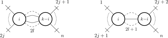
To find the diagrams that arise from (50), let us consider the contractions of the n external fields $\phi (x_1),\dots ,\phi (x_n)$ with the fields $\phi (u)$ and $\phi (w)$, connecting r of them ($0 \le r \le n$) with $\phi (u)$, and leaving the remaining $n-r$ fields for contractions with $\phi (w)$. For each of these choices, we have to consider all the diagrams obtained by connecting the two vertices u and w, while the (possibly) leftover fields are contracted in pairs (see the diagrams in (51) and (55) below). The number of possible links $u-w$ and the number of self-loops are constrained by the number of available fields, and this depends on N and M. Moreover, in order to obtain self-loops, the number of $u-w$ links must have the same parity of r. For this reason, the even ($r=2j$) and odd ($r=2j+1$) cases have to be treated separately.

“Even” contribution As for the ${\mathcal {O}}(\delta )$ case, the path integral in (50) gives non-vanishing results only for sufficiently large values of the integers N and M, namely for $N>j$ and $M>\frac{n}{2}-j$ (for any fixed j), otherwise connected diagrams cannot be drawn. Indicating with ${\mathcal {G}}^{(2,2)}_{n,\,E}$ (E is for even) the sum of all the diagrams of this kind, we have:

(51)

where $C_{n,j,l}(M,N)$ contains all the combinatorial factors, and it is easy to see that

$$\begin{aligned} C_{n,j,l}(M,N)=\frac{1}{(2l)!}\,C_{2j+2l}(N)\,C_{n-2j+2l}(M), \end{aligned}$$

(52)

while $\left( {\begin{array}{c}n\\ 2j\end{array}}\right)$ corresponds to the permutations of the external points in the diagrams. As remarked above, the actual values of N and M limit the sum over l, and the upper limit is ${Min}\equiv min(N-j,M-\frac{n}{2}+j)$. However from (21), (22), and (52) we see that the coefficient $C_{n,j,l}(M,N)$ vanishes for $l>Min$, so that the sum over l can be extended up to infinity ¹.

With this observation, and using (14), (21), and (52), the sum over l in the last member of (51) can be written as:

$$\begin{aligned}&\sum _{l=1}^{{\infty }} \left[ -\delta g\mu ^2\left( \frac{2}{\Delta (0)}\right) ^{j+l-1} f_{2j+2l}(N)\right] \nonumber \\&\quad \times \left[ -\delta g\mu ^2\left( \frac{2}{\Delta (0)}\right) ^{\frac{n}{2}-j+l-1} f_{n-2j+2l}(M)\right] \frac{\Delta (u-w)^{2l}}{(2l)!},\nonumber \\ \end{aligned}$$

(53)

where $f_m$ is defined in (26).

Even if the result in (53) was obtained for N and M integers such that $N>j$ and $M>\frac{n}{2}-j$, it is actually valid for all positive integers, due to the vanishing of the factorials in the functions $f_{2j+2l}(N)$ and $f_{n-2j+2l}(M)$ when $N\le j$ and $M\le \frac{n}{2}-j\,$. It can then be extended to real values of N and M and reinserted in (51). Performing in each of the two square brackets of (53) the derivatives and the limits with respect to N and M term by term, we recognise the effective vertices $\Pi ^{(1)}_{2j+2l}$ and $\Pi ^{(1)}_{n-2j+2l}$, so that for ${\mathcal {G}}^{(2,2)}_{n,\,E}$ we obtain:

(54)

where, in the diagrammatic representation of the last line, the factor $\frac{1}{(2l)!}$ of the first line is recovered once the indistinguishability of the 2l lines connecting the effective vertices $\Pi ^{(1)}$ in u and w is taken into account.

“Odd” contribution We now consider the case where the two vertices are joined with an odd number of lines. Indicating this contribution with ${\mathcal {G}}^{(2,2)}_{n,\,O}$ (O is for odd), we have ²:

(55)

Performing similar steps to those done for the even case, ${\mathcal {G}}^{(2,2)}_{n,\,O}$ turns out to be:

(56)

Summing up (49), (54) and (56), we finally get the whole ${\mathcal {O}}(\delta ^2)$ contribution to ${\mathcal {G}}_n^{(2)}$. We have thus obtained an elegant and compact form for ${\mathcal {G}}^{(2)}_n$, expressed in terms of the effective vertices $\Pi ^{(1)}_n$ and $\Pi ^{(2)}_n$ and of loop integrals.

We now proceed with the resummation of the series over l in Eqs. (54) and (56). The case $n=2$ has to be treated separately from the others, and we get:

$$\begin{aligned}&{\mathcal {G}}^{(2,2)}_{2,\,E} = \frac{\delta ^2}{3} g^2\mu ^4 \Delta (0) \int d^du_1 d^du_2\,\, \nonumber \\&\quad \times \left[ 3\, K\, z \,-\, z^2 \, {}_3F_2\left( 1,1,2;\, \frac{5}{2}, 3;\, z\right) \right] \nonumber \\&\quad \times \Delta (x_1-u_1) \Delta (x_2-u_1) \end{aligned}$$

(57)

$$\begin{aligned}&{\mathcal {G}}^{(2,2)}_{2,\,O} = \frac{\delta ^2}{3} g^2\mu ^4 \Delta (0) \int d^du_1 d^du_2\,\, \nonumber \\&\quad \times \left[ 3\, K^2\sqrt{z} \,+\, 2\,z^{\frac{3}{2}} \, {}_3F_2\left( 1,1,1;\, \frac{5}{2}, 2; \,z\right) \right] \nonumber \\&\quad \times \Delta (x_1-u_1) \Delta (x_2-u_2). \end{aligned}$$

(58)

Similarly, for the even Green’s functions with $n\ge 4$, the resummation gives:

$$\begin{aligned}&{\mathcal {G}}^{(2,2)}_{n,\,E} = \frac{2\delta ^2}{3} g^2\mu ^4 (-1)^{\frac{n}{2}+1} \left[ \frac{2}{\Delta (0)}\right] ^{\frac{n}{2}-2} \Gamma \left( \frac{n}{2}\right) \nonumber \\&\quad \times \int d^du_1 d^du_2\,\, \left[ 3\,K \,z - \frac{n}{2} z^2 \, {}_3F_2\left( 1,1,\frac{n}{2} +1;\, \frac{5}{2} , 3;\, z\right) \right] \, \nonumber \\&\quad \times \prod _{i=1}^{n} \Delta (x_i-u_2)+ 2\delta ^2 g^2\mu ^4 (-1)^{\frac{n}{2}} \left[ \frac{2}{\Delta (0)}\right] ^{\frac{n}{2}-2} \Gamma \left( \frac{n}{2}-1\right) \nonumber \\&\quad \times \int d^du_1 d^du_2\,\, z \, {}_3F_2\left[ \left( 1,1,\frac{n}{2} -1\right) ; \left( \frac{3}{2} , 2\right) ; z\right] \prod _{i=1}^{2} \Delta (x_i-u_1)\nonumber \\&\quad \times \prod _{k=3}^{n} \Delta (x_k-u_2) + \text {perm.}\nonumber \\&\quad + \frac{\delta ^2}{2} g^2\mu ^4 (-1)^{\frac{n}{2}} \left[ \frac{2}{\Delta (0)}\right] ^{\frac{n}{2}-2} \sum _{j=2}^{\frac{n}{2}-2} \Gamma \left( j-1\right) \Gamma \left( \frac{n}{2}-j-1\right) \nonumber \\&\quad \times \int d^du_1 d^du_2 \left[ {}_2F_1\left( j-1,\frac{n}{2} -j-1; \frac{1}{2} ; z\right) - 1\right] \nonumber \\&\quad \times \prod _{i=1}^{2j} \Delta (x_i-u_1) \prod _{k=2j+1}^{n} \Delta (x_k-u_2) + \text {perm.} \end{aligned}$$

(59)

$$\begin{aligned}&{\mathcal {G}}^{(2,2)}_{n,\,O} = \frac{2\delta ^2}{3} g^2\mu ^4 (-1)^{\frac{n}{2}} \left[ \frac{2}{\Delta (0)}\right] ^{\frac{n}{2}-2} \Gamma \left( \frac{n}{2}-1\right) \nonumber \\&\quad \times \int d^du_1 d^du_2\,\, \left[ 3\,K\,\sqrt{z} \,-\, \left( n-2\right) z^{\frac{3}{2}} \, {}_3F_2\left( 1,1,\frac{n}{2};\, \frac{5}{2}, 2;\, z\right) \right] \,\nonumber \\&\quad \times \Delta (x_1-u_1)\,\prod _{i=2}^{n} \Delta (x_i-u_2) + \text {perm.}\nonumber \\&\quad + \delta ^2 g^2\mu ^4 (-1)^{\frac{n}{2}+1} \left[ \frac{2}{\Delta (0)}\right] ^{\frac{n}{2}-2} \sum _{j=1}^{\frac{n}{2}-2} \Gamma \left( j\right) \Gamma \left( \frac{n}{2}-j-1\right) \nonumber \\&\quad \times \int d^du_1 d^du_2 \,\,\sqrt{z}\,\, {}_2F_1\left( j,\frac{n}{2} -j-1; \frac{3}{2} ; z\right) \nonumber \\&\quad \times \prod _{i=1}^{2j+1} \Delta (x_i-u_1) \prod _{k=2j+2}^{n} \Delta (x_k-u_2) + \text {perm.} \end{aligned}$$

(60)

where z is defined by:

$$\begin{aligned} z\equiv \left[ \frac{\Delta (u_1-u_2)}{\Delta (0)}\right] ^2, \end{aligned}$$

(61)

and the hypergeometric functions ${}_2 F_{1}$ and ${}_3 F_{2}$ are given by:

$$\begin{aligned}&{}_2 F_{1} (a_1,a_2; b; z) = \sum _{l=0}^{\infty } \frac{a_1^{(l)}a_2^{(l)}}{b^{(l)}} \frac{z^l}{l!};\nonumber \\&{}_3 F_{2} (a_1,a_2,a_3; b_1,b_2; z)=\sum _{l=0}^{\infty } \frac{a_1^{(l)}a_2^{(l)}a_3^{(l)}}{b_1^{(l)}b_2^{(l)}} \frac{z^l}{l!}. \end{aligned}$$

(62)

Let us note that ${}_2F_1$ and ${}_3F_2$ result from the resummation of the infinitely many diagrams (with increasing number of internal lines) in Eqs. (54) and (56). They depend on the spacetime variables $u_1$ and $u_2$ and, as long as $u_1\ne u_2$, their convergence is guaranteed, as in this case $|z|<1$ (a sufficient condition for the convergence of the series that define the hypergeometric functions). However, $z=1$ for $u_1=u_2$, and the hypergeometric functions in this case might present convergence problems. In fact, we know that, for the special case $z=1$, the function ${}_2 F_{1}$ is convergent if the condition

$$\begin{aligned} Re(b-a_1-a_2)>0 \end{aligned}$$

(63)

is fulfilled, while for the function ${}_3 F_{2}$ the convergence condition to be satisfied is

$$\begin{aligned} Re(b_1+b_2-a_1-a_2-a_3)>0. \end{aligned}$$

(64)

Applying these conditions to ${}_2 F_{1}$ and ${}_3 F_{2}$ in Eqs. (57)–(60), we find that both conditions (63) and (64) reduce to

$$\begin{aligned} n<5. \end{aligned}$$

(65)

Therefore, ${\mathcal {G}}^{(2,2)}_{2}$ and ${\mathcal {G}}^{(2,2)}_{4}$ are certainly convergent for any value of z, while for Green’s functions with $n>4$ we need to carefully consider the singularities (induced by the limit $u_1 \rightarrow u_2$) in each of the ${\mathcal {G}}^{(2,2)}_{n}$, and in particular study whether these singularities are integrable or not. We have performed this analysis for dimensions $d=3$ and $d=4$. In both cases we found that ${\mathcal {G}}^{(2,2)}_{6,\, E}$ and ${\mathcal {G}}^{(2,2)}_{6,\, O}$ have integrable singularities in $u_1=u_2$, while for $n>6$ we find more and more severe non-integrable singularities as n increases.

However, the singular contributions coming from ${\mathcal {G}}^{(2,2)}_{n,\, O}$ exactly cancel those coming from ${\mathcal {G}}^{(2,2)}_{n,\, E}$, so that no integrability problem ever shows up. Therefore, the full contribution to ${\mathcal {G}}^{(2,2)}_{n}$ does not present any convergence problem, and we have not to worry any longer on singularities that appear at intermediate steps of the calculation.

3.1 Ultraviolet behaviour of the ${\mathcal {G}}_n$ in $d=4$ dimensions

Let us specify for illustrative purposes to the case $d=4$, even though the present analysis is straightforwardly generalized to all $d\ge 2$.

One-vertex contributions From Eqs. (47)–(49) we see that at ${\mathcal {O}}(\delta ^2)$ the UV behaviour of the one-vertex contributions to the Green’s functions is entirely given by the $\Pi _n^{(2)}$, so that:

$$\begin{aligned} {\mathcal {G}}^{(2,1)}_{n} \sim {\left\{ \begin{array}{ll} \Lambda ^{2-n} \log \Lambda &{}\text {for } n\ne 2\\ \log ^2\Lambda &{}\text {for } n=2. \end{array}\right. } \end{aligned}$$

(66)

It is worth to compare (66) with the corresponding (one-vertex) contribution at ${\mathcal {O}}(\delta )$ given by the effective vertices $\Pi _n^{(1)}$ (Eqs. (29) and (32)). We see that, moving from the ${\mathcal {O}}(\delta )$ to the ${\mathcal {O}}(\delta ^2)$, the UV behaviour is enhanced by a power of $\log \Lambda$. However, as for the ${\mathcal {O}}(\delta )$, the Green’s function ${\mathcal {G}}_2$ get a divergent contribution, while for $n\ge 4$ the ${\mathcal {G}}_n^{(2,1)}$ vanish. Let us move now to the ${\mathcal {O}}(\delta ^2)$ contributions coming from two-vertex diagrams.

Two-vertex contributions The UV behaviour of the two-vertex contributions ${\mathcal {G}}^{(2,2)}_{n}$ to the Green’s functions can be read from Eqs. (54) and (56), that are written in terms of effective vertices $\Pi ^{(1)}_k$ and loop integrals. From the UV behaviour of the $\Pi ^{(1)}_k$ (that is immediately read from (29) and (32)), and from the divergence brought by the loop integrals in (54) and (56), we see that in both cases the leading diagrams are those with lowest possible number of lines connecting the two vertices. We then have:

$$\begin{aligned} {\mathcal {G}}^{(2,2)}_{n,\,E} \sim \Lambda ^{-n} \log ^2 \Lambda \qquad {\mathcal {G}}^{(2,2)}_{n,\,O} \sim {\left\{ \begin{array}{ll} \Lambda ^{2-n} \log \Lambda &{}\text {for } n\ne 2\\ \log ^2\Lambda &{}\text {for } n=2. \end{array}\right. } \end{aligned}$$

(67)

Equations (66) and (67) give the UV behaviour of the ${\mathcal {O}}(\delta ^2)$ contributions to the Green’s functions: ${\mathcal {G}}_2$ diverges, while the ${\mathcal {G}}_n$ with $n\ge 4$ vanish. Putting these results together with those obtained at ${\mathcal {O}}(\delta )$, we conclude that up to ${\mathcal {O}}(\delta ^2)$ the theory is non-interacting.

This is a somehow deceptive result. If confirmed at higher orders, it would mean that a truncation of the theory at any finite order in $\delta$ would produce vanishing transition amplitudes. Such a result cannot be accepted on general physical grounds. In fact, leaving aside the case of the $\phi ^4$ theory in $d=4$ dimensions, we know (for instance) that the same theory in $d=3$ dimensions is certainly interacting.

In order to further investigate this point we now move to the higher order contributions to the ${\mathcal {G}}_n$. The next section is devoted to this analysis.

4 Green’s functions at higher orders in $\delta$

The next step in the expansion consists in considering the ${\mathcal {O}}(\delta ^3)$. Starting from this order, however, the procedure outlined in the previous sections presents increasing difficulties. Nevertheless a restricted set of diagrams, relevant to our analysis, can be treated resorting to the same techniques previously introduced. In particular the organization of the diagrams in terms of effective vertices will be crucial to dig out their UV behaviour.

4.1 Green’s function and effective vertices

Let us consider the different cases that we face when we move to ${\mathcal {O}}(\delta ^k)$. According to the Feynman rules derived in Sect. 2, the contributions to the ${\mathcal {G}}_n$ at this order are obtained by taking all the combinations of vertices $\lambda _{i}$ such that the resulting diagrams are ${\mathcal {O}} (\delta ^k)$. Three cases have to be distinguished:

• 1. Single-vertex diagrams These diagrams are obtained when we take the vertices $\lambda _{k}$. They are practically the same as those appearing in (19) and (44), with the difference that the elementary vertex is $\lambda _{k}$ rather than $\lambda _{1}$ or $\lambda _{2}$, and that we have the k-th derivative with respect to N rather than the first or second derivative. These diagrams are immediately given in terms of the ${\mathcal {O}}(\delta ^k)$ n-legs effective vertices:

  

  (68)

  where the last member is obtained by using (14), (21) and (26). Diagrams of this kind are handled with the same techniques described before.

• 2. Two-vertex diagrams These diagrams are obtained by taking a vertex $\lambda _{i}$ and a vertex $\lambda _{k-i}$ (with $1\le i \le k-1$). They are then similar to those appearing in (51) and (55), with the difference that the elementary vertices are now $\lambda _{i}$ and $\lambda _{k-i}$ (rather than twice $\lambda _{1}$), and that the derivatives with respect to N and M are of degree i and $k-i$ (rather than first order derivatives in both cases). The analytic extension of the appropriate functions is performed in the same way followed for the ${\mathcal {O}}(\delta ^2)$. The corresponding diagrams are given in terms of the ${\mathcal {O}}(\delta ^i)$ and ${\mathcal {O}}(\delta ^{k-i})$ effective vertices, and are similar to those contained in (54) and (56) for the ${\mathcal {O}}(\delta ^2)$:

  

  (69)

• 3. Three or more vertices These diagrams are far more complicated than the previous ones. They have m vertices ($m>2$) and then $\left( {\begin{array}{c}m\\ 2\end{array}}\right)$ sums over the number of links, so that the analytic extensions become more involved than those previously considered.

From the results of the previous and present sections we see that, with the introduction of the effective vertices, the $\delta$-expansion can be organized in a compact and elegant way, as it allows to draw the Feynman diagrams in terms of the $\Pi ^{(i)}$ only. In the next section we proceed with the analysis of the UV behaviour of the ${\mathcal {G}}_n$. Again we will see that this study becomes extremely easy when performed in terms of the effective vertices.

4.2 UV behaviour of the Green’s functions

In this section we study the ultraviolet behaviour of the Green’s functions. Initially we focus on the $d=4$ dimensions case and consider diagrams with one, two and three effective vertices. Successively we move to diagrams with any number of effective vertices, and go back to generic d dimensions (from now on we use the expression “n-vertex” to indicate “n-effective vertex”).

One-vertex diagrams At ${\mathcal {O}}(\delta ^k)$ the one-vertex diagram that contributes to ${\mathcal {G}}_n$ is:

(70)

where as before we adopt the convention that for $n=2$, $\Lambda ^0$ has to be read as a power of $\log \Lambda$ in the numerator. For $n>2$ at any finite order in $\delta$ a vanishing contribution to ${\mathcal {G}}_n$ is obtained, as no power of $\log \Lambda$ can undo the suppression due to $\Lambda ^{n-2}$.

Two-vertex diagrams The diagrams with two effective vertices have the generic structure

(71)

where $r\ge 2$ is the number of lines between the vertices, and $I_r(p)$ is the multi-loop integral (p is the total momentum carried in the loop)

$$\begin{aligned}&I_r(p)\,=\,\int \frac{d^dp_1}{(2\pi )^d}\dots \frac{d^dp_{r-1}}{(2\pi )^d} \frac{1}{p^2_1+M^2}\nonumber \\&\quad \cdots \frac{1}{p^2_{r-1}+M^2}\frac{1}{(p-\sum _{i=1}^{r-1}p_i)^2+M^2}. \end{aligned}$$

(72)

In the last member of (71) we kept three distinct factors as they come from three different building blocks in the diagram: the first one comes from the effective vertex $\Pi ^{(i)}_{m+r}$, the second one from the effective vertex $\Pi ^{(k-i)}_{n-m+r}$, the third one from the loops between the two vertices. To each of these factors we apply the convention that whenever $\Lambda ^0$ appears it has to be read as a power of $\log \Lambda$ in the numerator.

Three-vertex diagrams Moving to the case of three effective vertices, the diagrams to be considered are (in configuration space):

(73)

where $m_1+m_2+m_3=n$ and $i_1+i_2+i_3=k$. Moreover, as we are taking into account only 1PI diagrams, we have either $r=0$ and $s,t\ge 2$ (and similar relations changing the roles of r, s and t) or $r,s,t,\ge 1$.

The diagram with $r\!=\!s\!=\!t\!=\!1$ (see (74) below) has a convergent triangle loop, and in terms of $\Lambda$ it goes as:

(74)

For all the other cases ($r+s+t\ge 4$), the superficial degree of divergence D of the loop integrals is non-negative, actually $D=4(r+s+t-2)-2(r+s+t)=2(r+s+t-4)\ge 0$, so that the (superficial) cut-off dependence of the generic diagram is:

(75)

In (74) and (75) we split the contribution of each of the building blocks (three effective vertices and loop integrals) in different factors, and adopt the same convention introduced below Eq. (71).

To summarize (and neglecting the subleading dependence on $\log \Lambda$ that is harmless for our scopes) the ultraviolet behaviour of the 1PI contributions to ${\mathcal {G}}_n$ with one, two and three effective vertices is given by:

• 1-vertex: $\,\sim \, \Lambda ^{2-n}$

• 2-vertices: $\,\sim \, \Lambda ^{-n}$

• 3-vertices: $\,\sim \, \Lambda ^{-n}$ (Eq. (74))    and/or   $\Lambda ^{-2-n}$ (Eq. (75)).

We then see that the leading contribution in the UV comes from the one-vertex diagrams, as it was the case for the ${\mathcal {O}}(\delta ^2)$.

Generic number V of effective vertices We can extend the previous analysis to a generic number V of effective vertices. Indicating with $N_I$ the number of internal lines, and going back to generic d dimensions, the superficial degree of divergence D of the loop integrals is:

$$\begin{aligned} D=d(N_I-V+1)-2N_I. \end{aligned}$$

(76)

Concerning the contribution of the effective vertices, we begin by noting that the total number of legs is $n+2N_I$. Therefore, writing (70) for generic d,

(77)

The contribution from the effective vertices is then:

$$\begin{aligned} \prod _{i=1}^{V} \Pi ^{(k_i)}_{m_i} \sim \prod _{i=1}^{V} \frac{\left( \log \Lambda \right) ^{k_i-1}}{\Lambda ^{\frac{d-2}{2}(m_i-2)}} \sim {\Lambda ^{\frac{2-d}{2}\left( n +2N_I-2V\right) }}, \end{aligned}$$

(78)

where in the last member of (78) we omit powers of $\log \Lambda$ as they are harmless for the scopes of the present classification.

We now have to distinguish the two cases $D\ge 0$ and $D<0$. In the first case the cut-off dependence of the diagram with n external lines, V vertices, and $N_I$ internal lines comes from both the effective vertices (78) and the loop integrals (76). In d dimensions:

$$\begin{aligned} {\Lambda ^{\frac{2-d}{2}n+d-2V}}\quad \left( \,\,\overset{d=4}{\rightarrow } \,\,{\Lambda ^{4-n-2V}}\,\right) . \end{aligned}$$

(79)

When $D<0$ the cut-off dependence comes uniquely from the effective vertices, i.e. from (78). For any fixed value of V, the condition $D<0$ is verified when $V\le N_I < \frac{d}{d-2}(V-1)$, where the lower limit comes because we are considering only 1PI diagrams. For $V=2$ the condition $D<0$ is never verified. For $V>2$ the leading diagram (the one that is less suppressed in terms of $\Lambda$) with $D<0$ is the diagram with the minimal possible $N_I$, that is $N_I=V$. It goes as:

$$\begin{aligned} {\Lambda ^{\frac{2-d}{2}n}} \quad \left( \,\,\overset{d=4}{\rightarrow } \,\, {\Lambda ^{-n}}\,\right) . \end{aligned}$$

(80)

From (77), (79), and (80) we see that the UV leading diagram (that here means the one that is less suppressed with $\Lambda$) is the diagram with $V=1$, that is the diagram in (77). This is what we have already seen at ${\mathcal {O}}(\delta )$ ($k=1$) and at ${\mathcal {O}}(\delta ^2)$ ($k=2$).

Although $\Pi _n^{(k)}$ at each order in $\delta$ (i.e. for each value of k) gives the leading contribution to ${\mathcal {G}}_n$, from (77) we see that for $\Lambda \rightarrow \infty$ it vanishes. To our dissatisfaction, we have then found that at any finite order in $\delta$ the Green’s functions with $n\ge 4$ vanish. In other words: at any finite order in $\delta$ the theory is non-interacting.

This result is obtained for any value of $d \ge 2$ and for any value of $\delta$. Needless to say, it cannot be accepted in general. For instance, if it is true that for the $\phi ^4$ ($\delta =1$) theory in four dimensions a final word on its triviality or non-triviality has still to be said, for the same theory in $d=3$ dimensions we certainly know that it is interacting.

In our opinion this “strange” behaviour of the Green’s functions comes from the truncation of the interaction term in the Lagrangian (5) to a finite power of $\log \phi ^2$ (note that when the interaction is truncated to the power $\log ^k\phi ^2$, for each of the ${\mathcal {G}}_n$ we get contributions up to ${\mathcal {O}}(\delta ^k)$). In other words, such a truncation is not sufficient to generate a non-trivial S matrix.

This clearly indicates that we cannot expect to extract sensible physical results if we restrict ourselves to a finite order in $\delta$. We can still hope to get non-vanishing physical amplitudes if we resort to resummations that include all orders in $\delta$. To this end, according to the analysis on the UV behaviour of the ${\mathcal {G}}_n$, it seems natural to start with resumming the 1PI leading contributions, that as we have seen in the present section are the one-vertex diagrams. In the next section we proceed with the resummation of these terms.

5 Resummation of the one-vertex diagrams

We now proceed to resum the one-vertex diagrams that contribute to the ${\mathcal {G}}_n$ at each order in $\delta$. As before, the cases $n=2$ and $n>2$ have to be treated separately.

5.1 Two-points Green’s function ${\mathcal {G}}_2$

According to the analysis of the previous sections, the leading contributions to ${\mathcal {G}}_2$ at each order in $\delta$ come from one-vertex diagrams and from their iterations. Going to momentum space, in Sect. 2 we have seen that the ${\mathcal {O}}(\delta )$ contribution is:

(81)

that (for $d\ge 2$) diverges as $\log \Delta (0) \sim \log \Lambda$. At order $\delta ^2$ there are two leading diagrams,

(82)

both diverging as $\log ^2 \Delta (0)$, while for the order $\delta ^3$ the leading divergences are contained in the four diagrams:

(83)

all of them diverging as $\log ^3\Delta (0)$. Similarly for the higher orders.

Our goal is to resum the diagrams whose first instances are shown in (81)–(83). We begin by resumming the diagrams with one bubble, successively those with two bubbles, and so on. The resummation of the one-bubble diagrams gives:

(84)

where the series converges due to the analyticity of the function $f_2(N)$ (defined in (27)) on the positive real axis. We finally have:

$$\begin{aligned} \Gamma _2=g\,\mu ^2 \left[ 1-(\delta +1) \frac{\Gamma (\delta +\frac{3}{2})}{\Gamma (\frac{3}{2})}\left[ 2\mu ^{2-d}\Delta (0)\right] ^{\delta }\right] . \end{aligned}$$

(85)

Equation (85) is nothing but the resummation of the 1PI diagrams $\Pi ^{(k)}_2$, whose leading UV behaviour is $\Pi ^{(k)}_2 \sim \left[ \log \Delta (0)\right] ^k\sim (\log \Lambda )^k$. From the explicit expression of $f_2(N)$ (Eq. (27)) that appear in (84) we can also see that  $\lim _{N \rightarrow 1} \frac{d^k}{dN^k} f_2(N)\sim [\log \Delta (0)]^k$, and this immediately explains why $\Gamma _2$ in (85) depends on $\Delta (0)^\delta \sim \Lambda ^{(d-2)\delta }$. The resummation then results in a stronger UV behaviour of $\Gamma _2$.

For the $\phi ^4$ theory ($\delta =1$) in $d=4$ dimensions, for instance, we have $\Gamma _2 \sim \Lambda ^2$, that is the weak-coupling expansion UV behaviour. Actually we have more than that. In this case in fact (85) becomes:

(86)

that is the weak-coupling result at first order in g for the Lagrangian (see (4), (6), (7)):

$$\begin{aligned} {\mathcal {L}}=\frac{1}{2}(\nabla \phi )^2+\frac{1}{2}M^2\phi ^2 +\left( \frac{1}{2}g\,\phi ^{4} - \frac{1}{2}g\mu ^2\phi ^2 \right) . \end{aligned}$$

(87)

We will see that this is just the first brick of a bridge between the expansion in $\delta$ and the weak-coupling expansion.³

For generic integer values of $\delta$, and generic d, rather than (86) we get:

$$\begin{aligned} \Gamma _2\,\overset{\delta \in \mathbb {Z_+}}{=}\, g \mu ^2 -(\delta +1)(2\delta +1)!!\,g \mu ^{2+(2-d)\delta }\, \Delta (0)^{\delta }, \end{aligned}$$

(88)

that is the weak-coupling result for the interacting $\phi ^{2+2\delta }$ theory in d dimensions.

Resumming the two-bubble diagrams we easily get:

(89)

and adding also the three-, four-, $\dots$ bubble diagrams, we finally obtain:

(90)

This is the main result of the present section. Sticking again on the $\phi ^4_4$ theory, (90) is nothing but the resummation of tadpole (plus crossed) diagrams in weak-coupling. More generally, i.e. for generic d and $\delta$ (even non-integers values), it is natural to call (90) the weak-coupling result for the full propagator.

Inserting (85) in (90), for the renormalized mass we get:

$$\begin{aligned} m_R^2&=M^2-\Gamma _2=m^2+2^{\delta }\,(\delta +1)\frac{\Gamma (\delta +\frac{3}{2})}{\Gamma (\frac{3}{2})}\nonumber \\&\,g \mu ^{2+(2-d)\delta }\, \Delta (0)^{\delta }. \end{aligned}$$

(91)

It is worth to note that the iterated insertions of $\Gamma _2$ in (90) provides the term $-g\mu ^2$, that combined with $M^2$ restores $m^2$ as the tree level mass term.⁴

Comparing (91) with the result for $m^2_R$ at ${\mathcal {O}}(\delta )$ (Eq. (37)), we see that the same comments made below Eq. (85) hold also for the renormalized mass: for $d > 2$ the resummation turns the logarithmic divergence of the ${\mathcal {O}}(\delta )$ to a $\Lambda ^{(d-2)\delta }$ divergence.

If we again specify to the 4-dimensional $\phi ^4$ theory, $m_R^2$ turns out to be:

$$\begin{aligned} m_R^2=m^2+\,6\,g \, \Delta (0)=m^2 + \frac{3\,g}{8 \pi ^2}\left( \Lambda ^2-M^2\log {\frac{\Lambda ^2}{M^2}}\right) , \end{aligned}$$

(92)

that coincides with the weak-coupling result (41), with the difference that in the logarithmic term $m^2$ is replaced by $M^2$ (the explanation for this difference is given in the footnote below, and is cured when higher order approximations are included).

5.2 Green’s functions ${\mathcal {G}}_n$ for $n>2$

We now consider the resummation of diagrams for Green’s functions ${\mathcal {G}}_n$ with $n>2$ along the same lines of Sect. 2.3. As already noted in Sect. 4, the diagrams for ${\mathcal {G}}_n$ with one effective vertex are leading, but there are one-particle reducible diagrams that have the same superficial cut-off dependence. As it is well known, however, their contribution is already taken into account when dealing with Green’s functions with lower n, and we then focus on the 1PIs only, i.e. on the resummation of the effective vertices. Amputating the external propagators, and factoring out the momentum conservation, for the resummed n-legs vertex functions $\Gamma _n$ we obtain:

(93)

where, as for $\Gamma _2$, the last step is allowed by the analyticity of the function $f_n(N)$ defined in (26) on the positive real axis. Due to the vanishing of the falling factorial in (26), $\,\,\forall n>2$ we have $f_n(1)=0$, so that we finally get:

$$\begin{aligned} \Gamma _n= \, -g\,\mu ^2\,\left[ \frac{2}{\Delta (0)}\right] ^{\frac{n}{2}-1} (\delta +1)_{\frac{n}{2}}\frac{\Gamma (\delta +\frac{3}{2})}{\Gamma (\frac{3}{2})}\left[ 2\mu ^{2-d}\Delta (0)\right] ^{\delta }. \end{aligned}$$

(94)

This result is obtained for generic positive real values of $\delta$. For integer $\delta$ it becomes:

$$\begin{aligned} \Gamma _n\,\overset{\delta \in \mathbb {Z_+}}{=}\,-g\,\mu ^{2+(2-d)\delta }\, 2^{\frac{n}{2}-1}(\delta +1)_{\frac{n}{2}} (2\delta +1)!! \Delta (0)^{\delta +1-\frac{n}{2}}.\nonumber \\ \end{aligned}$$

(95)

Equation (94) (or (95)) is the main result of the present section. We have been able to resum the 1PI leading diagrams of the $\delta$-expansion, getting as in 5.1 the weak-coupling result. This can be easily checked if we refer once again to the $\phi ^4_4$ theory, i.e. specifying (95) for $\delta =1$ and $d=4$:

(96)

(97)

Equation (96) shows that the resummation of the all orders four-points effective vertices $\Pi _4^{(k)}$ (that are the 1PI leading terms at each order $\delta ^k$) simply gives the tree-level vertex $-12 g$ of the weak-coupling expansion, diagrammatically represented by the last member.⁵ Moreover, while each of the $\Pi _4^{(k)}$ vanishes as $\frac{(\log \Lambda )^{k-1}}{\Lambda ^2}$, the resummation of infinite powers of $\log \Lambda$ cancels the $\Lambda ^2$ in the denominator, giving rise to the finite result (96).

Turning to (97), we see from (94) that for the present case ($\delta =1$) the falling factorial $(\delta +1)_{\frac{n}{2}}$ vanishes for $n\ge 6$. As before this coincides with the tree-level weak-coupling result, where there are no lowest order connected diagrams with $n>4$ external legs for the $\phi ^4$ theory.

The results in Eqs. (96) and (97) are at the same time welcome and deceptive. They are welcome as they confirm (see Sect. 2.3) that from the $\delta$-expansion meaningful results are obtained. They are deceptive from the viewpoint of the applications: the resummation of the leading diagrams provides nothing more than the weak-coupling tree-level results. Focusing on $\Gamma _4$, we already know that at each finite order in $\delta$ it vanishes, and here we have shown that to recover the tree-level interacting character of the theory, $\Gamma _4=-12 g$, the resummation of the leading diagrams of the $\delta$-expansion is needed.

Sections 4 and 5 show that physically sensible results can be obtained only by resorting to resummations of $\delta$-diagrams. In the present section we resummed the leading ones. In the next section we will resum subleading diagrams with two effective vertices.

6 Resummation of two-vertex diagrams

The total contribution to ${\mathcal {G}}_n$ at ${\mathcal {O}}(\delta ^k)$ ($k\ge 2$) from diagrams with two vertices is given by the sum of all the diagrams of the kind (69). We indicate it with ${\mathcal {G}}^{(k,2)}_{n}$, and consider as in Sect. 3.1 the classes of “Even” and “Odd” diagrams, according to the parity of the number of links between the two effective vertices in (69). Writing then ${\mathcal {G}}^{(k,2)}_{n}={\mathcal {G}}^{(k,2)}_{n,\,E}+{\mathcal {G}}^{(k,2)}_{n,\,O}$ we have:

(98)

and

(99)

Our goal is to perform the resummation of the two-vertex contributions: ${\mathcal {G}}^{(2v)}_{n}\equiv \sum _{k=2}^{\infty } {\mathcal {G}}^{(k,2)}_{n}$. Let us resum separately the even and odd contributions. Starting with the even ones we have:

$$\begin{aligned} {\mathcal {G}}^{(2v)}_{n,\,E}&= \frac{1}{2} \sum _{j=0}^{n/2} \sum _{l=1}^{\infty } \left\{ \sum _{k=2}^{\infty }\,\sum _{\alpha =1}^{k-1}\, \Pi ^{(\alpha )}_{2j+2l} \, \Pi ^{(k-\alpha )}_{n-2j+2l}\right\} \nonumber \\&\qquad \times \frac{1}{(2l)!} \left[ I_{2l}(x_1{,\scriptstyle \dots },x_{2j};x_{2j+1}{,\scriptstyle \dots },x_n) \right. \nonumber \\&\left. \qquad \quad +\,\, \left( {\begin{array}{c}n\\ 2j\end{array}}\right) -1 \, \mathrm{perm.}\right] . \end{aligned}$$

(100)

where

$$\begin{aligned}&I_{r}(x_1,\dots ,x_{2j};x_{2j+1},\dots ,x_n)\nonumber \\&\quad =\int d^du \, d^dw\, \prod _{i=1}^{2j}\Delta (x_i-u)\nonumber \\&\qquad \times \prod _{h=2j+1}^n \!\Delta (x_h-w) \,\, \Delta (u-w)^{r}. \end{aligned}$$

(101)

The double series in the curly brackets is nothing but the Cauchy product:

$$\begin{aligned} \sum _{k=2}^{\infty }\,\sum _{\alpha =1}^{k-1}\,\, \Pi ^{(\alpha )}_{2j+2l} \,\, \Pi ^{(k-\alpha )}_{n-2j+2l}&=\left( \sum _{\alpha =1}^{\infty }\Pi ^{(\alpha )}_{2j+2l}\right) \nonumber \\&\quad \times \left( \sum _{\beta =1}^{\infty }\Pi ^{(\beta )}_{n-2j+2l}\right) \end{aligned}$$

(102)

where $\beta =k-\alpha$, and for (102) to hold it is needed that the two series in the r.h.s. are convergent, with at least one of them absolutely convergent.

We already summed the series in the round brackets of (102) (see (85) and (94)). As they are Taylor expansions (around $x=1$) of functions that are analytic in the complex half-plane $Re(x)>-\frac{1}{2}$ (due to the presence of $\Gamma (x+\frac{1}{2})$ in (85) and (94)), their radius of convergence is $\frac{3}{2}$. Therefore the validity of (102) is guaranteed for $\delta <\frac{3}{2}$, as in this case both series in the right hand side of (102) are absolutely convergent. The possible extension of this result to larger values of $\delta$ is an interesting question that we do not pursue in this work.

For our scopes Eq. (102) is crucial as it converts the resummation of diagrams with two effective vertices in the product of series that resum one-vertex diagrams. This in turn means that the final result can be written in terms of the $\Gamma _n$ introduced in (84) and (93). For the “Even” diagrams, from (100) and (102) we have:

$$\begin{aligned}&{\mathcal {G}}^{(2v)}_{n,\,E}=\frac{1}{2} \sum _{j=0}^{n/2} \sum _{l=1}^{\infty } \frac{\Gamma _{2j+2l}\,\,\Gamma _{n-2j+2l}}{(2l)!}\nonumber \\&\quad \times \left[ I_{2l}(x_1{,\scriptstyle \dots },x_{2j};x_{2j+1}{,\scriptstyle \dots },x_n)+\left( {\begin{array}{c}n\\ 2j\end{array}}\right) -1 \, \mathrm{perm.}\right] . \end{aligned}$$

(103)

Following similar steps, an analogous result is obtained for the “Odd” contribution:

$$\begin{aligned} {\mathcal {G}}^{(2v)}_{n,\,O}&= \frac{1}{2} \sum _{j=0}^{\frac{n}{2}-1} \sum _{l=0}^{\infty } \frac{\Gamma _{2j+2l+2}\,\, \Gamma _{n-2j+2l}}{(2l+1)!}\nonumber \\&\quad \times \left[ I_{2l+1}(x_1{,\scriptstyle \dots },x_{2j+1};x_{2j+2}{,\scriptstyle \dots },x_n) \right. \nonumber \\&\quad \left. +\,\, \left( {\begin{array}{c}n\\ 2j+1\end{array}}\right) -1 \, \mathrm{perm.}\right] , \end{aligned}$$

(104)

and ${\mathcal {G}}^{(2v)}_{n}$ is finally obtained summing up (103) and (104). We note that for integer values of $\delta$ the $\Gamma _r$ in (103) and (104) are given by (88) and (95), and that for $r>2\delta +2$ they vanish (due to the vanishing of the falling factorial). As a result, the sums over l in (103) and (104) are truncated to a finite value of l.

Equations (103) and (104) result from resumming two-vertex diagrams, and we will see in a moment that they are nothing but the well known ${\mathcal {O}}(g^2)$ weak-coupling result. This is immediately seen if we stick again on the $\delta =1$ case, i.e. on the $\phi ^4$ theory, and for the sake of concreteness focus on ${\mathcal {G}}_2$ and ${\mathcal {G}}_4$.

Concerning ${\mathcal {G}}_2$, with the help of (88), (95) (for $\delta =1$) and (101), from Eqs. (103) and (104) we obtain all the ${\mathcal {O}}(g^2)$ weak-coupling diagrams:

(105)

(106)

(107)

(108)

(109)

(110)

where the first two diagrams are the two terms corresponding to $l=1$ in (103) (the only possible value of l for $\delta =1$), the successive three diagrams are the three terms corresponding to $l=0$ in (104), while the last diagram is the $l=1$ term of the latter equation. All the diagrams above are the well known second order weak-coupling diagrams for ${\mathcal {G}}_2$ of the $\phi ^4$ theory (the diagrams with the insertion of crossed vertices are due to the quadratic interaction term in the Lagrangian (87)). The third, fourth and fifth diagram are reducible (they are already considered in the geometrical series of the previous section, and are related to $\Gamma _2$) while the first, second and sixth diagram are 1PI, and provide the ${\mathcal {O}}(g^2)$ contribution to the proper self-energy.

Moving to ${\mathcal {G}}_4$, and sticking again on the $\phi ^4$ theory, we see that Eqs. (103) and (104) give rise to all the weak-coupling ${\mathcal {O}}(g^2)$ diagrams (the corresponding permutations are not explicitly written):

(111)

(112)

(113)

The first diagram corresponds to the $l=1$ term in (103) (the only non-vanishing “even” term for $\delta$=1), while the second and third diagrams correspond to the two terms with $l=0$ in (104) (for $\delta =1$ all the other “odd” terms vanish). The diagrams (112) and (113) are one-particle reducible and are related to corrections of the external propagator, while the first diagram is the genuine ${\mathcal {O}}(g^2)$ correction to ${\mathcal {G}}_4$. Although we have explicitly shown only ${\mathcal {G}}_2$ and ${\mathcal {G}}_4$, these findings are of more general validity: the resummed ${\mathcal {G}}_n$ considered are nothing but the ${\mathcal {O}}(g^2)$ weak-coupling results.

We can now summarize the results of the present and previous sections. In Sect. 5 we found that resumming the UV leading diagrams of the $\delta$-expansion (one-vertex diagrams) we obtain the weak-coupling ${\mathcal {O}}(g)$ results. In this section we resummed two-vertex diagrams, and to our surprise we found that we fall again in the weak-coupling expansion, more precisely we found the ${\mathcal {O}}(g^2)$ results.

Although these results are of no interest for practical applications, they provide a powerful test of the $\delta$-expansion, that in the past was mainly tested for space-time dimensions $d\le 1$. Here we consider the cases relevant to quantum field theory ($d\ge 2$). Needless to say, a test against known results is necessary before a new calculation technique can be safely put at work. Clearly, once this method is tested, new strategies have to be considered in order to fully exploit the potentialities of the method itself.

A technical remark concerns the delicate issue of the convergence and/or absolute convergence of the series involved in the Cauchy product in (102), where for values of $\delta >3/2$ the splitting for the double series is not guaranteed (see comments below (102)), while for $\delta <3/2$ the results are well established. In this respect, it is worth to remind that the interacting $\phi ^4$ theory considered above is obtained for $\delta =1$.

Finally we observe that, following the same lines of this section, we expect that the bridge between the $\delta$- and the weak-coupling expansions extends also to higher orders. In particular we expect that the resummation of diagrams with a generic number m of effective vertices should lead to the weak-coupling expansion results at order $g^m$.

7 Summary, conclusions and outlooks

In the present work: (i) we systematically study the ${\mathcal {O}}(\delta ^2)$ of the logarithmic expansion; (ii) extend the analysis to higher orders; (iii) analyze the UV behaviour of the Green’s functions within this expansion; (iv) perform resummations.

We begin by organizing the expansion in terms of Feynman diagrams that simplify the original formulation [5, 6], and then introduce new “effective vertices” $\Pi ^{(i)}_n$ that turn out to be essential for our analysis. As a first result we find that, at any order $\delta ^k$ in the expansion parameter $\delta$, the generic Green’s function ${\mathcal {G}}_n$ turns out to be the sum of diagrams with 1, 2, $\dots$, k effective vertices.

A crucial result of our analysis concerns the UV behaviour of the ${\mathcal {G}}_n$ at each order in $\delta$. Starting with ${\mathcal {O}}(\delta )$, we find that the Green’s functions ${\mathcal {G}}_n$ for $n\ge 4$ vanish: at this order the theory is non-interacting. Successively we move to the ${\mathcal {O}}(\delta ^2)$, and find that the theory is non-interacting even at this order. Extending then the analysis to higher orders, we finally find that the theory is non-interacting at any finite order in $\delta$.

These results carry an important message. The truncation of the interaction Lagrangian in (5) to finite powers of $\log \phi ^2$ is not sufficient to guarantee the existence of non-trivial S-matrix elements. We cannot extract physically sensible results if we restrict ourselves to finite orders in $\delta$, so that the potentialities of this expansion can be exploited only if we resort to resummations.

We begin by considering the resummation of the 1PI diagrams, that are leading with respect to their UV behaviour. These are the diagrams containing a single effective vertex $\Pi _n^{(i)}$ ($i=1,2,\dots ,\infty$). Considering the $\phi ^4$ theory, we see that such a resummation allows to recover the well-known lowest order weak-coupling results: the usual tadpole diagram for ${\mathcal {G}}_2$, simply the tree-level vertex for ${\mathcal {G}}_4$, while all the other ${\mathcal {G}}_n$ with $n \ge 6$ vanish.

The fact that to obtain the weak-coupling tree-level result (the classical vertex $-g$) for ${\mathcal {G}}_4$ we need to resum all the UV leading 1PI contributions strongly supports our argument that the truncation of the interaction Lagrangian to a finite number of powers of $\log \phi ^2$ is not strong enough to keep the interaction on: at any finite order in $\delta$ the interaction is off.

At the same time these results provide a welcome and necessary test for the $\delta$-expansion, that in the past [5, 6, 8, 11] was mainly checked for $d=0$ and $d=1$ dimensions where the integrals involved in the calculations are convergent. Our test is realized for any value of d, and in particular for $d \ge 2$, where divergent loop integrals appear. In [6] an O(N) scalar theory in the framework of the large N expansion was considered, but no reference to the UV behaviour of the ${\mathcal {G}}_n$ was made.

We next consider the two-vertex diagrams, that give subleading contributions to the ${\mathcal {G}}_n$. Resumming these terms, we find the diagrams of the weak-coupling expansion at ${\mathcal {O}}(g^2)$ (we still refer to the $\phi ^4$ theory). Compared to the resummations that lead to the ${\mathcal {O}}(g)$ results, however, here we face additional difficulties. We have to resum double series, and this requires the convergence of each of them and the absolute convergence of at least one of them. We find that when $\delta <3/2$ these requirements are fulfilled. This is very interesting, as for instance the physically relevant $\phi ^4$ theory ($\delta =1$) lies within the convergence radius.

Our analysis builds a bridge between the $\delta$-expansion and the weak-coupling expansion, thus providing a powerful and unique test for the former. These results pave the way for future applications of the $\delta$-expansion.

The present work is a step in the systematic investigation of the $\delta$-expansion. Referring to one of the main results of our analysis, namely that physically sensible results can be obtained only when appropriate resummations are considered, we think that significant improvement in this field will be achieved when we will be able to find the appropriate resummations that can take us beyond the weak coupling results. This is an open question on which we plan to come back in the future.

References

S. Coleman, Aspects of Symmetry: Selected Erice Lectures of Sydney Coleman (Cambridge University Press, Cambridge, 1985)
R.J. Rivers, Path Integral Methods in Quantum Field Theory (Cambridge University Press, Cambridge, 1987)
M.E. Peskin, D.V. Schroeder, An Introduction to Quantum Field Theory (Addison-Wesley, New York, 1995)
J. Zinn-Justin, Quantum Field Theory and Critical Phenomena (Claredon Press, Oxford, 1996)
C.M. Bender, K.A. Milton, M. Moshe, S.S. Pinsky, L.M. Simmons, Logarithmic approximations to polynomial Lagrangians. Phys. Rev. Lett. 58, 2615 (1987)
C.M. Bender, K.A. Milton, M. Moshe, S.S. Pinsky, L.M. Simmons Jr., Novel perturbative scheme in quantum field theory. Phys. Rev. D 37, 1472 (1988)
C.M. Bender, H.F. Jones, A new nonperturbative calculation: renormalization and the triviality of \(\lambda \phi ^4\) in four-dimensions field theory. Phys. Rev. D 38, 2526 (1988)
C.M. Bender, H.F. Jones, Evaluation of Feynman diagrams in the logarithmic approach to quantum field theory. J. Math. Phys. 29, 2659 (1988)
H.T. Cho, K.A. Milton, J.M. Cline, S.S. Pinsky, L.M. Simmons Jr., Triviality of monomial Higgs potentials. Nucl. Phys. B 329, 574 (1990)
M. Mezard, G. Parisi, M. Virasoro, Spin Glass Theory and Beyond (World Scientific, Singapore, 1987)
C.M. Bender, N. Hassanpour, S.P. Klevansky, S. Sarkar, PT-symmetric quantum field theory in \(D\) dimensions. Phys. Rev. D 98(12), 125003 (2018)
Acknowledgements
This work is carried out within the INFN project QFT-HEP and is supported in part by the Polish National Science Centre HARMONIA grant under contract UMO-2015/18/M/ST2/00518 (2016–2021).
Author information
Authors and Affiliations
Corresponding author
Rights and permissions
Open Access This article is licensed under a Creative Commons Attribution 4.0 International License, which permits use, sharing, adaptation, distribution and reproduction in any medium or format, as long as you give appropriate credit to the original author(s) and the source, provide a link to the Creative Commons licence, and indicate if changes were made. The images or other third party material in this article are included in the article’s Creative Commons licence, unless indicated otherwise in a credit line to the material. If material is not included in the article’s Creative Commons licence and your intended use is not permitted by statutory regulation or exceeds the permitted use, you will need to obtain permission directly from the copyright holder. To view a copy of this licence, visit http://creativecommons.org/licenses/by/4.0/.
Funded by SCOAP3
About this article
Cite this article
Branchina, V., Chiavetta, A. & Contino, F. Logarithmic expansion of field theories: higher orders and resummations. Eur. Phys. J. C 81, 535 (2021). https://doi.org/10.1140/epjc/s10052-021-09293-4
Received:
Accepted:
Published:
DOI: https://doi.org/10.1140/epjc/s10052-021-09293-4