
Abstract
We provide a complete characterization of the metric Killing bundles (or metric bundles) of the Kerr geometry. Metric bundles can be generally defined for axially symmetric spacetimes with Killing horizons and, for the case of Kerr geometries, are sets of black holes (BHs) or black holes and naked singularities (NSs) geometries. Each metric of a bundle has an equal limiting photon (orbital) frequency, which defines the bundle and coincides with the frequency of a Killing horizon in the extended plane. In this plane each bundle is represented as a curve tangent to the curve that represents the horizons, which thus emerge as the envelope surfaces of the metric bundles. We show that the horizons frequency can be used to establish a connection between BHs and NSs, providing an alternative representation of such spacetimes in the extended plane and an alternative definition of the BH horizons. We introduce the concept of inner horizon confinement and horizons replicas and study the possibility of detecting their frequencies. We study the bundle characteristic frequencies constraining the inner horizon confinement in the outer region of the plane i.e. the possibility of detect frequency related to the inner horizon, and the horizons replicas, structures which may be detectable for example from the emission spectra of BHs spacetimes. With the replicas we prove the existence of photon orbits with equal orbital frequency of the horizons. It is shown that such observations can be performed close to the rotation axis of the Kerr geometry, depending on the BH spin. We argue that these results could be used to further investigate black holes and their thermodynamic properties.
1 Introduction
In this work, we present the general analysis of the metric Killing bundles (or metric bundles MBs) of the Kerr geometry. The definition of metric bundles was first introduced in [1] for the Kerr geometries, framed in the analysis of the Kerr black holes (BHs) and naked singularities (NSs) properties. MBs can be generally defined in spacetimes with Killing horizons.
The idea is to bundle geometries according to some particular characteristic common to all the geometries of the bundles, which allows us to explore the properties of the bundled metrics from a special perspective. Bundles enlighten properties attributable to different points of spacetime and connect different geometries including, for example, BHs and NSs. These properties can be measured through the observation of light-like radii and the analysis of the light surfaces implicated in many astrophysical phenomena such as BH shadows, accretion disks and magnetospheres. To this end, we introduce the concept of extended plane which, in brief, can be defined as a graphic representing a collection of metrics related by a common property. We specify below the details of these definitions.
A metric Killing bundle of the Kerr geometry is a collection of Kerr spacetimes characterized by a particular frequency defined as the photon (circular) orbital frequency, \(\omega =\hbox {constant}\), at which the four-velocity norm of a particular stationary observer vanishes. It is straightforward to prove that \(\omega \) is also the frequency (angular velocity) of a particular BH horizon. A metric bundle is represented by a curve in the extended plane, i.e., a plane \({\mathcal {P}}-r\), where \({\mathcal {P}}\) is a parameter of the Kerr spacetime and r is the radial Boyer–Lindquist (BL) coordinate. Thus, an extended plane represents all the metrics of the Kerr family so that varying the parameter \({\mathcal {P}}\), we can extend a particular analysis to include all Kerr metrics.
Thus, the metrics of one metric Killing bundle with characteristic frequency \({\bar{\omega }}\) are all and the only Kerr (BHs or NSs) spacetimes, where at some point r the limiting light-like orbital frequency is \(\omega ={\bar{\omega }}=\hbox {constant}\). In the extended plane, all the curves associated to the MBs (bundle curves) are tangent to the horizons curve (the curve representing the Killing horizons of all Kerr BHs). Then, this tangency condition implies that each bundle characteristic frequency \({\bar{\omega }}=\hbox {constant}\) coincides with the frequency \(\omega _H\) of a Killing horizon. Consequently, the horizons in the extended plane emerge as the envelope surface of the collection of all the metric bundles.
The metric bundles of the Kerr spacetimes contain either BHs or BHs and NSs. Therefore, it is possible to find a BH-NS correspondence by using the fact that all bundles are tangent to the horizon. Moreover, the metric bundles analysis provides also an alternative interpretation of NSs and BHs horizons in the extended plane.
In fact, the exploration of MBs as metric structures singles out some fundamental properties of the BHs and NSs solutions, which are related, in particular, to the thermodynamic properties of BH spacetimes and to the possibility to extract information about the BH horizons, i.e., to detect properties which are directly attributable to the presence of the BH horizons. Particularly, through the study of the Kerr metric bundles, we define the “horizons replicas” that could be detected, for example, from the spectra of electromagnetic emissions coming from BHs and, in particular, from locations close to the BH rotational axis. The horizon replicas are special orbits of a Kerr spacetime with limiting photon frequency equal to the BH (inner or outer) horizon frequency, which coincides with the bundle characteristic frequency in the corresponding point on the extended plane. The representation of the BH solutions in the extended plane, as in Fig. 2, can be used to highlight some properties of the BH horizons that could have a significant impact on the study of BH physics, on the interpretation of NS solutions, and on the investigation of BH thermodynamics.
Specifically, in the case of the Kerr geometry on the equatorial plane considered in [1], it turned out that weak naked singularities (WNSs), for which the spin-mass ratio \(a=J/M\) is close to the value of the extreme BH, are related to a portion of the inner horizon, whereas strong naked singularitiesFootnote 1 (SNSs) with \(a>2M\) are related to the outer horizon. In addition, WNSs are characterized by the presence of Killing bottlenecks, which are defined as “restrictions” of the Killing throats appearing in WNSs. Killing throats (tunnels) emerge through the analysis of the radii of light surfaces (related to the MBs definition), which are functions of the spin parameter a and the stationary observers frequency \(\omega \) [1, 3]. Moreover, Killing bottlenecks, interpreted as “horizons remnants” in [1, 11, 12] and related to metric bundles in [1, 13], are also connected with the concept of pre-horizon regime introduced in [14, 15]. The pre-horizon regime was analyzed in [15]. It was concluded that a gyroscope would conserve a memory of the static or stationary initial state, leading to the gravitational collapse of a mass distribution [16,17,18,19]. Killing throats and bottlenecks were also grouped in [20] in structures named “whale diagrams” of the Kerr and Kerr–Newman spacetimes – see also [21,22,23]. For an analysis of the self-force corrections to gyroscope precession in the Kerr spacetime see [24,25,26]. In NS geometries, a Killing throat is a connected and bounded region in the \(r-\omega \) plane, containing all the stationary observers allowed within two limiting frequencies \(]\omega _-, \omega _+[\). On the other hand, in the case of BHs, a Killing throat is either a disconnected region or a region bounded by singular surfaces in the extreme Kerr BH spacetime. The BH extreme Kerr spacetime, therefore, represents the limiting case of the Killing bottleneck (as defined in the BL frame), where the tunnel narrowing closes on the BH horizon. Metric bundles are connected with the Killing bottleneck definition and therefore with horizons remnants. In [1], we performed the MBs analysis corresponding to the equatorial plane of the Kerr, Reissner–Nordström and Kerr–Newman geometries. In this work we address also the off-equatorial case of the Kerr spacetime.
Metric bundles are a relatively new concept and in this article we present the general analysis for the Kerr geometries. We focus particularly on the MBs characteristics that can have an impact on the observational properties associated to BH formation and evolution. Thus, below we precise the MBs definitions for Kerr spacetimes and relate them explicitly to quantities of importance in BH thermodynamics. We then discuss the relations between MBs and stationary observes and light surfaces, which are used to constrain many processes associated to the physics of jet emission, accretion disks and energy extraction from BHs. We conclude this introduction with the article plan.
1.1 The Kerr geometry and metric bundles
The Kerr geometry in BL coordinates is described by the line element
Alternately, it is convenient to write the line element (1) as follows
where \(\alpha =\sqrt{(\varDelta \rho ^2/A)}\) and \(\omega _z=2 a M r/A\) are the lapse function and the frequency of the zero angular momentum fiducial observer (ZAMOS) [3], whose four velocity is \(u^a=(1/\alpha ,0,0,\omega _z/\alpha )\) orthogonal to the surface of constant t. This vacuum exact solution of the Einstein equations describes an axisymmetric, stationary, asymptotically flat spacetime, where the parameter \(M\ge 0\) is interpreted as the mass of the gravitational source. The rotational parameter associated to the central singularity is the spin (the specific angular momentum) \(a\equiv J/M \), while J is the total angular momentum (here related to the total ADM mass, while the product aM is the total ADM angular momentum; for a review on stationary black holes see, for example, [27]). For \(a=0\), the metric (1) describes the limiting static and spherically symmetric Schwarzschild geometry. In this work, we also consider this special case, which corresponds to the “zeros” of the Kerr MBs in the extended plane.
Killing horizons, metric bundles and characteristic frequencies.
The horizons and the inner and outer static limits for the Kerr geometry are,
respectively. The event horizons of a spinning BH are Killing horizons with respect to the Killing field \({\mathcal {L}}_H=\partial _t +\omega _H^{\pm } \partial _{\phi }\), where \(\omega _H^{\pm }\) is the angular velocity (frequency) of the horizons representing the BH rigid rotation.Footnote 2 The vectors \(\xi _{t}=\partial _{t} \) and \(\xi _{\phi }=\partial _{\phi } \) are the stationary and axisymmetric Killing fields, respectively. In the limiting case of spherically symmetric, static spacetimes, the event horizons are Killing horizons with respect to the Killing vector \(\partial _t\) and the event, apparent, and Killing horizons with respect to the Killing field \(\xi _t\) coincide. The results we discuss in this work follow from the investigation of the properties of the Killing vector \({\mathcal {L}}=\partial _t +\omega \partial _{\phi }\). The quantity \({\mathcal {{\varvec{L}}}}_{\mathcal {{\varvec{N}}}} \equiv {\mathcal {L}}\cdot {{\mathcal {{\varvec{L}}}}}\) becomes null for photon-like particles with rotational frequencies \(\omega _{\pm }\). Metric bundles correspond to the solutions of the condition \({\mathcal {\varvec{L}}}_{\mathcal {\varvec{N}}}=0\). The quantity \(\omega =\hbox {constant}\) will be called the characteristic MB frequency. The vector \({\mathcal {L}}\), the frequency \(\omega \), and the limits (\({\mathcal {L}}_H,\omega _H^{\pm }\)), enter the definition of BHs horizons, establishing relations between black holes, extreme black holes and their thermodynamic properties. Therefore, the Killing vector \( {\mathcal {L}}_{\pm }\equiv \xi _{t}+\omega _{\pm }\xi _{\phi } \) can be interpreted as generator of null curves (\(g_{\alpha \beta }{\mathcal {L}}^\alpha _{\pm }{\mathcal {L}}^\beta _{\pm }=0\)) as the Killing vectors \({\mathcal {L}}_{\pm } \) are also generators of Killing event horizons. The Kerr horizons are, therefore, null (lightlike) hypersurfaces generated by the flow of a Killing vector, whose null generators coincide with the orbits of an one-parameter group of isometries, i.e., in general, there exists a Killing field \({\mathcal {L}}\), which is normal to the null surface.
Notably, many quantities considered in this analysis are conformal invariants of the metric and inherit some of the properties of the Killing vector \({\mathcal {L}}\), which identifies a Killing throat up to a conformal transformation. The simplest case is when one considers a conformal expanded (or contracted) spacetime where \(\tilde{\mathbf {\xi }}^2\equiv \tilde{{\mathbf {g}}}(L,L)=\varXi ^2{\mathbf {g}}(L,L)\). This holds also for a “conformal expanded” Killing tensorFootnote 3\(\tilde{{\mathcal {L}}}\equiv \varXi {\mathcal {L}}\)
The MBs definition is tightly connected in the Kerr geometry to the (light-like and time-like) stationary observers definition. It also relates MBs with several processes in which a BH interacts with its environment such as the accretion disks and magnetospheres. The vector \({\mathcal {L}}\) appears in the description of certain BH evolution processes because it enters the definitions of thermodynamic variables and stationary observers. We will see below the relation between the definition of stationary observers, MBs and BH thermodynamics.
1.2 Stationary observers
The vector \({\mathcal {L}}\), the condition \({\mathcal {L}}_{\mathcal {N}}=0\) and MBs are closely related to the definition of stationary observes, i. e., observers with a tangent vector which is a Killing vector. Their four-velocity \(u^\alpha \) is thus a linear combination of the two Killing vectors \(\xi _{\phi }\) and \(\xi _{t}\); therefore, \( u^\alpha =\gamma {\mathcal {L}}^{\alpha }= \gamma (\xi _t^\alpha +\omega \xi _\phi ^\alpha \)), where \(\gamma \) is a normalization factor and \(d\phi /{dt}={u^{\phi }}/{u^t}\equiv \omega \). The dimensionless quantity \(\omega \) is the orbital frequency of the stationary observer. Because of the spacetime symmetries, the coordinates r and \(\theta \) of a stationary observer are constants along its worldline, i.e., a stationary observer does not see the spacetime changing along its trajectory. Specifically, the causal structure defined by timelike stationary observers is characterized by a frequency bounded in the range \(\omega \in ]\omega _-,\omega _+[\)– [28]. On the other hand, static observers are defined by the limiting condition \(\omega =0\) and cannot exist in the ergoregion.Footnote 4 The limiting frequencies \(\omega _{\pm }\), which are photon orbital frequencies, solutions of the condition \(\mathcal {L_{N}}=0\), determine the frequencies \(\omega _H^{\pm }\) of the Killing horizons.
1.3 Black hole thermodynamics, metric bundles and the quantity \({\mathcal {L}}_{{\mathcal {N}}}\)
The thermodynamic properties of black holes are related to the definition of metric bundles in a rather immediate way. The BH surface gravity \(\kappa \), which is also a conformal invariant of the metric, may be defined as the rate at which the norm of the Killing vector \({\mathcal {L}}\) vanishes from outside (i.e. \(r>r_+\)). In fact, \(\kappa \) is in general defined through the relation \(\nabla ^\alpha \mathcal {L_{N}}=-2\kappa {\mathcal {L}}^\alpha \) and for the Kerr spacetime it becomes \(\mathcal {\kappa }_{Kerr}= (r_+-r_-)/2(r_+^2+a^2)\) (this relation follows from the norm of the Killing vector by taking the limit where the point tends, from the right, to the Killing horizon \(r_+\)). The surface gravity re-scales with the conformal Killing vector, i.e. it is not the same on all generators but, because of the symmetries, it is constant along one specific generator. The BH event horizon of stationary solutions has constant surface gravity – or the surface gravity is constant on the horizon of stationary black holes, which is postulated as the zeroth BH law-area theorem (see for example [37, 38]). More generally, the BH horizon area is non-decreasing, a property which is considered as the second law of BH thermodynamics, establishing the impossibility to achieve with any physical process a BH state with zero surface gravity.
Clearly, in the extreme Kerr spacetime (\(a=M\)), where \(r_{\pm }=M\), the surface gravity is zero. This implies that the temperature is also null (\(T_H = 0\)), with a non-vanishing entropyFootnote 5 [37,38,39]. On the other hand, the condition (constance of ) \(\nabla ^a {\mathcal {L}}=0\) when \(\kappa =0\) substantially constitutes the definition of the degenerate Killing horizon – degenerate BH, in the case of Kerr geometries only the extreme BH case is degenerate; therefore, in the extended plane it corresponds to the point \(a=M\) \(r=M\). A fundamental theorem of Boyer shows that degenerate horizons are closed [41], see also the discussion in [42,43,44,45]. This fact also establishes a topological difference between black holes and extreme black holes. More generally, the first law \(\delta M = (1/8\pi )\kappa \delta A + \omega _H \delta J\) relates the variation of BH mass \(\delta M\), BH horizon area \(\delta A\), and angular momentum \( \delta J\) with the BH surface gravity \(\kappa \) and angular velocity \(\omega _H\) on the outer horizon. The term \((\omega _H \delta J)\) can be interpreted as the “work”. The (Hawking) temperature term is naturally related to the surface gravity, \(T_{H}= {\hbar c\kappa }/{2\pi k_{B}}\) (\(k_{B}\) is Boltzmann constant) and the horizon area A to the entropy, \(S= k_{B} A/{{{\mathcal {L}}}}_P^2\) (\({{\mathcal {L}}}_P\) is the Planck length, \(\hbar \) reduced Planck constant, c is the speed of light).Footnote 6 It is convenient to re-express some of the concepts of BH thermodynamics in terms of the norm \({\mathcal {L}}_{{\mathcal {N}}}\), which defines the metric bundles. (1) The norm \(\mathcal {L_{N}}\equiv {\mathcal {L}}\cdot {\mathcal {L}}\) is constant on the horizon. (2) The surface gravity is the constant \(\kappa : \nabla ^\alpha \mathcal {L_{N}}=-2\kappa {\mathcal {L}}^\alpha \), when evaluated on the outer horizon \(r_+\) (equivalently, on the horizon \({\mathcal {L}}^\beta \nabla _\alpha {\mathcal {L}}_\beta =-\kappa {\mathcal {L}}_\alpha \) and \(L_{{\mathcal {L}}}\kappa =0\), where \(L_{{\mathcal {L}}}\) is the Lie derivative,-a non affine geodesic equation, i.e., \(\kappa =\)constant on the orbits of \({\mathcal {L}}\).–see for example [40, 46, 47].).
1.4 Article overview
This article is organized as follows. In Sect. 2, we present the main definitions and notations used in this work and introduce the concept of Kerr metric bundles. Then, in Sect. 3, we start the analysis of the MBs characteristic frequencies and their relation to the photon orbital frequencies and to the horizon frequencies. This will allow us to introduce the concept of horizon replicas, special orbits with the frequency equal to the horizon frequencies. Among these special orbits, there are retrograde solutions with the frequency equal in magnitude to the horizon frequency and defined in a supplement of the extended plane. A systematic analysis of this case is considered in Appendix B.1 and deepened in Sect. 3.2, focusing on the characterization of the horizons frequencies as MBs frequencies. Concluding remarks follow in Sect. 4. In Appendix A.1, we present the explicit form of several quantities which are significant for the metric bundles: explicit MBs and light surfaces are presented in Appendix A.1 and in Appendix A.2, respectively. The condition \(\mathcal {L}_{\mathcal {N}}=0\) is studied in detail in Appendix A.3. General notes on the MBs of the extended plane are given in Appendix B. In Appendix B.1, we discuss the meaning of negative characteristic frequencies. In the extended plane, there are certain regions which are bounded by special curves. The areas of these regions are calculated in Appendix B.2. Finally, in Appendix B.3 we present some special characteristics of the horizons replicas.
Throughout this work, we introduce a number of symbols and notations necessary to explain all the results obtained for these recently proposed concepts; however, there is in fact a relatively small set of concepts that are listed for reference in Table 1 and constitute the core of the MBs we analyze in this work.
2 Metric bundles of Kerr spacetimes
We start this Section by considering in Sect. 2.1 explicitly the definitions of extended plane, metric bundles, horizons replicas, horizons confinement, and causal balls. In Sect. 2.2, we deepen the discussion on the metric Killing bundles concept for the Kerr geometry. The main characteristics of the metric bundles are the subject of Sect. 2.3.
2.1 Extended plane, metric bundles, horizons replicas, horizons confinement and causal balls
Extended plane definition:
An extended plane is a flat, two-dimensional surface, as in Fig. 2. To define an extended plane \({\mathcal {P}}-r\), it is necessary to select a parameter \({\mathcal {P}}\) of a spacetime in terms of a particular coordinate r so that varying the value of the parameter \({\mathcal {P}}\), we can extend a specific analysis to include all possible metrics of that spacetime. On an extended plane \({\mathcal {P}}-r\), each curve can be of particular importance. For instance, horizontal lines and vertical lines represent particular members of the spacetime family.
To analyze the details of the information contained in an extended plane, we will consider in this work the particular case of the Kerr spacetime, but this definition can be applied to any spacetime, in principle. In the Kerr spacetime, we will consider two examples of extended planes, for which we consider the BL coordinates \(\{t,r,\theta ,\phi \}\) and assume that \(M=1\).
\(\mathbf{Extended\,plane\,I: }\quad \pi _a\equiv a-r \), in this case the parameter \({\mathcal {P}}=a\) is the dimensionless spin (r also is dimensionless). This example has been analyzed in detail previously in [1].
\(\mathbf{Extended\,plane\,II: }\quad \pi _{\mathcal {A}}\equiv {\mathcal {A}}-r \), where \({\mathcal {A}}\equiv a\sqrt{\sigma }\) (\(\sigma \equiv \sin ^2\theta \)) Fig. 2. In this case, the dimensionless parameter is \({\mathcal {P}}={\mathcal {A}}=a\sqrt{\sigma }\) and r is dimensionless too. The previous case is obtained for \(\sigma =1\). A particularly important curve in this plane is the horizons curve, which represents the horizons of the entire Kerr BH family, each point is an inner, for \(a\in ]0,M]\), or outer, for \(a\in [M,2M]\), Killing horizon of a Kerr BH. Each Kerr BH horizons are on a horizontal line crossing with this curve. The horizon curve is obviously independent from the polar angle \(\theta \); therefore, the horizons are represented by the same curve in both planes.
Note that for a spacetimes family with a number q of parameters \({\mathcal {P}}\), the extended plane can be defined as a \((1+q)\) dimensional surface in which the entire collection of metrics is contained. For example, in the case of Kerr–Newman (KN) spacetimes, as discussed in [1], one could identify as parameter \({\mathcal {P}}\) the spin-dimensionless parameter a/M, the dimensionless electric change Q/M or the “total charge” \({\mathcal {Q}}_{T}\equiv \sqrt{(Q/M)^2+(a/M)^2}\)). Alternatively, one could also consider the couple (a/M, Q/M), leading in each case to different extended planes.
Metric bundle definition: A metric bundle \(\varGamma _{\omega }\) was defined in [1] as the set of all and only geometries with a given value of the characteristic frequency \(\omega \), which is defined from condition \({\mathcal {L}}_{{\mathcal {N}}}(\omega )=0\). Each bundle is represented as a curve in the extended plane \(a/M-r/M\) or \({\mathcal {A}}/M-r/M\). However, it is also convenient to consider a more general definition as follows. A metric bundle \(\varGamma _{{\mathbf {x}}}\) is the set of all and only geometries with a given value of the characteristic quantity \({\mathbf {x}}:\quad {\mathcal {L}}_{{\mathcal {N}}}({\mathbf {x}})=0\). Metric bundles correspond to curves in the extended plane \(a/M-r/M\) or \({\mathcal {A}}/M-r/M\).
In Table 1, we list the main MBs analyzed in this work. Clearly, we can consider bundles \(\varGamma _{\odot }\) as the set of all and only geometries having a given value of the characteristic quantities \(\odot \equiv \{{\mathbf {x}}_i\}_i:\quad \forall \mathbf{x }_i\in \odot : {\mathcal {L}}_{{\mathcal {N}}}(\mathbf {x_i})=0\). The set \(\varGamma _{\odot }\) corresponds to curves in the extended plane. In Sect. 2.3.3, we consider two quantities \(\{\mathbf {x_i}\}_i\equiv \{x,y\}\) so that \(\varGamma _{{\mathbf {x}};{\mathbf {y}}}\) is the set of all and only geometries having a give value of the characteristic quantities \({\mathbf {x}}:\quad {\mathcal {L}}_{{\mathcal {N}}}({\mathbf {x}})=0\) and \({\mathbf {y}}:\quad {\mathcal {L}}_{{\mathcal {N}}}({\mathbf {y}})=0\). In general, \(\varGamma _{\mathbf {x;y}}\) cannot be represented as \(\varGamma _{\mathbf {x;y}} = \varGamma _{{\mathbf {x}}}\cap \varGamma _{{\mathbf {y}}}\), i.e., the condition \(\{\mathbf{C }_\mathbf {x;y}\in \varGamma _{\mathbf {x;y}}:{\mathbf {C}}_\mathbf {x;y}\in \varGamma _{{\mathbf {x}}}\}\) is satisfied only in special cases.
2.2 Horizons replicas
Let \( \wp ({\bar{r}})\) be the curve representing the horizon in the extended plane. We say that there is a replica of the horizon (on an horizontal line \({\mathcal {P}}=\)constant), if there exists a radius (orbit) \(r_\bullet < {\bar{r}}\) such that \(\wp (r_\bullet )\equiv \wp _\bullet = \wp ({\bar{r}})\), where \(r_{\bullet }\) is a point of the horizon curve in the extended plane, for example, the horizon frequency \(\omega \), evaluated on \({\bar{r}}\). We are, in fact, interested mostly in the case \(\wp =\omega \), which is the bundle characteristic frequency and horizon frequency. According to the definitions of metric bundles, there are clearly replicas in different geometries, i.e. there is a pair of metric parameters values, \(p\ne {\bar{p}}\), and a couple of points, \({\bar{r}}>r_\bullet \), such that there is \(\omega (r_\bullet (p),p)\equiv \omega _\bullet ^p=\omega ({\bar{r}}({\bar{p}}),{\bar{p}})\), where p and \({\bar{p}}\) are values of the extended plane parameter, corresponding therefore to two different geometries, i.e. two horizontal lines in the extended plane. To the two points \((p,r_\bullet )\) and \(({\bar{p}},{\bar{r}})\) of the extended plane, there corresponds an equal light–like particle orbital frequency. (It is clear that in the Kerr extended plane, the particular case \(\omega _+=\omega _-\) holds only on the horizon point \(a=M\) and \(r_{\pm }=M\).) We prove in this analysis that these structures reveal their significance in the region proximal to \((\theta \approx 0, \sigma \approx 0)\). Examples of these orbits are in Fig. 15.
2.3 Horizons confinement and causal balls
Opposite with respect to the horizon replicas, the (MBs) horizon confinement is a concept interpreted as due to the presence of a “local causal ball” in the extended plane, which is a region of the extended plane \({\mathcal {P}}-r\) where the MBs \(\varGamma _{\mathbf {x}}\) are entirely confined, i.e., there are no horizons replicas in any other region of the extended plane outside the causal ball. Particularly, we can restrict this definition to the case \({\mathcal {P}}=\) constant. For example, in the Kerr extended plane a causal ball is the region upper bounded by a portion of the inner horizon, which means that the horizons frequencies defined for these points of the inner horizons cannot be measured (locally) outside this region.
2.4 Developing the concept of metric Killing bundles of the Kerr geometry
Metric bundles were first introduced in [1] as sets of Kerr geometries that can include BHs or BHs and NSs, where each spacetime of the bundle has, at a certain radius r usually different for different geometries of the bundle, an equal limiting photon frequency \(\omega _b\in \{\omega _+,\omega _-\}\), or simply \(\omega \), called the characteristic bundle frequency.
Metric bundles are defined in the Kerr extended plane. In general, in an extended plane, we can consider the entire collection of metrics of a parameterized family of solutions. Examples of extended planes are given in Figs. 6, 7, 8 and 10. The characterization of the extended plane of Kerr geometry gives rise to the representation of BH solutions as in Fig. 2. A metric bundle, as a set of spacetimes defined by one characteristic photon orbital frequency \(\omega \), is therefore a curve on the extended plane, characterized by a particular relation between the metrics parameters. These objects turn out to establish a relation between BHs and NSs the extended plane and allow us to reinterpret the Killing horizons and to find connections between black holes and naked singularities throughout the horizon curve. All the metric bundles are tangent to the horizon curve in the extended plane. Then, the horizon curve emerges as the envelope surface of the set of metric bundles. As a consequence, in [1] we defined weak naked singularity (WNS), related to a part of the inner horizon, whereas strong naked singularities (SNSs) were related to the outer horizon.
The definition of metric bundles is based upon the analysis of the condition \({\mathcal {L}}_{\mathcal {N}}=0\), which depends on the even powers of \(\sin \theta \) or \(\cos \theta \). Therefore, it is convenient to introduce the quantity \(\sigma \equiv \sin \theta ^2\in [0,1]\). Moreover, the condition \({\mathcal {L}}_{\mathcal {N}}=0\) is invariant under the transformation \((a,\omega )\) in \((-a,-\omega )\); therefore, we focus on the case \(a\in \mathfrak {R}\) and \(\omega \ge 0\). However, in this work we also consider, particularly in Sect. B.1, the case of negative characteristic frequencies \(\omega _b\), which corresponds to an extended plane with \(a_0<0\), see Fig. 2, where \(a_0\) is the bundle origin – Fig. 6.
In the section \(a_0>0\) of the extended plane, each metric bundle is tangent to the horizon curve; viceversa, each point of the horizon is tangent to a metric bundle. The points \((r=0,a=0)\), \((r=2M,a=0)\) and \((r=2M, a=+\infty )\) of the extended plane are special limiting cases corresponding to the static Schwarzschild geometry. This property implies that the bundle frequency coincides with a frequency \(\omega _H^{\pm }\) of the horizon at the tangent point, i.e. \(\omega _b\in \{\omega _+,\omega _-\}=\omega _{H}^{\pm }\). As at a point r, in general, there are two different limiting photon frequencies \(\omega _{\pm }\), then it follows that at each point of the extended plane (with the exception of the horizon curve) there have to be a maximum of two different crossing metric bundles (with the same value of \(\theta \)). The bundle frequency is in particular the frequency of the horizon at the point of tangency with the bundle – see for example Fig. 8 for the representation of metric bundles tangent to the horizon curve in the extended plane. The metric bundle is defined by the tangent point on the horizon \(r_g\), and the horizon defines all metric bundles (including BHs or BHs and NSs) depending only on the plane \(\theta \). On the other hand, as we shall see below, there are classes \(\varGamma _{\omega }\) of metric bundles with equal frequencies \(\omega _b\) (equal tangent radius \(r_g\)), but different bundle origins i.e. the point \((r=0,a=a_0)\) – Fig. 8. The bundle tangency point (\(a_g,r_g\)), and therefore the bundle frequency \(\omega _b\), is independent of the polar angle \(\theta \). It follows that the horizons frequencies \(\omega _H^{\pm }\) in the extended plane are sufficient to define the limiting frequencies \(\omega _{\pm }\) at any point \((r,\theta ,\varphi )\) in any geometry a. The tangency property is independent of \(\theta \) and \(\varphi \); this reflects the fact that the horizon curve in the extended plane, which is a sphere of radius \(r=M\) centered in the point (\(r=M, a=0\)) with area \(A_{\pm }=\pi M^2\), is independent of the plane \(\theta \) and azimuthal angle \(\varphi \) (a property related to the rigidity of the BH Killing horizons).
More precisely, in the extended plane, the horizon \(a_{\pm }\) (solution of \( \varDelta \equiv a^2+(r-2M) r=0\)) and the ergosurface curve \(a_{\epsilon }^{\pm }\), are
andFootnote 7
respectively (see Fig. 1). For the sake of simplicity here and in the following sections we mainly adopt dimensionless quantities where \(r\rightarrow r/M\) and \(a\rightarrow a/M\). Note that curve \(a_{\epsilon }^{\pm }\) is defined for \(\sigma \in [0,1[\) in \(r\in [0,M]\) (corresponding to the inner ergosurface \(r_{\epsilon }^-\), with \(r_{\epsilon }^-=0\) for \(\sigma =1\)), where for \(\sigma =1\) there is \(r=0\) with \(a\ge 0\) and for \(\sigma \in [0,1[\) with \(r\in [M,2M]\) (corresponding to the outer ergosurface \(r_{\epsilon }^+\)), with \(r_{\epsilon }^+=2M\) for \(\sigma =1\). In most cases, we will consider the sector of the extended plane \(a>0\) with \(a_{\pm }>0\), and therefore \(\sharp =+1\).

Upper panels: 3D plots of the bundle tangent radius \(r_g(a_0)/M\) as function of a/M and \(\sigma \in [0,1]\) (left), the origin frequencies (singularity frequencies) \(\omega _{\pm }\)=constant for \(r=0\) as function of \((a/M, \sigma )\) (center), the tangent spin \(a_g({a_0})/{M}\in [0,1]\) as function of \((a/M, \sigma )\) (right). Below panels. Left panel: ergosurface \(a_{\epsilon }^{\pm }=\)constant of Eq. (121) in the extended plane as function of r/M and \(\sigma =\sin \theta ^2\). Center panel: the bundle origin spin \(a_0(r_g)\) of Eq. (25) as function of the tangent spin \(r_g\in [0,2M]\) in the plane \((\sigma ,r/M)\). Right panel: the origin frequencies (singularity frequencies) \(\omega _{\pm }=\hbox {constant}\) for \(r=0\) in the plane \((\sigma ,r/M)\) see Eq. (121)
Explicitly, we can define the photon orbital limiting frequencies \(\omega _{\pm }\) as
(where \({\mathcal {L}}_{\mathcal {N}}= g_{tt}+2 \omega g_{t\phi }+\omega ^2 g_{\phi \phi }\)). On the origin \(r=0\) of the extended plane, there is
Similarly to the case of equatorial bundles (for \(\sigma =1\)) investigated in [1], the bundle frequency \(\omega _b\) is constant along the curve that represents the bundle (for any constant \(\sigma \)). Thus, in particular, the frequency of the origin \(\omega _0\) coincides with the bundle frequency \(\omega _b\); on the other hand, we note that the origin spin \(a_0\) depends on the plane \(\sigma \) at fixed \(\omega \).
For a fixed radius r, there are two limiting photon frequencies \(\omega _{\pm }\). Then, it follows that at each point of the extended plane (with the exception of the horizon curve) there have to be a maximum (for a fixed value of \(\theta \)) of two different crossing metric bundles. The bundle frequency coincides with the frequency of the horizon at the point where the bundle is tangent to the horizon curve, as illustrated in Fig. 8. The fact that metric bundles are tangent to the horizon sphere in the extended plane has some significant properties. Explicitly, we can write
Then, for \(\sigma =1\) and \(r=M\), we have that \(\omega _b=1/2\), which corresponds to the origin \( a_0=2M\). Moreover, for \( a_0=+\infty \), it holds that \(r=2M\) and \(\omega _b=0\), where \(\omega _H^\mp \) are the frequencies of the horizons \(r_{\mp }\) respectively in the extended plane, \(r_g\) is the radius at the tangent point of the metric bundle with the horizon in the extended plane – see Figs. 1, 2, 3 and 4. The tangent spin \(a_g\) and the tangent radius \(r_g\) are respectively the spin and the radius defined from the tangency of the metric bundle with the horizon curve in the extended plane. We note that the bundle frequency in terms of the origins spin \(a_0\), for fixed plane \(\sigma \), is maximum for the limiting case \(a=0\) and null for \(a\rightarrow \infty \), moreover there is \(\omega _0^{\pm }=1/\sqrt{\sigma }\) for the extreme BH, and it is minimum on the equatorial plane where it is \(\omega _0^{\pm }=M/a\), in agreement with [1]. (As per definition the metric bundle has constant frequency at any point of the bundle in the extended plane, then particularly the bundle characteristic frequency \(\omega _b\) is the frequency of the bundle origin \(a_0\).)
Metric bundles constitute the basis for the representation of the Kerr extended plane in Fig. 2 where the BH is represented by the isosceles triangle with height \(h_{\pm }=M\), base \(b_{\pm }=2M\), sides length \(l_{\pm }=\sqrt{2}M\) and area \(A_{\pm }=M^2\) or, in the case of negative frequencies (corresponding to the extension \(a_0<0\)), by a rhombus.
In this work, we discuss the transformations that are needed to draw these diagrams based on the metric bundles explicitly discussed in Eq. (73) and represented in Fig. 2, where we also define the inner and outer regions of the extended plane and the Killing bottleneck relevant for the problem of the horizon confinement discussed in [1]. The bottleneck region identifies the spin interval connected to the emergence of the Killing bottleneck in the Killing throat of weak naked singularities, structures emerging from the light surfaces as functions of the orbital frequency \(\omega \) introduced in [1, 3]. The bottleneck region is related to the concept of the horizon remnants, which were also highlighted as pre-horizons of [14, 15] and whale diagrams in [20,21,22,23]. It is important to note that the quantities of Fig. 2 are essentially defined according to the variable \({\mathcal {A}}\equiv a\sqrt{\sigma }\), we will discuss the importance of this element in details below.Footnote 8

Kerr extended plane. Horizons properties are independent of the plane \(\sigma \equiv \sin ^2\theta \). Here \({\mathcal {A}}\equiv a\sqrt{\sigma }\). The plane is split in the negative frequencies region \((a<0)\) (below part) and the upper part for positive bundle characteristic frequencies. Central gray triangle is the BH in the positive \(a_0>0\) region of the extended plane. This contains all the Kerr BH geometries. Each point of a bundle is represented on the plane. In the left panel, each point of a bundle is a crossing point of two bundles. The interior region, exterior region and the bottleneck region are defined, for example, in Fig. 21. The transformations are given in Eq. (73). The linear relations for the horizons in the extended plane are obtained explicitly in [1], for example, in the \((r-r)\) plane. The center panel represents the extended plane (a, r) with the transformations given in Eq. (73) and Fig. 21). The right panel shows the linear relations within the transformations \(r_{\mp }(r_{\pm })\) of [1]
Although we consider the inside region bounded by the inner horizon, we are also interested in the information contained in outer region in the whole extended plane.
Horizontal lines in the BH sector, \(a_0\in [0,M]\), correspond to a particular BH source so that a translation along the triangle (horizon curve) describes the evolution in the vicinity of the source (rigid in the sense of the metric bundles [1]). The metric bundles of the set \(\varGamma _{a_g}\) considered in Eq. (29), have equal tangent spin (but, in general, different tangent radius \(r_g\)) and relate points on the horizontal lines on the triangle. In Fig. 2, we illustrate the concept of “replicas” of the BH triangle.
In Fig. 15, a horizontal line in the BH region shows particular intersections with the metric bundles. The black hole is “inaccessible” to the metric bundles since they are tangent to the horizon (do not penetrate the sphere of BH region in the extended plane). Replicas of the BH triangle and the set \(\varGamma _{a_g}\) allow us to establish a connection between the inner regions, bounded by the inner horizon, and the region outside the outer horizon.
The explicit expression \(a_{\omega }\), which determines metric bundles, can be found in Sect. A.1. The condition \({\mathcal {L}}\cdot {\mathcal {L}}=0\) can also be solved for the radius r (light surfaces \(r_{s}^i\) as functions of the frequencies \(\omega \) and the polar plane \(\sigma \) for fixed values of a), as explained in Sect. A.2. Otherwise, the condition \({\mathcal {L}}\cdot {\mathcal {L}}=0\) can be solved for the polar plane \(\sigma \in ]0,1]\) in terms of a, \(\omega \) and r, as presented in Sect. A.3.

Plot of the constant bundle tangent radius \(r_g/M\) and tangent spin \(a_g/M\) on the plane \(\sigma \in [0,M]\) and for \(a_0>0\). Special values and curves are also show. These special values play an essential role for the characteristic frequencies of the bundles (see also Sect. 3.2). It refers to the analysis of Eq. (39)

Panels refer to the analysis of the metric bundles zeros, determined by Eq. (12), and to the results presented in Sect. A.3 regarding spins, frequencies and planes limiting values, which are relevant for the existence of bundles. Upper panels. Left: spins \( a_{\lim }^{\sigma }\) and \( a_{\lambda }^{\sigma }\) of Eq. (117) as functions of \(\sigma =\sin \theta ^2\). Center: Inner panel: \(r_L^{\pm }\) as function of \(W\equiv \omega ^2\sigma \) of Eq. (12), the limiting value \(W=1/27\) is also shown. Plot of \(r_{\omega }\) of Eq. (122). The tangent radius \(r_g(\omega _b)\) of Eq. (23) as function of the bundle frequency. The bundle origin is \(a_0\sqrt{\sigma }\) and the tangent spin is \(a_g (\omega _b)\) as given in Eq. (23). Center line left panel: frequencies of Eq. (121) and the horizon frequencies \(\omega _H^{\pm }\). Center line-right panel: Horizon frequencies, as bundle tangent frequencies \(\omega _b=\omega _{\pm }(a_\pm )\) of Eq. (10), as functions of the radius r/M, \(\omega _{static}\) of Eq. (12) and \(\omega _{rad}\) of Eq. (117). The inner panel is the bundle with origin \(a_0=1/2\). Bottom panel: origin spins \(a_0/M\)

Tangent spin \(a_g({\mathcal {A}}_0)\) (left panel), bundle frequency \(\omega _b({\mathcal {A}}_0)\) (center panel) and tangent radius \(r_g({\mathcal {A}}_0)\) (right panel) of the bundle as functions of \({\mathcal {A}}_0\equiv a_0 \sqrt{\sigma }\), where \(a_0\) is the bundle origin \(\sigma =\sin \theta ^2\) – see Eq. (23)
2.5 Characteristics of the metric bundles
We explore the MBs considering the more general definition \(\varGamma _{\mathbf {x}}\) and \(\varGamma _{\mathbf {x;y}}\) introduced in Sect. 2.1, for various quantities \({\mathbf {x}}\) and \({\mathbf {y}}\) listed in Table 1. This analysis is focused on the characteristics and properties of bundles as curves in the extended plane \({\mathcal {P}}-r\), where \({\mathcal {P}}=\{{\mathcal {A}},a\}\). We start in Sect. 2.3.1 with the analysis of the limiting case of static geometry (the Schwarzschild background) corresponding to the zeros of the MBs curves, i.e. the metric bundles curves \({\mathbf {C}}\) intersections with the axis \(a=0\). The main features of metric bundles are discussed in Sect. 2.3.2. The crossing of MBs with notable curves of the extended plane is discussed in Sect. 2.3.2; we also study the intersections of the curves \({\mathbf {C}}\) with the horizontal lines \({\mathcal {P}}=\)constant, which represent a single geometry, exploring, therefore, the metric bundles characteristics in one specific spacetime. The analysis of the intersections of the MBs curves with the vertical lines of the plane singles out a fixed orbit \(r=\)constant. Finally, we explore the tangency conditions of the bundles with the horizon curve. In Sect. 2.3.3, we study in details the MBs \(\varGamma _{{\mathbf {x}}}\) for different quantities \(\mathbf{x }\) as listed in Table 1 This subsection closes in Sect. 2.3.4 with the investigation of crossing metric bundles, i.e., the intersections of MBs curves in the extended plane, determining the couple of light-like orbital limiting frequencies for time-like stationary observers.
2.5.1 The zeros of the metric bundles: the static geometry
The zeros of the metric bundles, i.e. solutions \(a_{\omega }(\sigma )=0\) explicitly given in Sect. A.1, correspond to the static case described by the Schwarzschild metric. The frequencies are (see Fig. 4)
where
which also depend on the polar angle and on the metric bundle origin. The radii \(r_L^{\pm }(W)\) are solutions of the condition \({\mathcal {L}}\cdot {\mathcal {L}}=0\). The general form of these solutions (light surfaces) for the stationary case can be found in Sect. A.2. It is clear, in fact, that the problem for the static case can be written in terms of the variable \(W\equiv \sigma \omega ^2\ge 0\). This quantity, in fact, defines the bundle origin \(a_0\) in terms of its frequency according to Eq. (9). The limiting values \(W_{\max }=1/27\), which occurs for \(r=3M\), corresponds to a photon (last) circular orbit and is also an extremum for \(\omega _{static}\), where \(\omega _{static}={1}/{3 \sqrt{3} \sqrt{\sigma }}\). Finally the condition \({\mathcal {L}}\cdot {\mathcal {L}}=0\) can be solved for the bundle frequency \(\omega (a)=\omega _0^{\pm }(a_s)\), leading to relations between the spins \((a,a_s)\) as follows
2.5.2 Main features of metric bundles
The main quantities describing metric bundles, as used in Fig. 2, are related in a simple way as follows
Relation (1) relates the bundle tangent spin \(a_g\) and bundle origin \(a_0\) with the tangent radius \(r_g\) and depends on \(\sigma \). On the contrary, relation (2) does not depend on the plane \(\sigma \) as it relates \(r_g\) and \(a_g\) which are defined at the horizon, with the bundle frequency \(\omega _b\). We recall that the bundle frequency is uniquely determined by the radius \(r_g\) (but not by the tangent spin \(a_g\)). Furthermore, relation (2) is more general than relation (1) since it defines the class \(\varGamma _{\omega _b}\) of bundles with equal frequencies \(\omega _b\) as studied in Sect. 2.3.3 and Eq. (27) and Fig. 8. However, according to Eq. (27) for fixed \(\omega _b,\ a_g,\) and \( r_g\), there is a class of bundles related by means of \(\sigma \) planes (for a fixed \(r_g\), there is one an only one characteristic frequency \(\omega _b\) independently of the plane \(\sigma \)). Finally, regarding relation \(\mathbf {(4)}\), which defines the bundle origin \(a_0(a_g)\) as function of the bundle tangent point \(a_g\), it is worth noting that this is the inverse relation of \(a_g(a_0,\sigma )\) given in Eq. (11) and shown in Fig. 5.
We now study some important properties of metric bundles and introduce the concept of pairs of corresponding bundles.
Note that each metric bundle corresponds to one and only one bundle frequency \(\omega _b\) and to one and only one tangent point \(r_g\). To each frequency \(\omega _b\) corresponds one and only one tangent spin and tangent radius and, viceversa, to a tangent radius \(r_g\) corresponds only one \(\omega _b\). There is, therefore, the class \(\varGamma _{\omega _b}\) composed by metric bundles with equal characteristic frequency (and equal tangent spin \(a_g\) and radius \(r_g\)) having, in general, different planes \(\sigma \) and, consequently, different origins \(a_0\). We study the class \(\varGamma _{\omega _b}\) in Eq. (27). The class \(\varGamma _{a_g}\) is composed of metric bundles with equal tangent spin \(a_g\), but different planes \(\sigma \) and, therefore, different origins \(a_0\), with the tangent radius \((r_g,r_g^1)\in r_{\pm }(a_g)\) and frequencies \((\omega _b, \omega _b^1)\in \omega _H^{\pm }\). This case is studied in Eq. (27). Bundles of this class form the BH spacetime horizon with spin \(a_g\). The class \(\varGamma _{\sigma }\) is composed by metric bundles on the same plane \(\sigma \); we study this case in Sect. 2.3.3. We note that the condition \({\mathcal {L}}_{{\mathcal {N}}}=0\) depends on the angle \(\theta \); therefore, as we will also see in detail, many essential bundle properties can be described in terms of the variable \({\mathcal {A}}\equiv a \sqrt{\sigma }\), except for the fact that bundles are tangent to the horizon which is independent of \(\theta \). For instance, \(\varGamma _{a_0}\) is the class of metric bundles with the same origin \(a_0\); this case is studied in Eq. (20).
2.6 Notable curves in the extended plane
In the extended plane, there are certain curves representing geometries with similar properties. We consider the following notable curves:
-
1.
Vertical lines, \({\bar{r}}=\)constant can be used to analyze properties of Kerr geometries, for all \(a\in [0,M]\), at the point \({\bar{r}}\) on different planes \(\sigma \). At \({\bar{r}}\), for fixed \(a={\bar{a}}\), there is an even number of bundles that intersect at \({\bar{r}}\), apart from the horizon curve \(a_{\pm }\).
-
2.
Horizontal lines \({\bar{a}}=\)constant characterize properties of a fixed Kerr geometry. The spin \({\bar{a}}\) can be considered as origin \(a_0\), if \(a_0>0\), or also as tangent spin \(a_g\), if \(a\in [0,M]\).
2.6.1 Metric bundles \(\varGamma _{x}\)
In this section we study in details the MBs \(\varGamma _{{\mathbf {x}}}\) for different quantities \(\mathbf{x }\) as listed in Table 1, for each \(\varGamma _{{\mathbf {x}}}\) we consider also some notable sets of MBs \(\varGamma _{\mathbf {x;y}}\) for different quantities \(\mathbf{y }\) as defined in Sect. 2.1. We conclude this subsection introducing the concept of corresponding bundles and with the investigation of the relation between origin spin and tangent spin
-
Metric bundles \(\varGamma _{a_0}\) with equal spin origin \(a_0\) Metric bundles with equal spin origin \(a_0\) have, according to Eq. (9), in general, different bundle frequencies \(\omega _b\) and different tangent points at the horizon \(r_g\); consequently, they also have different tangent spins \(a_g\) for any polar plane \(\theta \) (or \(\sigma \in [0,1]\)). This case is studied in Fig. 6.
However, according to the relation \(a_0(\omega ,\sigma )\), the equal-origin bundles frequencies are \(\omega (a_0)=\frac{1}{a_0\sqrt{\sigma }}\) with a minimum (in magnitude) \(\omega (a_0)=1/a_0\) on the equatorial plane. In this case the bundle is closed, as shown in [1]. Thus, \(|\omega (a_0)|\in [1/a_0,+\infty [\).
The dependence of the tangent point \(r_g\) on the bundle origin \(a_0\) changes with the polar angle \(\theta \). Explicitly, the tangent points \(r_g\) for bundles having the same origin spin \(a^M_0\) is \(r_g(a^M_0)\), for a first fixed bundle with the same origin frequency is \(r_g(\omega ^M_0)\) and, moreover, \(a_g(a^M_0)\) is the tangent spin corresponding to the origin of the first bundle:
$$\begin{aligned}&r_g(\omega ^M_0)=\frac{2}{4(\omega _0^M)^2 \sigma ^{-1}+1},\quad r_g(a^M_0)=\frac{2}{\frac{4}{\sigma (a_0^M)^2}+1}, \nonumber \\&a_g(a_0)=\frac{4 a_0^M \sqrt{\sigma }}{(a_0^M)^2 \sigma +4} \nonumber \\&\hbox {where}\quad \omega _b(a_0^M)=\frac{1}{a_0^M\sqrt{\sigma }},\quad \hbox {and}\quad a_0=\frac{2 \sqrt{r_g}}{\sqrt{\sigma (2 {-}r_g)}}\ .\nonumber \\ \end{aligned}$$(20)Fig. 6 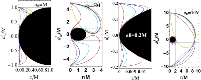
Metric bundles \(\varGamma _{a_0}\) with equal origins \(a_0\), different planes \(\sigma \) and different frequencies \(\omega _b={1}/a_0\sin (\theta )\). The black region is the BH \(a<a_{\pm }\) on the extended plane, gray region is the ergoregion. There \(\theta =\pi /2\) (yellow curve), \(\theta =\pi /12\) (cyan curve), \(\theta =\pi /4\) (pink curve), \(\theta = 2.2 \pi \) (blue curve), \(\theta =3.82\pi \) (red curve). These results follow from the analysis of Eq. (20)
Note that the definition \(r_g(\omega ^M_0)\) holds for the maximum origin, while \(\omega _b(a_0^M)\) is obviously the frequency of the bundle with origin \(a_0^M\); consequently, it holds at each point of the bundle particularly at the tangency point and its origin located at \(a_0\).
The tangent spin has a maximum for \(\sigma \) and for \(a_0\) at \(\sigma ={4}/{a_0^2}\) where \(a_0=M\). However, according to Eq. (10), the tangent point to the horizon is bounded in the range \(r_{g}(\theta )\in [0,r_{g}^*]\in [0,2M]\), where \(r_{g}^*=\left. r_{g}^*\right| _{\theta =\pi /2}={2}/{{4}/({a_0^2})+1}\). The bundle frequency and its tangent point are fixed points under variations of the plane in \(\sigma \in [0,1]\).
We now consider some special cases of metric bundles with equal tangent spin \(a_g\) or radius \(r_g\) or plane \(\sigma \). Some of these cases will be detailed below in dedicated paragraphs, in which we consider two bundles with \((a_0, \sigma , a_g, \omega _b)\) and \((a_0, \sigma _p,a_g^p,\omega _b^p)\), respectively.
$$\begin{aligned}&\mathbf{Metric\,bundles\,with\,equal }\, a_0\mathbf{ and }\,a_g \quad (a_g=a_g^p): \\&\hbox {In this case}\nonumber \\&\bullet \quad a_0\in ]0, 2M[,\quad \hbox {for}\quad \sigma _p\in [0, 1]\quad \hbox {and}\quad \sigma =\sigma _p\nonumber \\&\bullet \quad a_0>2M\quad \mathbf{(i) }\quad \sigma _p\in \left[ 0,\frac{16}{a_0^4}\right. \left[ ,\quad \hbox {and}\quad \sigma =\sigma _p\right. \nonumber \\&\quad \mathbf{(ii) }\quad \sigma _p\in \left[ \frac{16}{a_0^4},\frac{4}{a_0^2} \left. \left. \left[ ,\quad \hbox {and}\quad \sigma \in (\sigma _p,\sigma ^p_{\ell }); \right. \right. \right. \right. \nonumber \\&\left. \left. \mathbf{(iii) }\quad \sigma _p=\frac{4}{a_0^2}\quad \hbox {and}\quad \sigma =\sigma _p,\right. \right. \nonumber \\&\quad \mathbf{(iv) }\left. \left. \quad \sigma _p\in \right] \frac{4}{a_0^2}, 1\right] \quad \hbox {and}\quad \sigma \in (\sigma _p,\sigma ^p_{\ell }) \nonumber \\&\hbox {where}\quad \sigma ^p_{\ell }\equiv \frac{16}{a_0^4 \sigma _p},\quad \hbox {frequency ratio}\nonumber \\&\quad s=\frac{\omega _b}{\omega _b^p}\in \left\{ 1,\frac{\sqrt{\sigma _p}}{\sqrt{\sigma }}=\frac{4}{a_0^2 \sigma }=\frac{a_0^2 \sigma _p}{4}\right\} \\&\mathbf{Metric\,bundles\,with\,equal }\, a_0\,\mathbf{ and }\,\sigma :\nonumber \\&\quad \hbox {In this case} \quad a_g=a_g^p\quad \hbox {and} \quad \omega _b=\omega _b^p \nonumber \\&\mathbf{Metric\,bundles\,with\,equal }\,a_0\,\mathbf{and} \,r_g (\omega _b):\nonumber \\&\quad \hbox {In this case} \quad \sigma =\sigma _p \quad \hbox {and } \quad a_g=a_g^p \nonumber \\&\mathbf{Metric\,bundles\,with\,equal }a_0\,\mathbf{ and }\,a_g\,\mathbf{ and }\,r_g (\omega _b):\nonumber \\&\quad \hbox {In this case} \quad \sigma =\sigma _p.\nonumber \end{aligned}$$(21)Fig. 7 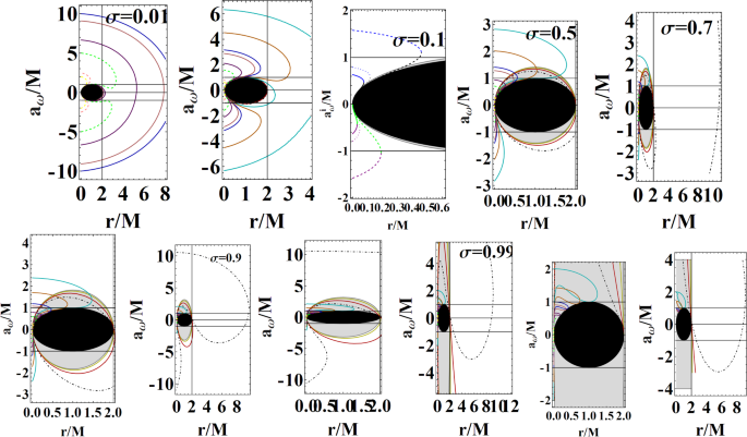
Metric bundles \(\varGamma _{\sigma }\) for the same plane \(\sigma \) and different bundle frequencies \(\omega _b\in \{0.01\) (yellow), 1/27 (Red), 0.1 (dotted-dashed), 0.5 (cyan), 0.7 (orange), 1 (blue), 1.1 (pink), 1.5 (purple), 2 (green), 4 (dashed-pink), 5 (yellow-dashed)}. The black region represents a BH (\(a<a_{\pm }\)) on the extended plane. It follows the analysis of Eq. (23)
Metric bundles with equal \(a_0\) and \(\sigma \), or equal origin and tangent radius \(r_g\) (or frequency) are equal. In the case of equal origin and tangent spin \(a_g\), except for the trivial case of coincidence of the bundle \(\sigma =\sigma _p\), it is noteworthy that only two distinct bundles can exist for NS origins with spin \(a_0>2M\) and large plane \(\sigma _p>{4}/{a_0^2}\), with a fixed ratio between the \(\sigma \) planes and the frequencies. In Sect. 3.2, we will particularly focus on the relations between the frequencies, which are the horizon frequencies \(\omega _H^{\pm }\) (see also Fig. 25). Note that the ratio in Eq. (22) depends on the spin because it is parameterized by the bundle origin \(a_0\), which is related to the bundle frequency through \(\sigma \).
-
Metric bundles \(\varGamma _{\sigma }\) on the same plane \(\theta \) We focus on metric bundles on an equal plane \(\sigma \). The case \(\sigma =1\) has been analyzed in detail in [1]. We will also take into account the results given in Eq. (20). However, we present here some of the relations (20) as follows:
$$\begin{aligned}&\mathbf{Tangent\,radius }\quad r_g(\omega _b)=\frac{2}{4 \omega _b^2+1},\nonumber \\&r_g(a_0)=\frac{2}{\frac{4}{a_0^2 \sigma }+1}, \end{aligned}$$(22)$$\begin{aligned}&\mathbf{Tangent}\,spin \quad a_g(\omega _b)=4 \sqrt{\frac{\omega _b^2}{\left( 4 \omega _b^2+1\right) ^2}},\nonumber \\&a_g(a_0)=\frac{4 a_0\sqrt{\sigma }}{a_0^2 \sigma +4}, \end{aligned}$$(23)$$\begin{aligned}&\mathbf{Bundle\,origin }\quad a_0(\omega _b)=\frac{1}{\sqrt{\sigma } \omega _b},\nonumber \\&\quad a_0(r_g)=\frac{2 \sqrt{r_g}}{\sqrt{2 \sigma -r_g \sigma }}, \end{aligned}$$(24)$$\begin{aligned}&\hbox {where}\quad r_g\in [0,2M],\quad a_0\in [0,+\infty [\cup ]-\infty ,0],\nonumber \\&a_g\in [0,M]\quad \omega _b=\omega _H^{\pm }\in ]0,+\infty [ \end{aligned}$$(25)See the Figs. 1, 4, 5 and 7, where \((r_g(\omega _b)\) and \(r_g(a_0))\) is the tangent radius as function of the bundle frequency \(\omega _b\) and of the bundle origin spin \(a_0\), respectively. The radius \(r_g(a_0)\) is maximum (for \(\sigma \) and \(a_0\)) at \(a_0=\sigma =0\), where \(r_g=2M\). \((a_g(\omega _b),a_g(a_0))\) is the tangent spin as function of the bundle frequency \(\omega _b\) and bundle origin spin \(a_0\), respectively. \((a_0(\omega _b),a_0(r_g))\) is the bundle origin spin as function of the bundle frequency \(\omega _b\) and bundle tangent radius \(r_g\), respectively. The function \(a_g(\omega _b)\) has an extremum at \(\omega _b=1/2\), where \(a_g(\omega _b)=1\).
-
Metric bundles \(\varGamma _{\omega _b}\) with equal bundle frequencies \(\omega _b\)
According to Eq. (23), metric bundles characterized by the same frequency \(\omega _b\) have the same point of tangency with horizon \(r_g\) and tangent spin \(a_g\), but different origin spins \(a_0(\omega _b,\theta )\) for different planes \(\theta \). The relation between the origins of the equal-frequency bundles \(\omega _b\) and, therefore, also the same point of tangency \((a_g,r_p)\), is
$$\begin{aligned}&\mathbf{bundles\, with\, equal } \quad \omega _\mathbf {b} \quad (\mathbf {r}_\mathbf {g},\mathbf {a}_\mathbf {g})\quad \frac{a_0^p}{a_0}=\sqrt{\frac{\sigma }{\sigma _p}}, \end{aligned}$$(26)$$\begin{aligned}&\hbox {in particular}\quad {a_0^p}={a_0}\quad \hbox {iff}\quad \sqrt{{\sigma }}=\sqrt{{\sigma _p}} \end{aligned}$$(27)This case is studied in Fig. 8. This confirms that for each plane \(\sigma \) there is one and only one metric bundle associated with the horizon frequency \(\omega _b\) and the pair \((r_g,a_g)\) (recall that the tangent radius \(r_g\) and, therefore, the tangent spin \(a_g\) are determined by the bundle frequency only, while the bundle origin \(a_0\) depends on the plane \(\sigma \)). In addition, on different planes, there may be different bundles all tangent to the point of the horizon with a radius \(r_g\) and frequency \(\omega _b\), but different \(a_0\) for different \(\sigma \), as follows from Eq. (27). This relation implies the following fact: if the origin \(a_0\) corresponds to a BH, (i.e. \(a_0\in [0,M]\)), it is always tangent to the inner horizon (this will be proved explicitly later especially in Sect. 3.2). Then, a bundle with the same frequency as the inner horizon and therefore the same point of tangency can be generated by an origin \(a_0^p\) in NS related to the frequency by \(a_0^p=a_0\sqrt{\sigma /\sigma _p}\) if \(\sqrt{\sigma _p}\le {\mathcal {A}}_0\equiv a_0\sqrt{\sigma }\). If \(\sqrt{\sigma _p}={\mathcal {A}}_0\), then \(a_0^p\) is always tangent to the point of the horizon that corresponds to the extreme BH. Particularly, for the equatorial plane where \(\sigma =1\) and \(a_0^p=a_0/\sqrt{\sigma _p}\), we conclude that for a fixed point of tangency the minimum origin spin occurs always on the equatorial plane; every other bundle has a higher origin. Then, the bundle with origin in \(a_0=M\) on the equatorial plane has other bundles with equal tangent point necessarily located in the NS region with \(a_0^p=1/\sqrt{\sigma _p}\).
-
Metric bundles \(\varGamma _{a_g}\) with equal bundle tangent spin \(a_g\): construction of horizons
We focus on the case of metric bundles with the same tangent spin \(a_g\). This condition allows us to construct the horizons in the extended plane corresponding to a BH with with spin \(a_g\). We recall that if two metric bundles have the same spin tangent \(a_g\), then irrespectively of the plane \(\sigma \) or origin \(a_0\), they can have either (1) the same frequency \(\omega _b\), i.e., they belong to the family \(\varGamma _{\omega _b}\) studied in Eq. (27), or (2) different \(\omega _b^1\); in any case, i holds that \((\omega _b(a_g),\omega _b^1(a_g))=\omega _H^{\pm }(a_g)\), that is, they must both have one of the horizon frequencies with spin BH spin \(a_g\).
To obtain the relation between these bundles, we use Eq. (23). We divide the problem by considering (1) firstly, a fixed spin \(a_g\) with equal \(\sigma \), and then (2) a fixed \(a_g\) with arbitrary \(\sigma \). This case is studied in Fig. 10. For fixed spin tangent \(a_g\), the two tangent radii are obviously \(r_g=r_{\pm }(a_g)=1\pm \sqrt{1-a_g^2}\), which coincide only for extreme BH case \(a_g=M\). As this a notable case, we will analyze it separately. The metric bundles with the same point of contact \(p_g=(a_g,r_g)\) have the same frequency \(\omega _b\), but pertain to different planes \(\sigma \) and origins \(a_0\); the larger origin spin (for fixed frequency) corresponds to the equatorial plane (\(\sigma =1\)). Thus we obtain a family of metric bundles with the same \((a_g,\omega _b,r_g)\), but different \(a_0(\sigma )\) for different \(\sigma \); each \(\sigma \) corresponds to one and only one bundle with \((a_g,\omega _b,r_g)\).
For fixed \(\sigma \), we now consider metric bundles with equal \((a_g,\omega _b)\) which have equal \(r_g\) related by the horizon curve, i.e., \(r_g^\pm =1\pm \sqrt{1-a_g^2}\). The bundle frequencies \((\omega ^1_b,\omega _b)\) and the bundle origins \((a^1_0,a_0)\) are related as follows
$$\begin{aligned}&\mathbf{Metric\,bundles\,with\,equal } (a_g,\sigma ){:}\quad \omega ^1_b=\frac{1}{4\omega _b},\nonumber \\&a_0=\frac{1}{\omega _b\sqrt{\sigma }},\quad a^1_0=\frac{4\omega _b}{\sqrt{\sigma }}=4\omega _b^2 a_0=\frac{4}{a_0\sigma } \nonumber \\&\hbox {from which }\quad a^1_0 a_0=\frac{4}{\sigma },\quad \frac{a^1_0}{a_0}=4\omega _b^2 \end{aligned}$$(28)$$\begin{aligned}&\mathbf{Metric\, bundles\, with\, equal }\,(a_g,\omega _b,r_g){:} \nonumber \\&a_0^c=\frac{1}{\omega _b\sqrt{\sigma }}=\frac{a_0 \sqrt{\sigma }}{\sqrt{\sigma _c}} \end{aligned}$$(29)$$\begin{aligned}&\hbox {from which}\quad \frac{a_0^c}{a_0}= \sqrt{\frac{\sigma }{\sigma _c}}. \end{aligned}$$(30)Fig. 8 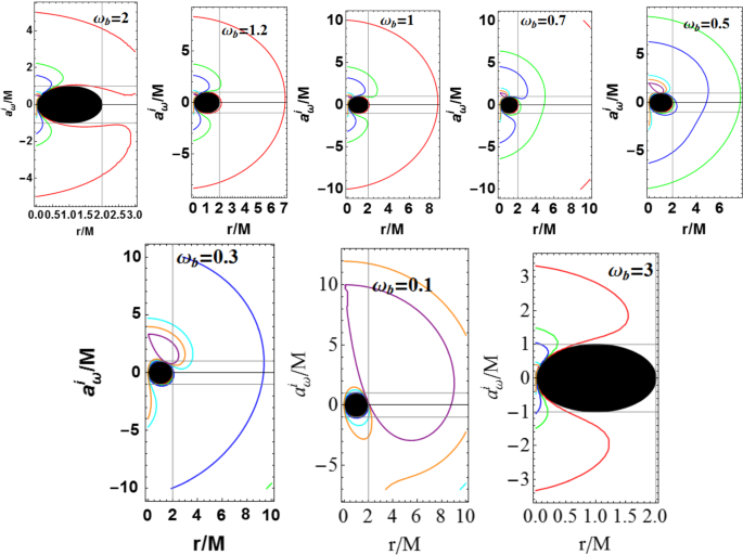
Metric bundles \(\varGamma _{\omega _b}\) with the same frequency \(\omega _b\) and, therefore, also the same spin tangent \(a_g\) and tangent radius \( r_g\). The bundle origins \(a_0\) depend on the plane \(\sigma \): the blue curve is for \(\sigma =0.1\); cyan curve is for \(\sigma =0.5\), green is for \(\sigma =0.05\); orange curve \(\sigma =0.7\), purple curve is \(\sigma =1\), red curve is \(\sigma =0.01\). The black region corresponds to a BH (\(a<a_{\pm }\)) on the extended plane. It follows from the analysis of Eq. (27)
Fig. 9 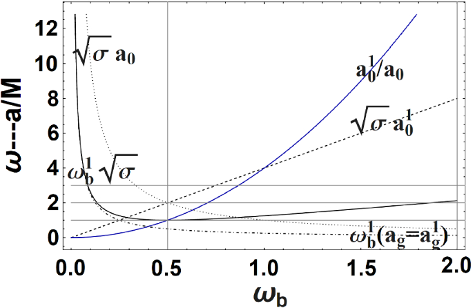
Th black curve is \(\omega _b^1(\omega )\) from Eq. (32), the dashed curve is \(a_0(\omega _b)\sqrt{\sigma }\) for equal \((a_g,\sigma )\) of Eq. (29), the blue curve is \(a_0^1/a_0\) for equal \((a_g,\sigma )\) from Eq. (29), the dotted curve is for \(a_0\sqrt{\sigma }\) for equal \((a_g,\sigma )\) of Eq. (29), the dotted-dashed curve is \(\omega _b^1(\omega _b)\) of Eq. (34) for \(a_{g}(\omega _b^1)=a_{g}^1(\omega _b)\)
Fig. 10 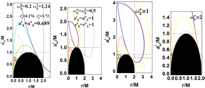
Horizon construction: metric bundles \(\varGamma _{a_g}\) with equal tangent spin \(a_g\) and tangent frequencies \(\omega _g=\omega _b\) and, consequently, equal tangent radius \(r_g\). Construction of horizons \(r_+=r_g^o\) and \(r_-=r_g^i\) for a spacetime with \(a=a_g\) through the corresponding bundle \(a_g^1=a_g^2\) is also shown as the metric bundles with origin \(a_g^i=a_0\). The black region is a BH on the extended plane. Purple and blue curves are for \(\sigma =1\); orange and cyan curves are for \(\sigma =0.97\), darker-yellow and yellow curves are for \(\sigma =0.7\), dotted and dashed curves are for \(\sigma =0.2\), and the red curve is for \(\sigma =1\). It follows from the discussion of Eqs. (29, 32, 34, 35, 37)
The behavior of these quantities is illustrated in Fig. 9.
It is clear that for the class (29), composed by metric bundles with equal \((a_g,\sigma )\), the two bundles have tangent points on the horizon \((r_g,r_g^1)=(r_-(a_g),r_+(a_g))\), generating in this way the horizon of the BH spacetime with spin \(a_g\). We will see also more details below.
-
Corresponding bundles: As studied in [1], there are corresponding bundles with \(a_0^1=a_g\): the tangent point of a bundle is the origin of a second bundle with \(a_0^1=a_g\), which must have a BH origin. Then, we can identify an entire class of corresponding bundles \(\varGamma _{a_g}\) with the same tangent spin, studied in Eq. (29), and the class \(\varGamma _{a_0^1}\) of metric bundles with the same origin, studied in Eq. (20). The frequencies of these bundles are related by
$$\begin{aligned}&\mathbf{Frequency\,relations\,for\,corresponding\, bundles }\nonumber \\&a_0^1=a_g\!: \end{aligned}$$(31)$$\begin{aligned}&\omega _b^p=\frac{4\omega _b^2+1}{4 \sqrt{\sigma {\omega _b^2}}} \end{aligned}$$(32)See Fig. 9. There is an extremum at \(\omega _b^p={1}/{\sqrt{\sigma }}\) for \(\omega _b=1/2\). In general, the following relations hold:
$$\begin{aligned}&\mathbf{Corresponding\,metric\,bundles }\, a_0^1=a_g\!: \nonumber \\&\hbox {It holds}\quad a_{g}(\omega _b^1)=a_{g}^1(\omega _b), \quad \hbox {for}\quad \omega _b^1=\pm \frac{1}{4 (\omega _b)}. \nonumber \\&\hbox {It holds}\quad a_{g}(a_0^1)=a_{g}(a_0), \quad \hbox {and}\quad \sigma =\sigma _1 \nonumber \\&\hbox {for} \quad a_0=\frac{4}{a_0^1 \sigma } \nonumber \\&\hbox { and }\quad \sigma \ne \sigma _1\quad \hbox { for }\quad a_0= \frac{4}{a_0^1 \sqrt{\sigma \sigma _1}}\nonumber \\&\quad \hbox {and}\quad a_0=\frac{a_0^1 \sqrt{\sigma _1}}{\sqrt{\sigma }}. \nonumber \\&\hbox {It holds }\quad a_{g}(a_0,\sigma )=a_{g}^1(a_0,\sigma _1)\quad \hbox {for}\quad \sigma _1= \frac{16}{a_0^4 \sigma }.\nonumber \\ \end{aligned}$$(33)See Fig. 9. The tangent radii for these bundles are
$$\begin{aligned}&\mathbf{Tangent\,radii }\quad r_g(\omega _b)=r_\flat \quad \hbox {for}\quad a=\sharp \frac{4 \omega _b}{4 \omega _b^2+1},\nonumber \\&\hbox {where}\quad \flat =\pm ,\quad \sharp =\pm , \end{aligned}$$(34)$$\begin{aligned}&r_g(\omega _b)=r_g(\omega ^p_b)\quad \hbox {for}\quad \omega ^p_b=\pm \omega _b;\quad r_g(a_0)=r_\flat \nonumber \\&\hbox {for}\quad a=\sharp \frac{4a_0 \sqrt{\sigma }}{a_0^2 \sigma +4}, \nonumber \\&r_g(a_0^1,\sigma ^1)=r_g(a_0,\sigma )\quad \hbox {for}\quad a_0^1=\pm \frac{a_0\sqrt{\sigma }}{\sqrt{\sigma _1}} \end{aligned}$$(35)(the use of \(\flat \) and \(\sharp \) for the sign convention means that there is no correspondence between the two options). The following special points determine some particular values of the bundles:
$$\begin{aligned}&\hbox {}\quad a_g=M\quad \hbox {for}\quad \omega _b=\pm \frac{1}{2},\quad a_g=M\nonumber \\&\hbox {for}\quad a_0^2 = \frac{4}{\sigma },\quad \hbox {and}\quad a_g(a_0=M)=\frac{4 \sqrt{\sigma }}{\sigma +4},\nonumber \\&\quad a_g(0)=0. \nonumber \\&r_g=M\quad \hbox {for}\quad \omega _b=\pm \frac{1}{2},\quad \hbox { and}\quad r_g(a_0)=M\quad \nonumber \\&a_0 = \frac{2}{\sqrt{\sigma }}. \nonumber \\&\hbox {For}\quad a_0=M \quad \hbox {it holds}\quad \omega \rightarrow \frac{1}{\sqrt{\sigma }} \end{aligned}$$(36)$$\begin{aligned}&\lim _{a_0\rightarrow +\infty }a_g= \lim _{a_0\rightarrow +0}a_g= \lim _{a_0\rightarrow +\infty }\omega _b=0, \nonumber \\&\lim _{a_0\rightarrow +0}\omega _b=\infty ,\quad \lim _{a_0\rightarrow +0}r_g=0,\quad \lim _{a_0\rightarrow +\infty }r_g=2M,\nonumber \\&\hbox {and}\quad r_g=2M \quad \hbox {for}\quad \omega _b=0, \end{aligned}$$(37)see Fig. 10. These limiting frequencies will be found also in the frequency relations of Sect. 3.2.
-
On the relation between origin spin and tangent spin
Consider the origin frequency \(\omega _0\), associated with a spacetime with origin spin coincident with the tangent spin (\(a_0=a_g\)) of a bundle with frequency \(\omega ^p_b\), plane \(\sigma _p\) and origin \(a_0^p\), there is then
$$\begin{aligned}&\hbox {for}\quad \sigma =\sigma _p\quad \omega _0^{\pm }(a_g)=\frac{1}{a^p_0 \sigma }+\frac{a^p_0}{4}, \end{aligned}$$(38)$$\begin{aligned}&\omega _0^{\pm }(a_g)=\frac{4 (\omega ^p_b)^2+1}{4 \sqrt{\sigma } \omega ^p_b},\quad \hbox {where}\quad a_g=a_g(a_0^p) \nonumber \\&\sigma \ne \sigma _p\quad \omega _0^{\pm }(a_g)=\frac{a_0^p}{4} \sqrt{\frac{\sigma _p}{\sigma }}+\frac{1}{a_0^p \sqrt{\sigma \sigma _p}}, \end{aligned}$$(39)where the tangent spin of the bundle with origin in \(a_g\) is
$$\begin{aligned}&a_g^p=\frac{4 a_0^p \sqrt{\sigma \sigma _p} \left[ (a_0^p)^2 \sigma _p+4\right] }{(a_0^p)^2 \sigma _p \left[ (a_0^p)^2 \sigma _p+4 \sigma +8\right] +16}.\quad \end{aligned}$$(40)In this way, we also obtained a relation between the origins \((a_0,a_0^p)\) and the characteristic frequencies of the two corresponding MBs. The relation between the frequencies \((\omega _b,\omega _b^p\)) is clearly independent of the plane \(\sigma _p\), because it is included in the form of \(\omega _b^p\) in terms of the origin spin. The tangent spin \(a_g^p\) has a maximum in terms of the first MB origin as \(a_0\) as \(\sigma _p={4}/{(a_0^p)^2}\) – see Fig. 11.


Analysis of Eq. (39). Upper panel: for \(\sigma =1\), \(a_g^p\) of the corresponding bundle (cyan), origin of the corresponding MBs (cyan, dashed), frequency \((1/a_0^p)\) (orange), frequency of the corresponding MBs (orange dashed), origin \(a_0^p\) (black) as function of \(a_0^p\). The below panel illustrates the frequencies relations \(\omega _b^p\) as functions of the bundle frequencies of Eq. (39) for different planes \(\sigma \). The orange line is the \(\omega _b=\omega _b^p\)
2.6.2 Crossing of metric bundles: determination of the orbital limiting frequencies
Metric bundles cross on the extended plane at a point (a, r). The two frequencies \((\omega _1, \omega _2)\) of a MB with fixed \((a,\sigma ,r)\) are related as
where \(\omega _1\) and \(\omega _2\) are given as \(\omega _{\pm }\) in Eq. (8). The two origins of the MBs, as functions of any point in the bundle \((r,a,\sigma )\), are
Conditions (44) show MBs solutions with the same origin \(a_0\) and tangent point in \((a,r,\sigma )\), that is, the same spin a, equal plane \(\sigma \) and crossing radius r. This analysis is related to the horizon curve, where
Obviously, the second frequency at a point of the bundle geometry is also a horizon frequency, that is, if \(\omega _b\) is a bundle frequency, then at the point r a photon will have orbital frequency \(\omega _b\), while the second frequency of the couple \(\omega _{\pm }\) is associated with the horizon frequency of the bundle crossing at the point (a, r).
If \((a_{\times },r_{\times })\) represent the crossing points of two MBs with frequencies \(\omega _b(a_g)<\omega ^p_b(a^p_g)\), it is clear that \(\omega _b(a_g)=\omega _H^{+}(a_g)\) and \(\omega ^p_b(a^p_g)=\omega ^-_H(a^p_g)\). It follows that the two crossing MBs are necessarily one tangent to an outer horizon and another one tangent to an inner horizon. On the other hand, the relation between MBs frequencies is independent of the angle \(\theta \) (equivalently \(\sigma \)) as the bundle characteristic frequencies are horizon frequencies (they will, of course, depend on the plane \(\sigma \) when related to their bundle origin spins). Now, it is possible to find MBs crossing at a point \((r_{\times },a_{\times })\) of the extended plane, which have different planes \(\sigma \). However, such MBs relate, in the geometry with crossing spin \(a_{\times }\), frequencies associated with the crossing orbit \(r_{\times }\), but on different planes \((\sigma ,\sigma _p)\) of the same Kerr geometry. It is possible to constraint this case considering \(\omega _{\pm }\) in Eq. (8) as functions of \(\sigma \) only or, viceversa, using the solutions \(\sigma _{\omega }^{\pm }\) of Eq. (120) as functions of \(\omega \).
However, we note that for fixed \(\sigma \) at the point \((a_{\times },r_{\times })\) there are frequencies \((\omega _H^{+}(a_g),\omega _H^{-}(a_g^p))\) for two tangent bundle spins \((a_g,a_g^p)\), respectively. Because of the existence of the two frequencies \(\omega _{\pm }\) per point per spin and per plane, we infer that at each point of the extended plane there is an even number of crossing MBs (a part of the limiting case of the horizon curve). In particular, for the same plane \(\sigma \), we have that
and the relations (23) hold as special cases of \(\varGamma _{\sigma }\). In general, the following relations hold:
In Fig. 12, we show the frequencies at a fixed point (a, r) of the extended plane for different \(\sigma \). Notice the frequency signs (negative for retrograde photon motion) and the decreasing behavior of the frequencies in terms of the plane \(\sigma \) at fixed r. Notice also the role of the ergoregion. In the next Section, we will focus particularly on MBs with fixed a and characteristic frequency equal to \(\omega _H^{\pm }(a)\). This is clearly the problem of the MBs confinement with a frequency equal to the horizon frequency.

Upper lines: bundle frequencies \(\omega _{\pm }\) as functions of the plane \(\sigma \in [0,1]\) for fixed spin a/M and radius r/M of the extended plane. Note the frequencies signs (negative for retrograde photon motion)) and the decreasing magnitude with the plane \(\sigma \) at fixed r. The limiting roles of the horizons and ergosurfaces can also be noted. Below lines: solutions \(\omega _{\pm }\)=constant on the \((r/M,\sigma )\) plane. Note the frequencies sign, always positive in the ergoregion (red curves are the ergosurfaces \(r_{\epsilon }^{\pm }\)), horizons are also show. The curves are studied for different spins \(a/M>0\). See the analysis of Sect. 2 on the crossing of metric bundles and determination of orbital limiting frequencies
3 Extracting information from Kerr metric bundles: Photon frequency and horizon frequencies
We now consider the condition \(\omega _x=\omega _y\), where \(\omega _x\in \{\omega _+,\omega _-\}\) and \(\omega _y\in \{\omega _H^-,\omega _H^-\}\). We look for all those solutions of \({\mathcal {L}}_{{\mathcal {N}}}\equiv {\mathcal {L}}\cdot {\mathcal {L}}=0\) associated to orbits r different from the horizon, but characterized by a photon with orbital frequency equal to that of the horizon per equal a. We are looking for solutions of the normalization condition \({\mathcal {L}}_{{\mathcal {N}}}=0\) when \(\omega =\omega _H(a)\) for a geometry with spin a with a \({\bar{r}}\ne r_{\pm }\). We are particularly interested in cases where \({\bar{r}}>r_+\), from which the most relevant case is for \({\bar{r}}>r_+\) with \(\omega _{*}({\bar{r}})=\omega _H^-\) for \(\omega _{*}\in \{\omega _+,\omega _-\}\).
Combining the considerations of the bundle crossing and inner horizon confinement problem, we note that the existence of an “external” orbit (at \(r>r_+\)), with one frequency equal to the inner horizon frequency on the extended plane, implies that in the region \(r>r_+\) bundles tangent to the inner and outer horizons intersect. We are then confronted with a two-sided problem: 1. The problem of finding a point \(r>r_+({\bar{a}})\) in \({\bar{a}}\in [0,M]\) with frequency \(\omega _H^-(a_*)\) for a general spin \(a_*\ne {\bar{a}}\) such that \(\omega _\pm ({\bar{a}})=\omega _H^-(a_*)\). 2. The problem of finding a solution \(\omega _\pm ({\bar{a}})=\omega _H^-({\bar{a}})\) (i.e. \(a_*= {\bar{a}}\)). We have met this kind of problems in several parts of our investigation. We will show that the second problem exists on planes very close to the rotation axis. Consider the spin \({\bar{a}}=\)constant of a bundle with frequency \(\omega _H^-({\bar{a}})\) on a plane \(\sigma \) and analyze the problem for \(\sigma \) with \(r>r_+({\bar{a}})\) and \(\omega _{\pm }({\bar{a}})=\omega _H^-({\bar{a}})\). It can be proved that solutions of this problem are \(r_{\pounds }\) (or, equivalently, in terms of the spin \(a_{\pounds }\) and in terms of the plane \(\sigma _{\pounds }\)), if the following conditions are satisfied

Inner horizon confinement on the extended plane. Constraints on the existence of orbits of the exterior region on the extended plane \(r>r_+\) with frequencies \(\omega _-=\omega _H^-\). See the analysis of Sect. 3 and Eq. (47). Left panel: orbits \(r_{\pounds }\) solutions of \(\omega _-=\omega _H^-\) (photons defined by the condition \({\mathcal {L}}_{{\mathcal {N}}}=0\)) as function of the plane \(\sigma \in [0,1]\) for different spins a/M. The limiting value \(a=M\), black curve coincident also with \(r_{descr}(\sigma )\). The solutions of \(\omega _-=\omega _H^-\) clearly include also the inner horizon \(r_-(a)\). The horizons \(r_{\pm }(a)\) are also showed (horizontal lines). The limiting value \(\sigma _{descr}\approx 0.53M\). A solution is clearly the inner horizon \(r_-\). The larger is the BH spin, the larger can be the plane value function \(\sigma \le \sigma _{decr}\). Shaded regions are confinement regions. Below: 3D plot is \(r_{\pounds }\), containing a solution of \(\omega _-=\omega _H^-\) as function of a/M and \(\sigma \). Quantities are defined in Eqs. (52, 49, 50, 51)
and \(\sigma _{\pounds }\), \(a_{\pounds }\) and \(r_{\pounds }\) are solutions of the equations
respectively, whereas the limiting spin \(a_{\delta }\) is a solution of the following equation
We show the behavior of these quantities and the constraints for the existence of orbits with frequency of the inner horizon in the outer region of the extended plane \(a>a_+\) in Fig. 13.
A more detailed study of the frequency ratio of MBs as horizon frequencies is given in Sect. 3.2.
As we shall see in detail also in Sect. 3.2, bundles with origin spin in the weak black holes (WBH) region of the extended plane, i.e., with \({\mathcal {A}}_0=a_0\sqrt{\sigma }\le 4/5\le 0.8M\), for sufficiently large values \(\sigma \lessapprox 1\) and particularly on the equatorial plane, are entirely confined in the BH region (the inner region of the extended plane as in Fig. 2). It follows that their characteristic frequencies (with tangent spin \(r_g\in ]0,2M/5[\) and characteristic frequencies \(\omega _b\ge 1\))) can never be “replicated” in those planes in the outer region of the extended plane. However, constraints can be found in terms of the variable \({\mathcal {A}}_0\). Frequencies \(\omega _b\ge 0.5\) (range of \(\omega _H^-\)) for orbits in the outer region are shown in Figs. 6, 7, 8, 10, 14 and 15.

Frequencies \(\omega _{\pm }\) for different spins a/M and planes \(\sigma \), as functions of r/M. The horizontal lines are horizon frequencies \(\omega _H^{\pm }\), vertical lines are the inner and outer horizons \(r_{\pm }\). There are solutions \(\omega =\omega _H^{\pm }\) particularly for \(r>r_+\), according to Eqs. (59, 60)

Horizon frequency solutions of the MBs in the exterior region are horizontal lines of the extended plane in Fig. 2. The plots show, for fixed plane \(\sigma \equiv (\sin \theta )^2\), the inner and outer horizons, the inner and outer ergosurfaces, the circle in the outer horizon, (red) on the inner horizon (blue) and orbital solutions with frequency of the inner (blue) and outer (red) horizon. In the frame we use, the BH Kerr ring singularity is at \(r=0\). In the lower panels, the light surface solutions \(\{r_s^1,r_s^2,r_s^4\}\) of Eq. (116) are plotted for \(\omega =\omega ^+_H\) (orange) in \(\omega =\omega ^-_H\) (darker cyan). Black curves are the inner and outer ergosurfaces and the inner and outer Killing horizons. These orbits contain replicas of the horizons as defined in Eq. (138)
This is a consequence of the fact that if the \((a_g, r_g)\) relations can be expressed as functions of \({\mathcal {A}}=a\sqrt{\sigma }\), this does not hold for the quantity \({\mathcal {L}}_{{\mathcal {N}}}\); consequently, it follows that the bundles can extract “information” on the inner horizons frequencies near the rotation axis and, therefore, in this sense, the inner region is not entirely confined. Equally, MBs with weak naked singularities (WNS) origins, i. e., with \({\mathcal {A}}_0=a_0\sqrt{\sigma }\in ]M,2M]\), which complete the inner horizon with tangency radius \(r_g\in ]2M/5,M[\), spin \(a_g\in ]0.8M,M]\) and characteristic frequency \(\omega _b\in [0.5,1[\)), for small \(\sigma \) can be found in the outer region of the extended plane. We shall see this in details in Sect. 3.2.
For the equatorial plane, \(\sigma =1\), this condition was considered in detail in [1], where the concept of inner horizon confinement was introduced. We resume this issue as follows (see Fig. 14). It was shown that there are two radii \(r_\pm ^\pm \) such that \(r_-^-<r_-<r_+<r_+^+\) almost everywhere (exceptions are at \(a_g=0\) and \(a_g=M\)) and \(\omega _*(r_\pm ^\pm )=\omega _H^\pm \), respectively.
The problem of finding solutions of \({\mathcal {L}}_{{\mathcal {N}}}=0\) for \(\omega _H^{\pm }\) is clearly related to the characterization of the MBs \(\varGamma _{a_g,\omega _b}\), constituted by the MBs \(\varGamma _{a_g}\) with equal tangent spin \(a_g\) and already analyzed in Eq. (29), and equal frequency \(\varGamma _{\omega _b}\) (and equal tangent radius \(r_g\)) also analyzed in Eq. (27). Therefore, the particular relations given in Eq. (30) are valid.
There are then two classes of MBs to be considered. Firstly, we focus on equal \(\sigma \) solutions, discussed in Eq. (30). Solutions \(r: \omega _{\pm }(r)=\omega _H^{\pm }(a_g)\) belong to the same bundle and, therefore, depend on the bundle curves bending (curvature) on the extended plane. In fact, as follows from Figs. 6, 7, 8 and 10, the situation is simple in the case \(\sigma =1\), where there are two bundle branches (closed on the horizons) corresponding to the two solutions \(r_{\pm }^{\pm }\), respectively. Alternatively, the analysis can be performed by considering the frequency solutions (8) directly (see Fig. 14, where the horizon-frequency solutions are given by horizontal lines (corresponding to \(\omega =\omega _H^{\pm }\)) on the extended plane.
Solutions for equal planes and equal tangent frequencies belong to the same metric bundle; therefore, they must share the same origin \(a_0\). (The relevance of the equatorial case \(\sigma =1\) for the Kerr MBs analysis lies also in the fact that for the spherically symmetric, static and electrically charged Reissner Nortström solution, the MBs curvature properties in the extended plane are similar to the off-equatorial case of the Kerr geometry, showing the interplay between symmetries and geometry in defining the MBs properties – [1].) Then, for a general \(\sigma \), we consider the two-faced problem for the orbits of frequencies \(\omega _H^{\pm }\), considering the MBs \(\varGamma _{a_g}^-\equiv \{g_{\omega }(a_g,r_g^-)\}_{\sigma }\) and \(\varGamma _{a_g}^+\equiv \{g_{\omega }(a_g,r_g^+)\}_{\sigma }\), where \(r_{g}^{\pm }\) are, respectively, the tangent points of the two bundle families on the outer and inner horizons of the BH with spin \(a_g\). To these MBs correspond, respectively, the horizon frequencies \(\omega _b^->\omega _b^+\) of the BH spacetime with spin \(a=a_g\). In the second case, we consider in the classes \(\varGamma _{a_g}^\pm \) the pairs \((g_{\omega }(a_g,r_g^-,\sigma ),g_{\omega }(a_g,r_g^+,\sigma )) \in \varGamma _{a_g,\sigma }^-\times \varGamma _{a_g,\sigma }^+\) i.e. with the same \(a_g\) on the same \(\sigma \) (recall that the horizon frequencies \(\omega _b^{\pm }\) are independent of \(\sigma \), a property linked to the BHs horizon rigidity).
We now focus on the range \(a\in [-M,M]\) of BH spacetimes. In fact, for different a, solutions are provided as MBs intersections which, for each plane \(\sigma \) at each point r (except for the origin), involve only two bundles. This case is considered in Fig. 16, where we see solutions for \(r\ne r_{\pm }\) for small values of \(\sigma \) and for \(r_-^o>r_+\) with frequencies \(\omega _{H}^-\), that is, equal to the frequency of the inner horizon which, therefore, is not confined to \(r<r_-\).

Photon orbital frequencies and horizon frequencies. In the plane (a/M, r/M), for different planes \(\sigma \), the solutions \(\omega _+=\omega _+(r_-)\) red curve, \(\omega _-=\omega _-(r_-)\) black curve, \(\omega _-=\omega _-(r_+)\) orange curve, \(\omega _+=\omega _+ (r_+)\) purple curve. The black region is a BH on the extended plane \(r\in [r_-,r_+]\), the gray region is the ergoregion
3.1 Replicas construction
To clarify the concept of replicas, in Fig. 18 we show a set of replicas of the inner and outer horizons, providing notes on their constructions in Fig. 17. We consider a BH with spinFootnote 9\(a=a_{\gamma }^{\epsilon }=0.994298M\). We note, on the left panel of Fig. 17, the symmetry around the equatorial plane (\(\theta =\pi /2\) or \(\sigma =1\)) which is clear also from the orbits in Fig. 18. The inner horizon frequencies are confined (in the region \(r<r_-\)) for angles close to the equatorial plane (we also note that the vertical axis as in Fig. 18 is \(z=r\cos \theta =r\sqrt{1-\sigma }\)). Replicas of the inner horizon frequency are also in the outer region \((r>r_+)\) for \(\theta \) far from the equatorial plane. There are two extreme values of \(\theta \) for the existence of the inner horizon replicas in the outer region, where the outer horizon replicas are well defined for any plane. There are replicas inside the outer ergosurface but no replicas are in the region \(]0,r_{\epsilon }^-[\). A further interesting aspect is the asymptotic behavior (for large r/M), where the outer horizon and the inner horizon replicas curves close and approach the BH poles (i.e. \(\theta =\{0,\pi \}\), therefore for larger r and small \(\sigma \)). This means that at fixed angle \(\sigma \), the inner horizon replica approaches the outer horizon replica. Similarly, at fixed radius r/M, there are two replicas for two horizons frequencies respectively, for close values of \(\theta \)s approaching the pole. A study of this asymptotic region is done also in Fig. 17 – the right panel, in terms of the parameter \(\sigma =\sin ^2\theta \). We note that for small \(\sigma \) and large r the two curves, inner and outer horizons replicas, get closer. We also note the presence of the inner horizon confinement for \(\sigma > rsim 0.8\) while there are replicas of the inner horizon in the outer region for \(\sigma \lesssim 0.27\). A replica of the outer horizon for \(\sigma =\sigma _1\) is on the outer ergosurface.

Study of replicas for the BH spacetime with spin \(a_{\gamma }^{\epsilon }=0.994298M\): \(r_{\pm }\) are the outer and inner BH horizon. \(r_{\epsilon }^{\pm }\) are the outer and inner ergosurfaces. \(\omega _H^{\pm }\) are the frequencies of the outer and inner horizon respectively. \(\omega _{\pm }\) are solutions of light like orbital frequencies for stationary observers. There is \(\sigma \equiv \sin ^2\theta \). See Fig. 15 and in Fig. 18. Left panel: vertical lines are the horizons \(r_{\pm }\), the singularity \(r=0\) and the ergosurface \(r_{\epsilon }^+=2M\) on the equatorial plane \(\theta =\pi /2\). and \(r_{\epsilon }^{\pm }\). Yellow curve is the \(r_{\epsilon }^+\), cyan curve is \(r_{\epsilon }^-\). Replicas of light like orbital frequencies \(\omega _+\) black and \(\omega _-\) gray, in the plane \(\theta -r\). Replicas of the frequency \(\omega _H^+\) are the dashed curves, replicas of the frequency \(\omega _H^-\) are the plain curves. Right panel: \(\sigma _1\) and \(\sigma _2\) are selected values of the plane \(\sigma \) whose replicas are showed in Fig. 17. Gray region is the range \(]r_+,r_-[\), gray curves are the radii \(r_{\epsilon }^{\pm }\). Brown curves are the orbits and plane with the inner horizon frequency, the dashed curves are the orbits and plane with the outer horizon frequencies. \(\sigma =1\) is the equatorial plane while \(\sigma =0\) are the BH poles

Examples of horizons replicas are shown for fixed \(\sigma _1=0.50466\) and \(\sigma _2=0.25\), where \(\sigma \equiv \sin ^2\theta \), in a BH geometry with spin \(a_{\gamma }^{\epsilon }\equiv 0.994298M\). The \(\sigma \)s parameters are selected according to the considerations in Fig. 17. Green sphere is the inner BH horizon \(r_-\), blue sphere is the outer BH horizon \(r_+\), light gray surfaces are the inner and outer ergosurfaces \(r_{\epsilon }^{\mp }\). Brown orbits are replicas for \(\sigma =\sigma _1\), purple curves are replicas for \(\sigma =\sigma _2\). Dashed are replicas of the outer horizon, plain curves are replicas of the inner horizons. In upper line panels there are flat coordinates \(\{x=r \sin (\theta ) \cos (\phi ),y=r \sin (\theta ) \sin (\phi ),z=r \cos (\theta )\}\) (central singularity is the point \(r=0\) at \(x=0\), \(y=0\) and \(z=0\)). In below line panels there are the coordinates \(\left\{ x=\sqrt{a^2+r^2} \sin (\theta ) \cos (\phi ),y=\sqrt{a^2+r^2} \sin (\theta ) \sin (\phi ),z=r \cos (\theta )\right\} \), (central singularity is the central disk of radius a). The replicas are the orbits defined by the crossings of the vertical lines \(\sigma _1\) and \(\sigma _2\) of Fig. 17 with the brown curves (inner horizons frequencies) and dashed curves (outer horizons frequencies). Replicas are for \(\sigma = 0.25\), for frequency \( \omega _H^+ : \{r/M=3.0586, r_ + /M = 1.1066, r/M=0.8264\}\), for \( \omega _H^- :\{r/M=1.8267, r/M=1.3361, r_ - /M = 0.893\}\). Replicas for \(\sigma = 0.50466\) are: for \(\omega _H^+ : \{r/M=1.7143, r_ + /M = 1.1066, r/M= 0.6556\}\) for \( \omega _H^-\) there is the only inner horizon \(r_-\)
3.2 Results
We study the problem of finding solutions with a frequency that coincides with that of the inner horizon \(\omega _H^-\). There are two possibilities:
-
1.
There are no solutions of \(\omega _+=\omega _+(r_-)\) for \(r>r_-\) in \(a\in [0,M]\).
-
2.
There are instead solutions of \(\omega _-=\omega _-(r_-)\). In this case, we express the solutions in terms of the plane \(\sigma \):
The behavior of these quantities is illustrated in Figs. 19 and 16.

Photon orbital frequencies as horizons frequencies. Solutions of \(\omega _-=\omega _-(r_-)\) for \(a\in [0,M]\), and of \(\omega _+=\omega _+(r_-)\) for \(a\in [-M,0]\) for \(r>r_-\)–Eqs (59) and (53). Left panel: \(a_{descr}/M\) as function of \(\sigma \equiv \sin ^2\theta \). Center panel: solutions \(\omega _-=\omega _-(r_-)\) on the plane (r/M, a/M) for different planes \(\sigma \in [0,1]\); a zoom for \(a\approx M\) is in the right panel. The black region is a BH on the extended plane (\(r\in [r_-,r_+]\)). Below panel: solutions \(\omega _-=\omega _-(r_-)\) as functions of r/M for \(\sigma \in [0,1]\) and \(a\in [0,M]\). The gray region represents the ergosphere on the extended plane
3.2.1 The discriminant spin \(a_{descr}(\sigma )\)
For the problem under consideration an important quantity is the discriminant spin \(a_{descr}(\sigma )\in [0,M]\), which is a solution of the following equation
The radii r corresponding to frequencies equal to that of the horizon are solutions of the equation
More precisely, there are solutions of the problem \(\omega _-=\omega _-(r_-)\) as follows:
This implies that the occurrence of orbits \(r>r_-\) with photon orbital frequency equal to that of the inner horizon is expected for small \(\sigma \) (\(\sigma \in [0,\sigma _{descr}]\)) and larger spins (\(a\in [a_{descr},M]\)) – Figs. 14, 16 and 19. It should be noted, as evident also from Fig. 14, that \(a_{descr}\approx M\) for \(\sigma \lnapprox M\) and \(\sigma \gnapprox 0\). Finally, the radii \((r_-^-,r_{\diamond },r_{\star }, r_{\circ },{\hat{r}}_-^-,\check{r}_-^-)\) of Eqs. (59) and (60), are solutions of Eq. (58), where \(r_-^-\) is provided in [1].
We now consider negative spins for retrograde orbits, i.e., \(a\in [-M,0]\). There are solutions of \(\omega _+=\omega _+(r_-)\) for \(r>r_-\) similarly to the conditions (59) and (60) in \(a\in [-M,0]\) – Fig. 14. We also address this analysis in more details in Sect. B.1.
There are no solutions of \(\omega _{-}=\omega _{H}^{+}\) for \(r>r_-\).
Moreover, for \(\omega _{+}=\omega _{H}^{+}\), we obtain
Note that the radii \((\hat{{\hat{r}}},{\tilde{r}},\breve{\breve{r}},\tilde{{\tilde{r}}})\) are solutions of Eq. (58), where \(r_+^+\) is given in [1]. For \(a\in [-M,0]\), there exist solutions for \(\omega _{-}=\omega _{H}^{+}\), similarly to the former case (in fact, the equations have some remarkable symmetries). The second frequency at point r is
In Sect. B.3, we complete this analysis by introducing the definition of horizon replicas. We investigate the vertical lines of the extended plane crossing the horizon curve, in other words, the metric bundles with characteristic frequencies
with orbits located exactly in \(r_\pm (a_p)>r_+(a)\), that is, on the horizon with frequency \(\omega _b(a)=\omega _H^\pm (a_p)\).
3.2.2 On retrograde solutions with frequencies equal to the horizon frequencies.
We also investigate photon orbits, solutions of \({\mathcal {L}}\cdot {\mathcal {L}}=0\), with frequencies equal and opposite to the horizon frequencies. Because of the symmetries we can restrict ourselves to the case \(\omega >0\) and \(a\in ]-M,0[\). We recall that the condition \({\mathcal {L}}_{{\mathcal {N}}}=0\) is symmetric under the inversion \(a\rightarrow -a\) and \(\omega \rightarrow -\omega \), i.e. \({\mathcal {L}}_{{\mathcal {N}}}(a,-\omega )={\mathcal {L}}_{{\mathcal {N}}}(-a,\omega )\) and thus \({\mathcal {L}}_{{\mathcal {N}}}(-a,-\omega )={\mathcal {L}}_{{\mathcal {N}}}(a,\omega )\). Our analysis is not focused on the retrograde case (negative frequencies); however, this case is relevant because the corresponding frequencies are equal in magnitude to the horizon frequencies. A systematic analysis of this case is considered in Sect. B.1.
3.3 Horizon frequencies as bundle frequencies
The fact that the bundle frequency \(\omega _b\) coincides with the horizon frequencies \(\omega _H^{\pm }(a_g)\) with spin \(a_g\) and, consequently, each photon orbital frequency, \(\omega _+(a)\) or \(\omega _-(a)\), at any point \((r,a,\sigma )\) and any azimuthal angle \(\varphi =\)constant in any geometry a of the bundle \(a_{\omega }^{\pm }\) is a horizon frequency in the extended plane, allows us to analyze the bundle properties and, therefore, the Kerr spacetime causal structure in terms of horizon frequencies.Footnote 10
This analysis also allows us to better understand the MBs meaning and specifically the relations between the origin \(a_0\) and the bundle tangent spin \(a_g\) as given in Eqs. (11) and (17). The relation \(a_g(a_0)\) given in Eq. (11), as function of \({\mathcal {A}}\equiv a \sqrt{\sigma }\), is similar to that of the case \(\sigma =1\) as follows from Fig. 5. Consequently, all the results concerning \((a_g,r_g,\omega _b)\) obtained for the equatorial case are valid also for \(\sigma \in ]0,1[\), in terms of \({\mathcal {A}}\equiv a \sqrt{\sigma }\); see Eq. (17) and Fig. 5.
In [1], we demonstrated that for \(\sigma =1\):
\(\bullet \) MBs with BH origins \(a_0\in [0,M]\) are all tangent to the inner horizon and, therefore, have tangent spin \(a_g\in [0,0.8M]\) and tangent radius \(r_g\in [0,2/5M]\) with frequencies \(\omega _b=\omega _H^-\ge 1\) – see Fig. 23. These MBs are all confined in the region of the extended plane upper-bounded by the inner horizon (because \(a_0\ge a\ge a_g\) for any spin a of the bundle)–(see the \(\mathbf {BB}\) model of [1]).
\(\bullet \) MBs with WNS origins \(a_0\in [M,2M]\) can be used to construct only a portion of the inner horizon with \(a_g\in [0.8M,M]\), \(r_g\in [2/5M,M]\), and \(\omega _b\in [0.5,1[\). These bundles are made of NSs and BHs.
\(\bullet \) Metric bundles with strong naked singularities origins (SNSs), \(a_0> 2M\), can be used to construct only the outer horizon on the extended plane.
These results have some remarkable implications:
-
1.
On the equatorial plane and, more generally, for sufficiently large values of \(\sigma \in [0,1]\), MBs with BH origins are all confined in the inner region of the extended plane (bundles confinement) – see Fig. 2. Consequently:
-
2.
All the frequencies \(\omega _b\ge 1\) belonging to these bundles cannot be found in the NS regime nor in the outer region (\(r>r_+\)) on the extended plane for large values of \(\sigma \) (frequencies confinement). Results (1) and (2), therefore, hold if we consider the variable \({\mathcal {A}}_0=a_0\sqrt{\sigma }\).
-
3.
The bottleneck region of Fig. 2, including NS metric bundle origins \({\mathcal {A}}_0\equiv a_0\sqrt{\sigma }\in [M,2M]\), with bundle characteristic frequencies \(\omega _b\in [0.5,1[\) remain confined to the BH inner region or to the NS region, i.e., they are outside the region \(r>r_+\) and \(a\in [0,M]\), for large values of \(\sigma \).
-
4.
All MBs with an origin spin of a NS have characteristic frequencies of the outer horizon on the extended plane, apart from the bottleneck region (\({\mathcal {A}}_0\in [M,2M]\)), where MBs have the frequencies of the inner horizon. We can see this relation, in terms of \({\mathcal {A}}\) between tangent spin and tangent radius also in Fig. 21. As it is clear from the analysis of Sect. 3.2, there are bundles (and therefore orbits) with characteristic frequencies equal to the outer horizon frequencies, which are located in the inner region of the extended plane. Vice versa, outer horizon frequencies and are all and only those of NS origins \({\mathcal {A}}_0=a_0\sqrt{\sigma }\ge 2M\) for any plane \(\sigma \) (thus, \(a_0\ge 2M/\sqrt{\sigma }\ge 2M\)).
The results (4) imply that the outer horizon can be constructed only by strong naked singularity origins with \({\mathcal {A}}_0\ge 2M\) and, therefore, with \(a_0\ge 2M/\sqrt{\sigma }\ge 2M\).
More precisely, concerning the inner horizon confinement, as the relations \(a_g(a_0,\sigma )\), \(r_g(a_0,\sigma )\) and \(\omega _b(a_0,\sigma )\) can be read as \(a_g({\mathcal {A}}_0)\), \(r_g({\mathcal {A}}_0)\) and \(\omega _b({\mathcal {A}}_0)\), then all the relations between these quantities valid for the equatorial plane \(\sigma =1\), hold also for any \(\sigma \ne 0\) (from the symmetry properties it follows also the scheme presented in Fig. 2). On the contrary, the quantity \({\mathcal {L}}_{{\mathcal {N}}}\) cannot be written as a function of \({\mathcal {A}}\) only, the explicit expression for the MBs given in Eq. (112), or for frequencies given in Eq. (8). Therefore, they do not depend only on the variable \({\mathcal {A}}\), but depend explicitly on the plane \(\sigma \in [0,1]\). This has important consequences for the confinement of MBs tangent to the inner horizon and of the inner horizon frequencies. For each point \(r_g\in a_{-}\), tangent point belonging to the inner horizon on the extended plane, it is possible to find a plane \(\sigma <\sigma _{descr}\) such that solutions of the condition \({\mathcal {L}}\cdot {\mathcal {L}}=0\) exist for \(a\in [0,M]\) and \(r>M\), with \(\omega _b\ge 0.5\) and, particularly, \(\omega _b\ge 1\) (frequency range of the inner horizon \(a_g<M, r<M\) and \(a_g<0.8M\), \(r<2.5 M\)). This condition, moreover, had already been discussed differently in Eq. (59). This result implies that there are no orbits confined in the inner horizon and that close to the rotational axis \(\sigma \ll 1\), for any spacetime a it is possible to find an orbit in the outer region, \(r>r_+\), with frequency equal to that of the internal horizon for a close to the rotation axis, see also Figs. 6, 7, 8, 10 and 14.
More in detail, we have that
The frequency \(\omega _b\ge 1\) refers to \(a_g\in [0,0.8M]\), \(\omega _b\in [0.5,1[\) refers to tangent spins \(a_g\in ]0.8M,M]\). This analysis is in agreement with Sect. 3 and particularly Eq. (59), as can be seen also from Fig. 16, where it is clear the role of \(\sigma _{descr}\ge \sigma _x\ge \sigma _p>0\). There are maximum points for \((\sigma _p,\sigma _x)\) as functions of r/M:
– see Fig. 20.

Analysis of Eqs. (67) and (69) on the confinement of the metric bundles with a frequency equal to that of the internal horizon \(\omega _H^-\) on the extended plane. This topic is also addressed in Eq. (59). It is shown that it is always possible to find bundle frequencies \(\omega >1\) (equal to the inner horizon frequencies) in the exterior region as in Fig. 2 for large spin a and small \(\sigma \). The frequency \(\omega _b\ge 1\) refers to \(a_g\in [0,0.8]\), and \(\omega _b\in [0.5,1[\) is related to \(a_g\in ]0.8,1]\). Left panel: 3D plot of planes \(\sigma _{p}<\sigma _x\) as functions of \(a\in [0,M]\) and \(r>M\). Planes \(\sigma \in \{0,1\}\) are also shown. Second panel: black region is the BH on the extended plane, the gray region contains negative values of frequencies (corresponding to retrograde motion or \(a<0\)). The maximum values of \(\sigma _{p}<\sigma _x\) are also shown. Third panel: maximum values of \(\sigma _{p}<\sigma _x\) for positive and negative a are shown as functions of r/M. The value \(\sigma _{descr}\) as in Eq. (59) and Fig. 16 is also shown. Fourth and fifth panels: planes \(\sigma _p=\)constant and \(\sigma _x=\hbox {constant}\) for \((a/M, r>r_+)\)
Before moving on to the analysis of frequencies, we conclude this part by considering the tangent lines to the horizon curve on the extended plane, which also provide the transformations used in the scheme of Fig. 2. Note that as they relate \(a_g\) and \(r_g\) to \(a_0\), then these relations can be parameterized in terms of the variable \({\mathcal {A}}\equiv a \sqrt{\sigma }\). Therefore,
see Fig. 21.


Study of origins \(a_0^{\pm }\) in terms of the outer and inner horizon frequency. See Sect. 3.2 and Eqs. (88) and (92). Upper panels left: plots of the bundle origin \(a_{0}^{\pm }\) as functions of the tangent spins \(a_0\) on the outer and inner horizon, respectively, for different planes \(\sigma \). The logarithm plot shows the logarithm identity as discussed in the text. Here \(a_0^+>a_0^-\) and \(a_0^+=a_0^-\) for tangent spin in \(a_g=M\). Bundle tangent spin \(a_g\) as horizon spins \(a_{\pm }\)
3.3.1 On the bundle frequency relations
In the following we consider the frequency relations among metric bundles. We start by considering the following quantities
We see that \(s=1/4\) (and then \(s=4\)) is a remarkable frequency ratio (note that for a fixed tangent spin \(a_g\), the inequality \(s\le 1\) is valid). This quantity is showed in Fig. 26. The spin \(a_{\partial }\) provides a remarkable frequency ratio for the physics of black holes; this is a saddle point of the function \(\ln s\) for a. Clearly, s is minimal in the limiting spherically symmetrical case where \(a=0\) and \(s=0\). We also note that, from the analysis of the previous sections, it is evident that, for small values of \(\sigma \) (\(\sigma<\sigma _{descr}<0.5)\) and, in general, for large spins a/M, the inner horizon frequencies can exist on orbits of the outer region – see particularly Fig. 13.
Note that if there would be no outer orbits (orbits in the exterior region \(r>r_+\) of the extended plane) with frequency equal to the inner horizon frequency \(\omega _H^-\), it would imply that there are not metric bundles tangent to the inner horizons in the exterior region; therefore, the MBs tangent to the inner horizon would be all confined in the interior region. This is also the problem addressed in Sect. 3. To understand the relations between different bundle frequencies as horizon frequencies for MBs of the classes \((\varGamma _{a_g},\varGamma _{r_g},\varGamma _{a_0})\) at equal \(a_g\), \(r_g\), or \(a_0\) respectively, it is convenient to study the frequency ratio \(s=(\omega _b/\omega _b^1)\). The parameter s is also understood, in general, as the bundle frequency ratio, in which case the dependence from a in \((\omega _b,\omega _b^1)\) will obviously be different. This allows us to consider both s and 1/s as ratios. It can also be considered as a wave signal \(\phi _{H}^{\pm }(t)\) with frequencies \(\omega _b=\omega _H^{\pm }\), respectively, that gives an immediate impression of the photon frequency difference in those orbits and geometries included in the metric bundles – Figs. 27 and 28.
It is clear that the ratio s is a function of the tangent spin \(a_g\in a_{\pm }\). MBs tangent to the inner horizon on the extended plane will always have a greater characteristic frequency \(\omega _b=\omega _H^-(a_g)\) than any MB tangent to the outer horizon – see also Figs. 4 and 5. However, we can express this ratio in terms of the bundle origins to enlighten the relation between different MBs frequencies related by Eqs. (11) and (17). In Sect. 3.2.3, we analyze particular cases.
We now go back to the frequency analysis, introducing the following “resonance” solutions:
Note that the equations with solutions \(a_{\beta }=(a_{\beta }^{i},a_{\beta }^{ii})\) allow us to analyze and characterize separately both the solutions for \((s, s^{-1})\) since \(a_{\beta }^i(s)=a_{\beta }^{ii}(1/s)\) – see Fig. 26.
The spins \(a_{\beta }=(a_{\beta }^i,a_{\beta }^{ii})\) have a maximum with respect to the spin \(a=a_g\in [0,M]\) for \(a_{{\mathcal {s}}}(s)\), which is a function of s as:
– see Fig. 26. The following remarkable feature clarifies some significant aspects of the metric bundles:
where \(a_g(a_0,\sigma ) \) and \(a_g(\omega _b)\) are defined in Eq. (11) – see Fig. 26. These relations ensure that the maximum point spin \(a_{{\mathcal {s}}}(s)\) of Eq. (77) is the tangent spin \(a_g\) (that is the horizon \(a_{\pm }\) on the extended plane) for fixed frequency ratios s that are twice those of the bundle or, equivalently, which depend on the bundle spin origin (in all the analysis of Eq. (78) we are considering equal spin a). Clearly, \(a_{{\mathcal {s}}}(s)\) is invariant under the transformation \(s\rightarrow 1/s\), i.e., \(a_{{\mathcal {s}}}(s)=a_{{\mathcal {s}}}(s^{-1})\). The maximum \(a_{\beta }(a_{{\mathcal {s}}})\) obviously presents the discriminating value \(s=\pm 1\). This is also clear from Fig. 26. We are particularly interested in the integer values of s, considering then the symmetries under the transformation \(s\rightarrow 1/s\).
Similarly, both \(a_{\beta }=(a_{\beta }^i,a_{\beta }^{ii})\) have a maximum for the value:
The function \(s_{\beta }^\pm =s\) coincides, in fact, with the solution of \(a=a_{{\mathcal {s}}}\) of Eq. (77); this is also clear from the three-dimensional plots of Fig. 26. Moreover, the following bi-logarithmic identity holds \(\ln s_{\beta }^+(\ln a)=-\ln s_{\beta }^-(\ln a)\) (i.e., under the transformation \(a\rightarrow \ln s\) and \(a\rightarrow \ln a\)). This identity will be found in many of the quantities related to the horizon frequencies we analyze in this section. This is also clear from the bi-logarithmic plots.

Upper: metric bundle for the origin spin \(a_0=5M\) and plane \(\theta =\pi /12\). The black line is the tangent spin of the bundle (orange) to the horizon curve \(a_{\pm }\) (black) on the extended plane. It shows also the existence of minimum of the bundle curve with spin lower than the tangent spin. The full extension of this bundle is depicted in Fig. 6. Below panel: limiting plane \(\sigma _k\), frequency \(\omega _k=\omega _{H}^-\) (inner horizon frequency on the extended plane), the inner horizon \(r_-\) as function of the tangent spin \(a_g\). Based on the analysis of Eqs. (81) and (82)
3.3.2 Origin and tangent spins relations: metric bundles confinement
With regard to the relation between the origin-spin \(a_0\) and the tangent-spin \(a_g\), we analyze the conditions on the MBs origin for the metric bundle to be tangent to the inner horizon \(r_g=r_-\) (equivalently, \(\omega _b=\omega _H^-\)) or the outer horizon \(r_g=r_+\) (equivalently, \(\omega _b=\omega _H^+\)) on the extended plane. Particularly, we discuss the conditions for the MBs tangent to the inner horizon curve to remain confined in the inner region of the extended plane, bounded by the inner horizon, where \(a\in [0,M]\) and \(r\in [0,M]\).
The situation for \(\sigma =1\), equatorial plane, was analyzed in [1]. For a general plane the situation is analogue to the equatorial plane, if we consider the variable \({\mathcal {A}}=a\sqrt{\sigma }\) as shown in Fig. 5. We know that the MBs (and therefore the bundle frequencies) with tangent \(a_g\in [0,0.8]\), \(r_g\in [0,2/5]\) and \(\omega _b\ge 1\), origin \({\mathcal {A}}_0=a_0\sqrt{\sigma }\in [0,M]\) remain confined for large \(\sigma \)s or, equivalently, \(a_0\in [0,1/\sqrt{\sigma }]\supseteq [0,M]\); the bottleneck region with \({\mathcal {A}}_0=a_0\sqrt{\sigma }\in ]M,2M]\) or, equivalently, \(a_0\in [1/\sqrt{\sigma }],2/\sqrt{\sigma }]\supseteq ]M,2M]\), where \(a_g\in ]0.8M,M]\), \(r_g\in ]2M/5,M]\) and \(\omega _b\in [0.5,1[\). Then, depending on the value of \(\sigma \), they are confined to the exterior region of the extended plane (\(a\in [0,M]\cup r>r_+\)), i.e., there are no photon orbital frequency equal to the inner horizon for \(r>r_+\). We point out, however, that the analysis of Sect. 3 was based on the condition \(a<M\) because it is related to the tangent spin \(a_g=a<M\).
In general, however, MBs spins a satisfy the relation \(a_g\le a_0>0\); therefore, on the equatorial plane, there is \(a_g\le a\le a_0>0\), that is, the origin spin is a supremum of the MBs spins. We should note that some with MBs origin \(a_0>0\) have, for some plane \(\sigma \) solutions \((r=0,a=0)\) and different maximum points, which are evident from Figs. 6, 7, 8, and 10. We do not consider here these situations focusing specifically on the relation between the bundle origin spin \(a_0\) and the tangent spin \(a_g\), where the relationship \(a_g<a_0\) holds. This problem concerns the following three aspects of the metric bundle properties: (1) the confinement of bundles in the region of the inner horizons, (2) the presence of mixed NS and BH bundles, depending on the origin (or tangency spin) and (3) the number of orbits for a given spacetime with the same frequency of the inner horizons, that is, the intersection of the horizontal lines of the extended plane \(a=\)constant (this problem concerns the curvature of the bundle solutions on the extended plane). We see an example of bundles with extremum in Fig. 23.
The following property, however, holds
The condition (1) on \(\sqrt{\sigma } \omega \) means the BH origin \(a_0\in ]0,M]\); the condition (2) on the frequency requires that \(\omega =\omega _H^-\), that is, the inner horizon frequency on the extended plane (\(\omega =1/2\) for \(a_g=M\)). Finally, the condition \(a>M\) is the assumption that MBs with origin in BH \(a_0\in {\mathbf {BH}}\) are not confined in the BH region, which means that \(a>M\). This case does not occur under those conditions. This demonstrates the confinement of the MBs occurs in the interior region, if the origin is \(a_0\in ]0,M]\). These confined MBs with origin in the BH region have tangent spin \(a_g/M\in [0,4/5]\). Specifically,
– Fig. 23.
Therefore, this has the important consequence that if the origin is \(a_0\in {{\mathbf {BH}}}\), then the metric bundle will be confined in the BH region for any plane \(\sigma \in ]0,1]\). The outer horizon on the extended plane is generated only by NS bundle origins with \(a_0>2M\). Viceversa, according to the value of the plane \(\sigma \), the inner horizon can be generated either by NS or only by BH origins (as it was also for the \(\sigma =1\) case), BH origin MBs generate only the inner horizon on the extended plane. This holds also according to \(a_0>a_g(a_0,\sigma )\), which is always verified. The MBs with NS origins, tangent to the inner horizon can also be at \(a_0>2M\): \({\mathcal {A}}_0>2M\) generate only the outer horizon, viceversa \({\mathcal {A}}_0<2M\) generate only the inner horizon, as \({\mathcal {A}}=a\sqrt{\sigma }\); this implies \(a_0>2/\sqrt{\sigma }\ge 2\) (equivalently, \(\sqrt{\sigma }>2/a_0\) with \(a_0\ge 2\)) with \(\sigma \in [0,1]\), for the construction of only the outer horizon. For the inner horizon, there is \(a_0<2/\sqrt{\sigma }\ge 2\) (equivalently, \(\sqrt{\sigma }<2/a_0\)) thus there is no upper limit for \(a_0\); it can be larger, depending on how close the orbit r is to the rotation axis (\(\sigma \approx 0\)), whereas the bottom limit is 2, i.e., for \(a_0<M\); in particular, the origin is always in the BH region. Therefore, portions of the internal horizon are generated by different BH origins in agreement also with the analysis of [1]. We shall investigate these limits more precisely below.
There are solutions of the condition \({\mathcal {L}}\cdot {\mathcal {L}}=0\) in the following cases:
– Fig. 24.

Confinement of the inner horizon frequencies based on the analysis of Eq. (87). Left: limiting spins \(a_c^{\pm }\) as functions of r/M. Center: limiting frequencies \(\omega _c^{\pm }\) as functions of r/M and a/M. Right: plane solution \(\sigma _c=\)constant for a/M and r/M and frequency \(\omega \) (blue is for \(\sigma =0.1\), yellow is for \(\sigma =0.3\), red for \(\sigma =0.9\))
Firstly, we made use of the recursive relation considered in [1] and Eqs. (32) and (39) to study the corresponding MBs with \(a_0^p=a_g\), i.e., the origin of the second bundle is the tangent spin of the first bundle. This analysis also shows another aspect of the confinement of metric bundles. From the condition \(a_g<a_0\), it follows that the spin \(a^{(1)}_g(a_g)\) corresponds to a BH. Consider the origins \(a_0^\pm \) of the MBs tangent to the inner and outer horizons, respectively, and we express them in terms of the tangency frequency. Then,
Outer horizon tangency:
Inner horizon tangency:
Equivalently
(we consider mainly \(a\ge 0\) and \(\sigma \ge 0\)) – Figs. 22, 23, 24 and 25. The spin \(a_0^+(a_g^H)\) is the origin of the bundle tangent at \(a_{\sigma }^H\) to the outer horizon on the extended plane of a BH spacetime with spin \(a_g^{H}\); the origin of the bundle relative to the construction of the inner horizon, \(r_-(a_{\sigma }^H)\) is obviously, in agreement with Eq. (89), \(a_0^-(a_{\sigma }^H)=M\), where
– Fig. 22.
We note that these relations depend on the plane \(\sigma \) (dependence on the origins \({\mathcal {A}}_0\)). Note also that \(a_0^+(a_{\sigma }^H)=4M\) for \(\sigma =1\) where \(a_{\sigma }^H/M=4/5\). Clearly, \(a_0^{\pm }(a_g)\) is the inverse function of \(a_g(a_0,\sigma )\) represented in Fig. 5 and studied in different parts of this article. We have already seen that this function can be set for variable \({\mathcal {A}}\equiv a \sqrt{\sigma }\). Now, the explicit form of \(a_0(a_g)\) under the restriction \(a_0>0\) is

Uperr line. Left panel: relation \(a_0(a_g)\) and regions BH-NS origin \(a_0\) to BH tangent spins \(a_g\) as function of the plane \(\sigma \in [0,1]\). The limiting values \(a_0\in \{1,2,4\}\) are shown explicitly. In the gray region \(a_0\) corresponds to \(a_g\in [0.8M,M]\). It refers to the analysis of Eqs. (103, 105) and (88). Center panel: logarithmic plot shows the logarithm identity discussed in the text. Right panel: tangent spin \(a_g(a_0)\) and bundle origin spin for different planes \(\sigma \), dotted line is the \(a_g\) gradient. Dashed curve is \(G[1]\equiv a_g(a_0)-a_0\) for different \(a_0\). Crossing \(a_g\) curves represent bundles with equal tangent spin \(a_g\) and origin \(a_0\), consequently, with different planes \(\sigma \) and eventually different frequencies \(\omega _H^+(a_g)\) or \(\omega _H^-(a_g)\) – see Eq. (21). The origins are related to the frequencies and planes by \(a_0=1/(\omega _b\sqrt{\sigma })\), it follows for two bundles planes \(\sigma _p= \frac{16}{a_0^4 \sigma }\) or \(\sigma =\sigma ^p\) with frequencies related by \(\omega _b^p/\omega _b={\sqrt{\sigma }}/{\sqrt{\sigma _p}}\). This is also related to bundle frequency ratios \(s=\omega _b^p/\omega _b={\sqrt{\sigma }}/{\sqrt{\sigma _p}}\). Based upon the analysis of Eq. (94)
– Fig. 25. The origin spin \(a_0={2}/{\sqrt{\sigma }}\) is a limiting value that is often found in this analysis as this is related to the extreme Kerr geometry. Other remarkable spins are \(a_g={\sqrt{3}}/{2}\) and \(a_g={1}/{\sqrt{2}}\). Notably these are independent from the plane \(\sigma \); furthermore, we recall that these spins correspond to particular bundle frequencies and particular frequency ratios. It is important to note that the ratio \({a_0^-(a_g)}/{a_0^+(a_g)}\), that is, the bundle spin origins related to the construction of the inner and outer horizon of the same geometry with spin \(a_g\) (the tangent spin of the two bundles) is independent of the plane \(\sigma \).
These relations allow us to establish for a given tangent spin if the origin is a BH or a NS and, vice versa, given a bundle origin we can establish the tangent spin \(a_g\). Obviously, there is always \(a_g\in {\mathbf {BH}}\equiv [0,1]\). However, as was the case in the equatorial plane studied in [1], there are particular classes of BHs and NSs.
We see that \(a_{0}^{+}\), i.e., the origin of the MBsf tangent to the outer horizon is necessarily a NS in agreement also with Eq. (17). Therefore, for each plane \(\sigma \) the outer horizon is built by MBs with NS origins and particularly for \(a_0>2M\). In the case of the inner horizon, as it was for \(\sigma =1\), for \(a_g\in ]0.8M,M]\) there is a NS origin \(a_0\in ]M,2M[\) for any plane. Therefore, the portion \(a_g\in ]0.8M,M]\) of the inner horizon is always constructed by bundles with WNS spin origin \(a_0\in ]M,2M[\) for any plane. For \(a_g<0.8M\) there may be BH or NS origins, depending on the plane (if the angles are considerably small).
In other words, if \(a_0\) is a BH, then the tangent point is certainly a BH with \(a_g\in [0,0.8M]\). An extreme spacetime \(a_g=M\) corresponds to an origin \(a_0=2 /\sqrt{{\sigma }}\); particularly, if \(a_g\in ]0,0.8M[\), then \(a_0\in ]0,0.8M[\) and, viceversa, for the range ]0, 0.8M[ the bounding range for the spin is \(a\in \{a_0,a_g\}\), which confines the MBs in the region bounded by the inner horizon – see also [1].
Then,
(we note that \(a_g\ne {\mathcal {A}}\equiv a\sqrt{\sigma }\), and \(a_g={\mathcal {A}}\) only for \(\sigma =0\) and \(a_g\ne a_0\)) – Fig. 25.
Then, \(a_0^{(1)}=a_g\in ]0.8M,M[\) (implying a NS bundle origin \(a_0\) according to Eq. (89), if \(a_0\in ]1/\sqrt{{\sigma }},4/\sqrt{{\sigma }}[\), and for \(a_0=2/\sqrt{{\sigma }}\) we obtain that \(a_g=M\). Otherwise, we have that \(a_0^{(1)}=a_g\in ]0,0.8M[\), if \(a_0\in ]0,1/\sqrt{\sigma }[\) and \(a_0>4/\sqrt{\sigma }\), that is, a BH and NS origin – see Fig. 25.
We see below some essential features of the bundles concerning the relation \(a_g(a_0)\):

Upper line. Left panel: spins \(a_{\beta }=\{a_{\beta }^{i},a_{\beta }^{ii}\}\) of Eq. (76) for different resonance solutions \(s\equiv \omega _H^+/\omega _H^-\) as functions of the tangent spin a of the second frequency bundle \(\omega _H^{\pm }\), in accordance with Eq. (76). The identity for \(s=1\) and the symmetry for \(s\rightarrow 1/s\) are shown. Note the behavior as s increases. Plots provide also the classes of metric bundles with same resonant frequencies. The situation for a fixed BH geometry with spin \(a_g\) is described by vertical \(a_g=\)constant line of the graph (which is clearly independent of the plane \(\sigma \)). Central panel: logarithmic plot shows the logarithmic identities discussed in the text (generally in the form \(\ln {\mathcal {Q}}_1(\ln q_1)=-\ln {\mathcal {Q}}_2(\ln q_2)\) for any quantities \(\{{\mathcal {Q}}_1, {\mathcal {Q}}_2, q_1, q_2\}\)). Right panel: \(s(a_g)\) as function of the bundle tangent spin – Eq. (74). Note the relation between \((s,s^{-1})\) and the role of the saddle point \(a_{\partial }=M/\sqrt{2}\). Here \(s=1\) for \(a_g=M\). Center panel line. Left: ratios \(s_{\beta }^{\pm }\) of Eq. (80) as functions of the tangent spin \(a_g/M\) and maximum of \(a_{\beta }=(a_{\beta }^i,a_{\beta }^{ii})\) with respect to s. The role of \(s=1\) for \(a=M\) and the symmetries of \((s_{\beta }^{+},1/s_{\beta }^{-})\) are explicitly shown. Center panel: di-logarithmic plot of \(s_{\beta }^{\pm } \) and the functions \((a_{\beta }^i,a_{\beta }^{ii})\) on \(s_{\beta }^{\pm }\). Right panel: maximum spin \(a_{{\mathcal {s}}}(s)\) of Eq. (78) as function of s. The spins maximum \(a_{\beta }(a_{{\mathcal {s}}})\), Eq. (78), and \(a_{11}=a_{\beta }^{i}(a_{\beta }^{i})\), \(a_{22}=a_{\beta }^{ii}(a_{\beta }^{ii})\), \(a_{12}=a_{\beta }^{i}(a_{\beta }^{ii})\), \(a_{21}=a_{\beta }^{ii}(a_{\beta }^{i})\) are also shown, where \(a_{12}\cup a_{21}=a_{{\mathcal {s}}}\). Bottom panel lines: 3D plots of \(a_{\beta }^{\pm }\) as functions of \(a_g\in [-M,M]\) and s (left panel) for \(s\in \mathbb {N}\) (right panel)
3.3.3 Relations between the frequencies of particular bundles seen as horizon frequencies
We now focus on particular pairs of bundles, introduced in Eq. (34), which are related through their frequencies. Following the considerations of Sect. 3.2, we know that each photon orbital frequency at any point of any Kerr (NS or BH) geometry is a horizon frequency \((\omega _H^{\pm }(a_g), \omega _H^{\pm }(a^p_g))\), where \((a_g,a_g^p)\) are the tangent spins of two bundles crossing in the point \({\bar{r}}\). Therefore, the following relations hold
Metric bundles with equal \((a_g,\sigma \!)\):
corresponding bundles \(a_0^1=a_g\):
Bundles with equal \( \omega _\mathbf {b} \quad (\mathbf {r}_\mathbf {g},\mathbf {a}_\mathbf {g})\)
see Eq. (27)
4 Discussion
In this work, we presented a complete characterization of the MBs of the Kerr geometries. Metric bundles are curves of the extended plane, which represent collections of BH geometries or BH and NS geometries. All the geometries of a bundle have the same limiting photon (orbital) frequency \(\omega =\omega _b\), the characteristic frequency of the metric bundle, which coincides with the horizon frequency \(\omega _H^{\pm }\) corresponding to the tangent point \(a_g\) of the metric bundle with the horizon curve \(a_{\pm }\) on the extended plane. All the MBs are tangent to the horizon curve on the extended plane and, viceversa, the horizon curve emerges as the envelope surface of all the MBs. In this sense, the horizons are constructed by all the MBs on the extended plane throughout the tangency property. In the sense of the frequencies coincidence, the horizon curve on the extended plane contains the information of all the Kerr geometries containing the inner, \(a\in [0,M]\), and outer, \(a\in [M,2M]\), horizons of the Kerr BHs. The MBs frequencies (and the limiting frequencies at any point of any spacetime of the bundle) are all and only the horizon frequencies defined on the extended plane.

We summarize below, in Sects. 4.1 and 4.2 discussing the final remarks, the main steps of this analysis, briefly commenting on the main results regarding the bundle structures. We conclude this final section of our work with comments on some aspects relating MBs to various astrophysical contexts involving BHs in interaction with its environments of matter and fields and, more generally, in processes of formation and evolution of singularities. This work is also part of the more general study of the significance and interpretation of naked singularity geometries. We stress that the introduction of the extended plane enlightens properties of the geometry in a global way, connecting points of different Kerr spacetimes. It is possible to reconsider the notion of Killing horizons by exploring the entire family of Kerr metrics. Each BH horizons is a couple of points of the horizon curve in the extended plane defined as the envelope surface of the metric bundles. The bundles leaded naturally to the concept of horizon remnants (for NSs). Metric bundles where introduced in [1, 3] to explain the Killing bottlenecks, characterizing certain NSs (WNSs), providing with the MBs an immediate way to describe this feature in contrast with the BHs and “strong” NSs. Killing bottlenecks appear in association with the concept of pre-horizon regime. MBs provide with an insight on these structures, disclosing connections between black holes and naked singularities. (It is also possible to write the metric tensor using quantities defined by bundles as tangent spin [13].). A Killing bottleneck is a particular case of Killing throat that appears in WNSs; furthermore bottlenecks can be interpreted as throats “restrictions” that characterize WNSs. The replicas introduction, through the analysis of the curves of the extended plane, characterizes the study of the BH properties near the poles, connecting through the light-like frequency distant observers in different portions of the geometries.

Cosinusoidal signal \(\phi _H^{\pm }(\omega _H^{\pm })\) associated with metric bundles \(\varGamma _{a_g}\) with equal tangent spin. \(\omega _H^{+}<\omega _H^-\) are the frequencies of the outer and inner horizon, respectively, where \(\omega _H^{+}=\omega _H^-\) for \(a=M\). Plots are for different tangent spins \(a_g\) and logarithmic (central panels) and di-logarithms scales (below panels). Based on the analysis of Sect. 3.2. See also Fig. 27
4.1 Analysis and results
-
MBs in the extended plane In Sect. 2, we analyzed special sets of metric bundles \(\varGamma _x\), which are characterized by the constant parameter x, such as the bundle origin \(a_0\) or the bundle frequency \(\omega _b\), and provide a division of the extended plane into parts. We used this particular split to construct the Kerr extended plane in the representation of Fig. 2, through transformations presented and discussed in Eq. (73) and Fig. 21, where we pointed out the particular role of the parameter \({\mathcal {A}}\equiv a\sqrt{\sigma }\) – Fig. 5.
-
Horizons confinement We analyzed in detail the conditions for the inner horizon confinement, as seen from the exterior region of the extended plane. The inner horizon confinement is a condition involving, in general, the entire extended plane; therefore, we also addressed this problem in the case of naked singularities and, in particular, in the bottleneck region of the extended plane, which is characterized by the horizon remnants region in each NS geometry, as seen in Fig. 2. It turned out that the conditions are similar to the case of the equatorial plane (\(\sigma =1\)), if we consider the quantities parameterized by \({\mathcal {A}}\equiv a\sqrt{\sigma }\) – Sect. 3.2 and Fig. 5. We studied in detail black hole spacetimes. The confinement of the inner horizon was discussed in various parts of this work, for example, in Fig. 13 by considering the dependence on the plane \(\sigma \) and different parametrizations for the MBs. We proved, however, that the confinement can be overcome by the horizons replicas (leading to “frequencies extraction” through bundles in the outer region). There are solutions with frequencies equal to the inner (and outer) horizon, which are regulated by constrains on \({\mathcal {A}}=a\sqrt{\sigma }\).
-
Horizons replicas Our study led to the introduction of the horizon replicas by considering the bundle orbits r in a specific geometry, other than that of BH horizons, but characterized by photons with orbital frequency equal to the (inner or outer) horizon frequency of the BH spacetime. In fact, this constitutes an aspect of information extraction of the BH properties into the exterior region of the extended plane. Examples of replicas are given in Figs. 15, 17 and 18. The existence of horizon replicas depends on the angle \((\sigma \in [0,1])\) with respect to the rotational axis, while the frame-dragging of the ergoregion plays a limited role in this aspect of the analysis. The frame-dragging is related to the bending (curvature) of the curves in the positive section of the extended plane. This aspect was first evidenced in [1], where it was proved that the frame dragging affects the bending of the MBs curves in the extended plane. This result was obtained by the comparing the same situation in the static Schwarzschild and Reissner–Nordström geometries and by analyzing the balance between the effects of the electric charge (the dimensionless parameter Q/M related to the sphericity and staticity of the geometry in the sense described in [1]) and the rotational charge (the spin a/M) of the Kerr–Newman geometries. We could say that frame-dragging “closes” the MBs curves on the equatorial plane, whereas they are open for large spin and close to the rotational axis (small \(\sigma \in [0,1]\)) – see Figs. 6, 7, 8, and 10. We also proved that replicas reveal to be tools for the exploration of the region closed to \((\theta \approx 0, \sigma \approx 0)\).
-
Extracting information From the observational view-point, we established that the rotational axis of a Kerr BH may have important implications for the knowledge of spacetimes structures closed to the singularity and horizons. The other significant aspect of the horizons confinement concerns the intriguing possibility of extracting information from counter-rotating orbits (negative frequencies with respect to the positive frequencies in the positive section of the extended plane), which we analyzed considering a supplement of the extended plane as seen in Fig. 29.
-
Significance of the extended plane The introduction of an extended plane for the representation of Kerr solutions has proved to be very significant since it leads to the establishment of a BHs–NSs connection and allows us to highlight important properties of the Kerr geometries and to formulate an alternative definition of the horizons for the Kerr geometries.
-
NSs, bottleneck and extended plane We pointed out that MBs and horizon remnants of the bottleneck region (\({\mathcal {A}}\in [M,2M]\)) on the extended plane appear to be related to the concept of spacetime pre-horizon regimes, indicating the existence of detectable mechanical effects allowing circular orbit observers to recognize the close presence of an event horizon. Pre-horizon regimes were introduced in [14] and worked out for the Kerr geometry in [49, 50]. A rather intriguing implication of this property is that an object like a gyroscope could observe a connected phenomenon and interpret it as a memory of the static (Schwarzschild-like) case in the Kerr metric – [15]. This interpretation could be perfectly fitted in an extended plane representation of the Kerr metric family, providing the interpretation of a (black hole) spacetime as a line of the plane as illustrated in Fig. 2. The concept of remnants evokes a sort of spacetime “plasticity” (or memory), which naturally can be read through the concept of the extended plane. Actually, we consider the entire family of solutions as a unique geometric object, and we propose a metric representation where we consider a spacetime as a single part of this plane. The relevance of this new representation, together with the possible conceptual significance, lies in its usefulness. In this new framework, we found several properties of the spacetime geometries: considering the Kerr family as a single object, the geometric quantities (for example, the horizons) defined for a single solution acquire a completely different significance, when considered for the entire family. The naked singularity solutions, for example, play a specific role in the construction of the horizon curve on the extended plane, in the sense of the tangency property. Moreover, these structures could play an important role for the description of the black hole formation and for testing the possible existence of naked singularities. Horizon remnants could be of relevance during the gravitational collapse [16,17,18,19]. Similar interpretations have been presented in [14, 15, 49, 50], by using the concept of pre-horizons, and in [20], by analyzing the so-called whale diagrams. We note that the physical evolution of the Kerr spacetime, during unchanged symmetry process stages, have to occur along parts of the extended plane. This also leads to an analysis of the causal structure as determined by stationary observers of the Kerr geometries. (For an analysis of gravitational instabilities and unstable axisymmetric modes in Kerr spacetimes, we refer to [51].)
-
MBs frequencies and horizons frequencies Finally, a further relevant aspect, very closely connected to the spacetime thermodynamical properties, concerns the horizon frequencies, which we proved are all and only all the bundle characteristic frequencies. For the horizon frequency \(\omega _x\in \omega _H^{\pm }\) there is the set \(\varGamma _{\omega _x}\) of Eq. (27) of the MBs, which was considered in several parts of this analysis and, in particular, in Sect. 3.2. The extended plane is essentially equivalent to a function relating the frequency (bundle and horizon frequencies) to the (bundle origin) spin. Then, an important part of this analysis fixes also the MBs characteristic frequencies in relation to the photon orbital frequency and the horizons frequencies – see Eq. (29) and Fig. 8. Notably, the MBs associated to the extreme Kerr BH corresponds to a regular curve, tangent to the horizon with bundle origin \(a_0=2M\) when \(\sigma =1\); otherwise, it corresponds to the class \(\varGamma _{a_g=M}\) of bundles with characteristic frequency \(\omega _b=1/2\) and tangent radius \(r_g=a_g=M\). Thus, according to Eq. (17), the origin \(a_0\) of each MB of \(\varGamma _{a_g=M}\) is \(a_0=2/\sqrt{\sigma }\) (\({\mathcal {A}}=2M\)); then, the minimum value of the bundle origin \(a_0\) in \(\varGamma _{a_g=M}\), which is used to construct the limiting case of the extreme Kerr BH horizon, is the NS with \(a_0=2M\) occurring for \(\sigma =1\) – Fig. 5.
-
BHs thermodynamics and NSs Conditions relating the tangent point \(a_g\) to the origin spin \(a_0\) are given in Eq. (17). In this sense, NSs are “necessary” for the construction of horizons. Properties of horizons and bundles and different frequency relations are given in Sect. 3.2.3, considering some notable frequency ratios related to the bundles of the classes \(\varGamma _x\). On the other hand, we had pointed out in [1] the horizon frequency relations through the metric bundles for \(\sigma =1\), that is, the bundles of \(\varGamma _{\sigma }\) for \(\sigma =1\). (The horizons and, therefore, the tangency frequencies are obviously independent of \(\sigma \) since horizons are represented by spheres on the extended plane). The possible thermodynamic implications of the results discussed here, particularly, in relation to the possibility of formulating the BH thermodynamic laws in terms of metric bundles are the focus of a planned future work, where we also exploit the several symmetries found on the extended plane in the BH representation of Fig. 2.
4.2 Concluding remarks
-
Significant for the transformations from one solution to another, MBs represent a global frame for the analysis of BHs. Extended planes and metric bundles allow us to connect different points of one geometry, but also different Kerr geometries, providing a new and global frame for the interpretation of these metrics and, in particular, of NSs solutions. In this respect, MBs in the extended plane enlighten some properties of the horizons connecting different BHs and NSs geometries. In this context, it has to be seen the relevance of the horizon replicas, or the opposite effect of causal balls, which are defined after the horizon confinement. Through the notion of replication we highlight those properties of a BH horizon which can be replicated in other points of the same or different spacetimes; otherwise, there is a confinement. We proved this, for example, for a portion of the Kerr inner horizon curve. Replicas (an therefore the confinement) are studied with the analysis of self-intersections of the bundles curves in the extended plane, in the same geometry (horizon confinement) or intersection of bundles curves in different geometries. (Note that, from MBs definition, there are horizons replicas in different geometries.) Viceversa, a local causal ball, a concept related to the horizon confinement, as a region of the extended plane \({\mathcal {P}}-r\) where MBs are entirely confined, implies that there are no horizons replicas in any other region of the extended plane.
-
MBs utility lies in enlightening spacetime properties emerging in the extended plane, related to the local causal structure and BHs thermodynamics. The fact that the bottlenecks and remnants, the pre-horizons regime and whale diagrams have a clear interpretation in terms of metric bundles adds a further significance to the use of MSs in the analysis of NSs. These structures essentially explicate some properties of the Killing horizons in axially symmetric spacetimes and event horizons in the spherically symmetric case. The horizons in this last case are limiting surfaces of the MBs in the extended plane. We note that the Kerr MBs and the extended plane parametrization were conveniently settled using the dimensionless spin of the Kerr geometry a/M or \({\mathcal {A}}=a \sqrt{\sigma }/M\). In the more general case and, for example, in spherically symmetric spacetimes, this choice is not immediate. We see some aspects of this in [52].
-
Investigating metric bundles we explore in an alternative way some aspects of the geometries defining the bundle as measured by an observer at infinity. As such, MBs are of importance for the analysis of NSs solutions, horizons and BH thermodynamics. One way to see the connection between MBs and BHs astrophysics (including BHs thermodynamics) passes through the appreciation that these conformal invariant structures are, in fact, expressed in terms of the light surfaces, particularly those light-surfaces from time-like stationary observers. The orbital light-like frequency \(\omega (r)\), the bundle characteristic frequency, can be measured by an observer at a point r of the extended plane \({\mathcal {P}}-r\), where the MBs are defined as curves having equal limiting light-like orbital frequency, which is also an asymptotic limiting value for time-like stationary observers. These stationary observers and their limiting frequencies are related to the analysis of many aspects of BHs physics, such as BH images, and of several processes of energy extraction such as the jet emission and collimation, Blandford–Znajek process [29,30,31], accretion disks or of the Grad–Shafranov equation for the force free magnetosphere around BHs, where limiting frequencies (here the bundle frequencies) are used as limiting conditions.
Data Availability Statement
This manuscript has no associated data or the data will not be deposited. [Authors’ comment: Data sharing not applicable to this article as no datasets were generated or analysed during the current study.]
Notes
Our definition of weak and strong naked singularities is related exclusively to the value of the spin parameter and has been explored in several works [2,3,4,5,6,7,8,9]. The MBs characteristics could provide also a different definition not exclusively dependent on the source spin. We point out also that NSs can be defined differently as strong curvature singularities [10].
The event horizon of a stationary asymptotically flat solution with matter satisfying suitable hyperbolic equations is a Killing horizon. The strong rigidity theorem connects the event horizon with a Killing horizon.
Concerning the conformal properties of the MBs, we notice that the MBs definition is invariant under conformal transformations of the metric and of the Killing vectors: \({\bar{{\mathcal {L}}}}=\varXi _{\bullet }(\xi _t+\omega (r_\bullet )\xi _\phi )=\varXi _{\bullet }{\mathcal {L}}\), where \(r_{\bullet }\) is a set of variables that do not contain t or \(\phi \), \(\varXi _{\bullet }\) is non-null or null in a finite number of points. Concerning the relation with the spherically symmetric (and static) case we stress here that for each BH spacetime the hypersuperfice \(S_+\) defined by \(r=r_+\) is a smooth null hypersurface. The null generator \({\mathcal {L}}_+ \) of \(S_+\) is the limit of \({\mathcal {L}}\) on the horizon (\(r_+\)), the frequency is that of the horizon, with an abuse of notation here we consider\({\mathcal {L}}={\mathcal {L}}_+\). In the Kerr spacetime, on the other hand, the Killing vector \(\xi _t\) is timelike only outside the hypersurface \(r_{\epsilon }^+\) on which it becomes null. In the region \(]r_+,r_{\epsilon }^+[\) , outer ergoregion, \(\xi _t\) is spacelike – these hypersurfaces are represented in Figs. 1, 2 and 6. The vector \(\xi _t\) is also spacelike on and tangent to \(S_+\) (except on the rotation axis where \(\xi _t\) is again null). Thus, the BH horizon \(r_+\) is a non-degenerate (bifurcate) Killing horizon generated by the vector field \({\mathcal {L}}\). In the case \(a = 0\) (where, in this case, \(\omega =0\)) \(\xi _t\) (now generator of \(r_+\)) is hypersurface-orthogonal.
Light surfaces, in fact, play a relevant role for constraining the energy extraction mechanism from BHs, which regulates the Blandford–Znajek process, for example [29,30,31]. They also constrain the properties of accretion disks or the Grad–Shafranov equations for the force free magnetosphere around a BH – [32,33,34,35,36]. With reference to the metric in the form (3) we can define the quantities: \(\upsilon = d\phi - \omega \mathrm{d}t,\) and \( \varpi = \partial t + \omega \partial \phi \), which are clearly related to the Killing field \({\mathcal {L}}\) and represent the co-rotation 1-form and the co-rotation vector, respectively, measuring the co-rotation in the Grad-Shafranov approach. Consequently, \(\upsilon \) and \(\varpi \) define light surfaces (where \(\upsilon \) or \(\varpi \) vanishes). The energy extraction process can take place regulated by the light surfaces which are, in general, two located outside the horizon \(r_+\) and one within the ergoregion \(]r_+,r_{\epsilon }^+[\).
If the BH temperature is \(T= \kappa /(2\pi )\), its entropy is \(S= A/(4\hbar G)\), the pressure-term is \(p= - \omega _H \), where the internal energy is U= GM (\(M = c^2m/G \)= mass, where m is a mass term). The BH (horizon) area A is clearly related to the outer horizon definition, \(A = 8\pi mr_+\), while the volume term is \(V= G J/c^2\) (where \(J = amc^3/G\)). The BH horizon area will be considered here alternatively in the extended plane in Fig. 2.
The curve \(a_{\pm }\) of the horizons in the extended plane is the curve of the inner and outer horizons of all the BHs with spin \(a\in [0,M]\). The horizons of a fixed BH with spin \({\bar{a}}\) is determined by the crossing of the curve \(a_{\pm }\) with the horizontal line \(a={\bar{a}}\), with the notable exceptions of the Schwarzschild case (\(a=0\)) and the extreme Kerr BH with spin \(a=M\). The negative sign \((\sharp )\) in Eq. (5) is to represent the counter-rotating orbits using the Kerr metric symmetries.
It has also been noted in [48] that quantity \({\mathcal {A}}\), and specifically \({\bar{\ell }}\equiv \ell /{\mathcal {A}}\) poses constraints on the relativistic (geometrically) thick accretion toroidal configurations in the Kerr spacetimes, where \(\ell \) is the specific fluid angular momentum \(\ell \equiv L/E\), (L,E) being the constat of motions associated to the Killing fields \((\xi _{\phi },\xi _t)\) respectively. This quantity is also related to the rotational version of the Killing vectors \(\xi _t\) and \(\xi _{\phi }\) i.e. the canonical vector fields \({\tilde{V}}\equiv (r^2+a^2)\partial _t +a\partial _{\phi }\) and \({\tilde{W}}\equiv \partial _{\phi }+{\mathcal {A}}\partial _t\) then the contraction the geodesic four-velocity with \({\tilde{W}}\) leads to the (non-conserved) quantity \(L-E {\mathcal {A}}\), function of the conserved quantities (E, L), the spacetime parameter a and the polar coordinate \(\theta \). When we consider the principal null congruence \( \gamma _{\pm }\equiv \pm \partial _r+\varDelta ^{-1} {\tilde{V}}\) the angular momentum \(L={\mathcal {A}}\) that is \({\bar{\ell }}=1\) (and \(E=+1\), in proper unit), every principal null geodesic is then characterized by \({\bar{\ell }}=1\), on the horizon it is \(L=E=0\).
Note \(a_{\gamma }^{\epsilon }: r_{\gamma }^b=r_{\epsilon }^+\) where \(r_{\gamma }^b: \ell (r_{\gamma })=\ell ({r_{\gamma }^b})\) and \(\ell \equiv L/E\), where \(r_{\gamma }\) is the corotating photon circular orbit (on the equatorial plane) for the Kerr BHs.
More precisely, we can characterize the spacetime causal structure by using the fact that the condition \({\mathcal {L}}\cdot {\mathcal {L}}=0\) determines lightlike, causal, boundary delimiting stationary observer orbits.
References
D. Pugliese, H. Quevedo, Eur. Phys. J. C 79(3), 209 (2019)
D. Pugliese, H. Quevedo, Eur. Phys. J. C 75(5), 234 (2015)
D. Pugliese, H. Quevedo, Eur. Phys. J. C 78(1), 69 (2018)
D. Pugliese, H. Quevedo, R. Ruffini, Phys. Rev. D 84, 044030 (2011)
D. Pugliese, H. Quevedo, R. Ruffini, Phys. Rev. D 83, 024021 (2011)
D. Pugliese, H. Quevedo, R. Ruffini, Phys. Rev. D 83, 104052 (2011)
D. Pugliese, H. Quevedo, R. Ruffini, in Proceedings, 12th Marcel Grossmann Meeting on General Relativity, vol. 1–3, ed. by T. Damour, R.T. Jantzen, R. Ruffini (World Scientific, Singapore, 2012), p. 1017–1021
D. Pugliese, H. Quevedo, R. Ruffini, Phys. Rev. D 88, 024042 (2013)
D. Pugliese, H. Quevedo, R. Ruffini, Eur. Phys. J. C 77(4), 206 (2017)
C.J.S. Clarke, F. De Felice, Gen. Relativ. Gravit. 16(2), 139–148 (1984)
D. Pugliese, H. Quevedo, Killing horizons, throats and bottlenecks in the ergoregion of the Kerr spacetime. arXiv:1910.02808 [gr-qc]
D. Pugliese, H. Quevedo, On the metric bundles of axially symmetric spacetimes. arXiv:1910.04996 [gr-qc]
D. Pugliese, H. Quevedo, 2020, to be submitted
F. de Felice, Mon. Notice R. Astron. Soc. 252, 197–202 (1991)
F. de Felice, S. Usseglio-Tomasset, Class. Quantum Gravity 8, 1871–1880 (1991)
C. Chakraborty, M. Patil, P. Kocherlakota, S. Bhattacharyya, P.S. Joshi, A. Królak, Phys. Rev. D 95(8), 084024 (2017)
F. de Felice, L. Di, G. Sigalotti, Ap. J. 389, 386–391 (1992)
F. de Felice, S. Usseglio-Tomasset, Gen. Relativ. Gravit. 24, 10 (1992)
F. de Felice, Y. Yunqiang, Class. Quantum Gravity 10, 353–364 (1993)
I.V. Tanatarov, O.B. Zaslavskii, Gen. Relativ. Gravit. 49(9), 119 (2017)
S. Mukherjee, R.K. Nayak, Astrophys. Space Sci. 363(8), 163 (2018)
O.B. Zaslavskii, Phys. Rev. D 98(10), 104030 (2018)
O.B. Zaslavskii, Phys. Rev. D 100(2), 024050 (2019)
D. Bini, T. Damour, A. Geralico, C. Kavanagh, M. van de Meent, Phys. Rev. D 98(10), 104062 (2018)
D. Bini, A. Geralico, arXiv:1907.11082 [gr-qc] (2019)
D. Bini, A. Geralico, arXiv:1907.11080 [gr-qc] (2019)
R. Beig, P.T. Chrusciel, Stationary black holes. arxiv:gr-qc/0502041
D.B. Malament, J. Math. Phys. 18, 1399 (1977)
R.D. Blandford, R.L. Znajek, MNRAS 179, 433 (1977)
R. Penrose, Nuovo Cimento Rivista Serie 1 (1969)
Z. Stuchlik, M. Kološ, J. Kovar et al., Universe 6, 26 (2020)
D.A. Uzdensky, Astrophys. J. 603, 652–662 (2004)
D.A. Uzdensky, Astrophys. J. 620, 889 (2005)
A. Tchekhovskoy, R. Narayan, J.C. McKinney, Astrophys. J. 711, 50–63 (2010)
I. Contopoulos, D. Kazanas, D.B. Papadopoulos, Astrophys. J. 765(2), 113 (2013)
Zhen Pan, Phys. Rev. D 98, 043023 (2018)
P.T. Chrusciel, J. Lopes Costa, M. Heusler, Living Rev. Relativ. 15, 7 (2012)
R.M. Wald, Class. Quantum Gravity 16, A177 (1999)
R.M. Wald, Living Rev. Relativ. 4(1), 6 (2001)
R.M. Wald, General Relativity (The University of Chicago Press Ltd, London, 1984)
R.H. Boyer, Proc. R. Soc. Lond. A 311, 245 (1969)
J.G. Miller, J. Math. Phys. 20, 1345 (1979)
P.N. Demmie, J. Math. Phys. 16, 1093 (1975)
M. Mars, T.T. Paetz, J. Senovilla, Class. Quantum Gravity 35(15), 155015 (2018)
Black Holes Les Astres Occlus Les Houches, edited by C. DeWitt, B.S. DeWitt (1972)
V.P. Frolov, I.D. Novikov, Black Hole Physics: Basic Concepts and New Developments (Springer, Berlin, 1998)
E. Poisson, An Advanced Course in General Relativity (University of Guelph, Guelph, 2002)
D. Pugliese, G. Montani, Phys. Rev. D 91(8), 083011 (2015)
F. de Felice, Class. Quantum Gravity 11, 1283–1292 (1994)
F. de Felice, S. Usseglio-Tomasset, Gen. Relativ. Gravit. 28, 2 (1996)
G. Dotti, R.J. Gleiser, I.F. Ranea-Sandoval, H. Vucetich, Class. Quantum Gravity 25, 245012 (2008)
D. Pugliese, G. Montani, Entropy 22, 402 (2020)
Author information
Authors and Affiliations
Corresponding author
Appendices
Solutions of the condition \(\mathcal {L_{{\mathcal {N}}}}\equiv {\mathcal {L}}\cdot {\mathcal {L}}=0\)
1.1 Explicit expressions of metric bundles
Metric bundles \(a_{\omega }\) for \(\sigma \ne 1\) can be written as
where
1.2 Explicit expression for light surfaces
The expression (8) for the frequencies of a stationary observer can be considered as an equation for the radii \(r_{s}^{(i)}\) (\(i\in \{1,...,4\}\)) of the light surfaces, i.e., solutions of the condition \({\mathcal {L}}\cdot {\mathcal {L}}=0\). Solutions are then given as functions of the frequency \(\omega \) and the plane \(\sigma \) as
1.3 Planes \(\sigma \) in terms of \((a,\omega ,r)\)
Finally, in this section we report some planes and limiting values for the spins and frequencies that are relevant for determining the existence of MBs:
In particular, \(\sigma _{\omega }^{\pm }\) are solutions of \({\mathcal {L}}\cdot {\mathcal {L}}=0\) – Fig. 4.
Then, we obtain
As a function of \(\sigma \), \(\omega _{\pm }(a=0)\) has an extreme at \(r=2M\), where it is \(\omega _{\pm }(a=0)=0\), and as a function of r at \(r=3M\), where \(\omega _{\pm }(a=0)={1}/{3 \sqrt{3} \sqrt{\sigma }}\). Moreover, the frequency \(\omega _{11}^{\pm }\) has an extreme for \(a=\mp {2}/{\sqrt{3}}\), respectively, where \(\omega _{11}^{\pm }=\mp {2}/{\sqrt{3}}\). The frequency \(\omega _{\pm }(r=2M,\sigma =1)\) has an extreme at \(a=\pm \sqrt{2}\), where \(\omega _{\pm }(r=2M,\sigma =1)={1}/{2 \sqrt{2}}\). See Figs. 1, 2, 3 and 4.
On the metric bundles of the extended plane
1.1 On negative frequencies
Solutions with frequencies \(\omega >0\) of the condition \({\mathcal {L}}\cdot {\mathcal {L}}=0\) with \(a<0\) (counter-rotating, negative frequencies) exist for:

Study of negative frequencies based on the analysis of Sect. B.1. Left panel: plots of spin \(a_{{\mathcal {L}}{\mathcal {L}}}\) of Eq. (126) as functions of r/M. The black region is the black hole on the extended plane (i.e. \(a\in [-a_{\pm },a_{\pm }]\)). Second panel: limiting spin \(\sigma _{{\mathcal {L}}}\) of Eq. (125) as function of \(a<0\). Third panel: study of the metric bundles associated with retrograde photon motion represented by the solutions in the sector \(a<0\) of the extended plane, assuming \(\omega >0\). It is clear the absence of tangency points with the horizon on the extended plane and the coincidence with the bundles with equal magnitude origin \(a_0^+=-a_0>0\) with equal frequency on the extended plane sector \(a_0>0\)
where
In particular, there are no solutions with inner horizon frequency for spins corresponding to NSs. The limiting cases 2M or M can be studied separately (\(\sigma _{{\mathcal {L}}}\) is linked to the definition of ergosurface). Some relevant consequences of this analysis, evident also from Fig. 29, are listed here:
-
1.
Negative frequencies solutions are intrinsically related to the positive frequency solutions, as they are the extension in the extended plane of the MBs with positive characteristic frequencies.
-
2.
Clearly, MBs with negative frequencies are not tangent to the horizon curve in the negative frequencies region of the extended plane – Fig. 2.
-
3.
These correspond to only one solution (with folding) for \(\omega _-\) frequency.
-
4.
More precisely, we have confined all the negative frequencies solutions to the negative region of the extended plane (assuming \(a<0\) and \(\omega >0\)).
-
5.
The existence of negative frequencies solutions are constrained by several specific conditions depending also on the ergosurfaces role.
-
6.
There are MBs with frequency equal in magnitude to the horizon frequencies (horizontal lines \(a=-{\bar{a}}<0\), such that there are bundle portions with frequency \(\omega _H^{\pm }({\bar{a}})>0\) at the same plane as shown in the figures). Therefore, there are orbits different from the horizons with frequencies equal in magnitude to the horizon’s frequency – in the same geometry as confirmed by the analysis of Sect. 3. Then,
$$\begin{aligned}&{\mathcal {L}}\cdot {\mathcal {L}}=0\quad r>0\quad \sigma \in ]0,1],\quad a<0\quad \omega >0 \end{aligned}$$(128)$$\begin{aligned}&a<-M\quad \omega =\omega _-\quad \bullet \quad r\in ]0, 2M],\quad \sigma \in ]0,\sigma _{\epsilon }^{\pm }[ \nonumber \\&\bullet \quad r>2M\quad \sigma \in ]0,M] \end{aligned}$$(129)$$\begin{aligned}&a\in [-M,0[\quad \bullet \quad r\in ][0,r_-[\quad \sigma \in ]0,\sigma _{\epsilon }^{\pm }[ \nonumber \\&\bullet \quad r\in ]r_+,2M]\quad \sigma \in ]0,\sigma _{\epsilon }^{\pm }[ \end{aligned}$$(130)$$\begin{aligned}&\bullet \quad r>2M\quad \sigma \in ]0,1] \nonumber \\&\hbox {where}\quad \sigma _{\epsilon }^{\pm }\equiv \frac{(r-2) r}{a^2}+1,\quad \hbox {equivalently}\quad \nonumber \\&\hbox {for}\quad a<-M\quad \mathbf{Condition\,R }\,\hbox {holds}, \nonumber \\&\hbox {for}\quad a\in [-M,0[\quad \mathbf{Condition\,S }\,\hbox {holds} \end{aligned}$$(131)$$\begin{aligned}&\mathbf{Condition\,R }:\quad \bullet \quad \sigma \in ]0,\sigma _{{\mathcal {L}}}]\quad r>0\nonumber \\&\bullet \quad \sigma \in ]s,1]\quad r\in ]0,r_{\epsilon }^-[\quad \cup \quad r>r_{\epsilon }^+ \nonumber \\&\mathbf{Condition\,S }\!:\quad \bullet \quad \sigma \in ]0,1]\quad r\in ]0,r_{\epsilon }^-[\quad \cup \quad r>r_{\epsilon }^+.\nonumber \\ \end{aligned}$$(132)
Conditions related to different boundary values and, particularly, for \(\sigma =\sigma _{{\mathcal {L}}}\) should be evaluated separately. In this analysis, we will no further investigate values (other notable spins are \(a=-\sqrt{6 \sqrt{3}-9}M\) and \(a={\sqrt{2}}M/{3}\)). The function \(\sigma _{\epsilon }^{\pm }\) is linked to the existence of ergo-surfaces, specifically, it is the solution of \(r_{\epsilon }^{\pm }=r\). The function \(\sigma _{{\mathcal {L}}}\) is a solution of the following equation:
1.2 Consideration of areas
In this section, we focus on areas of extended plane regions bounded by remarkable curves; these areas characterize quantities invariants with respect to a spin shift, orbits translation or plane shift \(\sigma \in ]0,1]\) (the integration region is on the extended plane). A part of this analysis has been done in Sect. 2, considering the linearized scheme of Fig. 2, where we showed the linearized conditions on the horizon. Therefore,
see Fig. 30.

Areas of regions bounded by special curves. Based on the analysis of Eq. (134)

Analysis of Eq. (138). Orbits \(r(a)=r_\pm (a_p)\) with characteristic frequency equal to that of the internal and external horizon \(\omega _H^{\pm }(a_p)\). They correspond to solutions of \({\mathcal {L}}\cdot {\mathcal {L}}=0\). Limiting spins \((a_p^{\diamond },a^{\diamond })\), and plane \(\sigma _p^{\diamond }\) are plotted. The solutions \((a^{\checkmark },\sigma ^{\checkmark })\) are on 3D plots

Differences for the second frequencies \(\omega _\flat (a,r\pm (a_p))-\omega _H^{\pm }(a_p)\) for \(\flat =\pm 1\), where \(\sigma \in \{0.05,0.5,1\}\) on the plane \((a_p,a)\). The limiting spins \(a/M=5/3\) and \(a=M\) are also shown. Solutions of \(\omega _\flat (a,r\pm (a_p))=\omega _H^{\pm }(a_p)\) – see Eqs (141)
1.3 Coincidence of radii: horizon replicas
The question we investigate here is whether the special orbits investigated in Sects. 3 and 3.2 on the MBs with characteristic frequencies \(\omega _b(a)\in \{\omega _H^+(a_p),\omega _H^-(a_p)\}\), are located exactly in \(r_\pm (a_p)>r_+(a)\), that is, on the horizon with frequency \(\omega _b(a)\). Such orbits are, therefore, called horizon replicas. It is clear that these are given by the vertical lines \(r=r_\pm (a_p)\) on the extended plane. Crossings with MBs of the \(\varGamma _{\omega _b}\) class are clearly at \((a=a_g=a_p,\,r=r_g=r_{\pm }(a_p))\). The other radii are given by the intersections of the bundle branches with the vertical line. Note that eventually there can be also solutions with negative frequencies, that is, the crossing with the MBs branches in the extension to negative frequencies of the extended plane. The case of negative characteristic bundle frequencies is considered in Sect. B.1.
Consider, in a fixed spacetime of a bundle, an orbit \(r^*_\pm (a)>r_+(a)\) with frequency \(\omega _H^{\pm }(a)\), respectively. Clearly, there are orbits \(r^*_\pm (a)>r_+(a)\) with frequency \(\omega _H^{\pm }(a_p)\) for a given spin \(a_p\ne a\), as all the limiting frequencies \(\omega _b=\omega _{\pm }\) are horizon frequencies on the extended plane. Eventually, we could ask for the conditions for the occurrence of \(r^*_{\flat }(a)=r_{\natural }(a_p)\), where \(\{\flat ,\natural \}=\pm \). For a given spacetime with \(a>0\), there is an orbit, \(r^*(a)\), with limiting frequency \(\omega _H^*(a_p)\), that is, the frequency of the inner or outer horizon, respectively: \(\omega _H^*(a_p)\in \{\omega _H^-(a_p),\omega _H^+(a_p)\}\). The following cases answer this problem:
-
1.
If \(a>M\), then the radius can be \(r^*>0\) thus it could be in \(r^*_{-}(a)=r_-(a_p)\in ]0,M]\) or also \(r^*_{+}(a)=r_+(a_p)\in [M,2M[\).
-
2.
If, otherwise, \(a\in [0,M]\), then the radius must satisfy the relation \(r^*_{+}(a)=r_+(a_p)>r_+(a)\in [M,2M[\) and, therefore, be only the outer horizon frequency (which is also another aspect of the horizons confinement). This condition implies \(a_p>a\in [0,M]\), with \(\omega (r^*_{+}(a),a)=\omega _H^+(a_p)\). More precisely, the results are as follows:
$$\begin{aligned}&{\mathcal {L}}\cdot {\mathcal {L}}=0\quad \hbox {for}\quad r=r_+(a_p),\quad \omega _b=\omega _H^+(a_p) \quad \hbox {for}\quad a_p=a_p^{\checkmark } ,\nonumber \\&a\ge 5M/3,\quad (a\ge a^{\diamond })\quad a_p\in [a_p^{\diamond },M],\quad \sigma \in [\sigma ^{\diamond },1[ \end{aligned}$$(137)$$\begin{aligned}&\sigma ^{\diamond }\equiv \frac{a \left[ 7-a (a+1) \left[ \sqrt{\frac{(a-1)^3 [a (a (a+5)+11)-1]}{a^4 (a+1)^2}}-1\right] \right] -1}{2 a^2 (a+1)}, \nonumber \\&a^{\diamond }\equiv \left\{ \frac{1}{3} \left[ 2 \sqrt{\frac{12}{\sigma } +\frac{9}{\sigma -1}+1} \right. \right. \nonumber \\&\quad \left. \left. \cos \left( \frac{1}{3} \sec ^{-1}\left[ \frac{\sqrt{\frac{12}{\sigma }+\frac{9}{\sigma -1}+1} [12-\sigma (\sigma +20)]}{\sigma (\sigma +44)+36}\right] \right) -1\right] ,\right. \nonumber \\&\qquad \qquad \frac{1}{3} \left[ -2 \sqrt{\frac{12}{\sigma }+\frac{9}{\sigma -1}+1} \right. \nonumber \\&\quad \left. \left. \sin \left( \frac{1}{3} \csc ^{-1}\left[ \frac{\sqrt{\frac{12}{\sigma }+\frac{9}{\sigma -1}+1} [12-\sigma (\sigma +20)]}{\sigma (\sigma +44)+36}\right] \right) -1\right] \right\} \nonumber \\&a_p^{\diamond }: \; \left( a^2-8\right) a_p^3+\left( 8 a^2+32\right) a_p+2 a a_p^4-32 a+a_p^5=0.\nonumber \\ \end{aligned}$$(138)
There are no solutions for \(a\in [0,M]\) and \(a_p\in [0,M]\).
The spin \(a_p^{\checkmark }\) is a solution of the equation
See Fig. 31.
We now consider the problem for the inner horizon:
The plane \(\sigma ^{\checkmark }\) is a solution of the equation
– see Fig. 31. It is clear that for the causal structure (as determined by the condition \({\mathcal {L}}_{{\mathcal {N}}}\)) the difference in frequencies is relevant for the orbits considered here as horizon replicas. This analysis has been also addressed in Eq. (65), where a fixed geometric with spin a, orbit r and plane \(\sigma \) was considered. Here, we are interested in this aspect again considering the differences for \(\omega _\flat (a,r\pm (a_p))-\omega _H^{\pm }(a_p)\) and for \(\flat =\pm 1\) – see Fig. 32.
Rights and permissions
Open Access This article is licensed under a Creative Commons Attribution 4.0 International License, which permits use, sharing, adaptation, distribution and reproduction in any medium or format, as long as you give appropriate credit to the original author(s) and the source, provide a link to the Creative Commons licence, and indicate if changes were made. The images or other third party material in this article are included in the article’s Creative Commons licence, unless indicated otherwise in a credit line to the material. If material is not included in the article’s Creative Commons licence and your intended use is not permitted by statutory regulation or exceeds the permitted use, you will need to obtain permission directly from the copyright holder. To view a copy of this licence, visit http://creativecommons.org/licenses/by/4.0/.
Funded by SCOAP3
About this article

Cite this article
Pugliese, D., Quevedo, H. Kerr metric Killing bundles. Eur. Phys. J. C 81, 258 (2021). https://doi.org/10.1140/epjc/s10052-021-08986-0
Received:
Accepted:
Published:
DOI: https://doi.org/10.1140/epjc/s10052-021-08986-0