
Abstract
Kerov Hamiltonians are defined as a set of commuting operators which have Kerov functions as common eigenfunctions. In the particular case of Macdonald polynomials, well known are the exponential Ruijsenaars Hamiltonians, but the exponential shape is not preserved in lifting to the Kerov level. Straightforwardly lifted is a bilinear expansion in Schur polynomials, the expansion coefficients being factorized and restricted to single-hook diagrams. However, beyond the Macdonald locus, the coefficients do not celebrate these properties, even for the simplest Hamiltonian in the set. The coefficients are easily expressed in terms of the eigenvalues: one can build one for each arbitrary set of eigenvalues \(\{E_R\}\), specified independently for each Young diagrams R. A problem with these Hamiltonians is that they are constructed with the help of Kostka matrix instead of defining it, and thus are less powerful than the Ruijsenaars ones.
1. Symmetric polynomials like Schur and Macdonald polynomials play an increasingly important role in string theory studies. Modern theory of 6d models and AGT relations [1,2,3] is fully formulated in these terms [4,5,6,7,8,9,10,11,12,13,14], as does [15,16,17,18,19,20,21] its emerging extension to Chern–Simons theory [22, 23] and knot polynomials [24,25,26,27,28,29,30,31]. This adds to the prominent role these polynomials played in description of integrable structures, i.e. of the properties of generic non-perturbative partition functions. At the same time, the theory of Macdonald polynomials per se [32] still remains more a piece of art than a solid construction from the first principles. A part of the problem here is an emphasis on similarity with more simple Schur polynomials, which are simultaneously characters of linear groups \(GL_N\) and thus have a clear representation theory interpretation. The Macdonald polynomials preserve many of these connections to representation theory, but not all. Moreover, the simplest algebra to which they are truly related [4, 5, 33,34,35] is the enormously big DIM algebra [36, 37], however they are not generic in this framework, but instead occupy just a small corner in the set of still under-investigated MacMahon characters and 3-Schur functions [38, 39]. Thus the true group theory meaning of Macdonald polynomials remains obscure, but concentration on the representation properties overshadows other aspects of their story, which can finally be a big mistake.
From this point of view, it is important that Macdonald polynomials possess a generalization not only in the MacMahon (DIM) direction, but also in a seemingly different one, to the Kerov functions [40] (see [41,42,43,44,45] for early applications and [46] for a recent review). The Kerov functions break direct links to representation theory and leave only those to Young diagrams: multiplication of the Kerov functions does not respect peculiar representation theory zeroes, e.g.
The two Kerov–Littlewood–Richardson numbers \(\tilde{\beta }\) and \(\tilde{\gamma }\) vanish only at the Macdonald locus, since the representations of \(GL_N\) associated with [4, 2] and [3, 3] do not appear in the product of [4] and [1, 1]. However, as symmetric polynomials, the Kerov functions are the most natural objects, defined as a natural deformation of Schur polynomials induced by a minor change of the scalar product in the space of time-dependent functionsFootnote 1
from \(g_k=1\) to \(g_k\ne 1\). Moreover, considering \(g_k\) as a new set of time variables, the Macdonald locus can be treated just as a counterpart of the topological locus (a special point in the space of time variables, where the Schur polynomials reduce to the quantum dimensions [21]: \(p_k=\{q^{Nk}\}/\{q^k\}\)), only this time it is in the space of Kerov times,
More exactly, a pair of Kerov functions is defined as triangular combinations of Schur polynomials \(\chi _R\) in two different orderings of Young diagrams,
Here we denote \(R^\vee \) the transposition of the Young diagram R, the sign < refers to the lexicographical ordering. The Macdonald–Kostka coefficients \(\mathcal{K}_{R,R'}^{(g)}\) in (4) are defined iteratively in R and \(R'\) from the orthogonality conditions
w.r.t. the scalar product (2).
Clearly, the study of Kerov functions should provide a new dimension to understanding of the Macdonald polynomials, and, given the now-undisputable significance of the latter, this is already a reason. However, we hope that one day significance of the Kerov functions will grow much further. The very first attempts [46] demonstrate that they are more sophisticated and richer than the Macdonald polynomials, and, at the same time, possess just the same properties and can be handled by just the same methods. This feature , direct generalization, which preserves known properties and technical tools, but provides considerably heavier answers is a standard sign of “new physics”, which promises great insights in the application to the old subjects (representation theory, knots, integrability, non-perturbative calculations) and gives hopes to new applications in some unpredictable directions.
Our main concern in this paper will be the long-standing problem of Kerov Hamiltonians, which we do not truly resolve, but at least explain what can be achieved easily, and what can not. Accordingly, the presentation is split into three parts. In Sects. 2–6, we remind some known facts about the Kerov functions and the Macdonald Hamiltonians, putting them in the form which we need for our purposes. Then in Sects. 7–9, we elaborate on the particular realization of the naive Hamiltonians (31) in the Kerov case. Finally in Sects. 10–12, we discuss the options and obstacles for construction of truly interesting Hamiltonians, which can play in the Kerov case the same role as peculiar exponential Ruijsenaars Hamiltonians play in the particular case of Macdonald polynomials. Section 13 is a brief conclusion, summarizing what we could and could not achieve so far. The Appendix contains useful formulas for calculating using hook diagram Schur polynomials and some illustrative examples to the main body of the text.
2. There are two rather different approaches to the definition of Macdonald polynomials: they are
- (a):
triangular linear combinations of the Schur polynomials with respect to the lexicographic ordering of Young diagrams that are obtained by orthogonalization procedure with respect to the scalar product (2) + (3), and
- (b):
common eigenfunctions of the Ruijsenaars exponential Hamiltonians [47,48,49,50,51] \({\hat{H}}_m\), the simplest of which is (in fact, just this Hamiltonian is enough to fix the Macdonald polynomials unambiguously)
$$\begin{aligned}&{\hat{H}}_1 =\oint \frac{dz}{z} \exp \left( \sum _{k>0}{(1-t^{-2k})\,p_kz^k\over k}\right) \nonumber \\&\qquad \cdot \exp \left( \sum _{k>0} {q^{2k}-1\over z^k} {\partial \over \partial p_k}\right) \end{aligned}$$(6)$$\begin{aligned}&\frac{{\hat{H}}_1-1}{t^2-1}\ \mathrm{Mac}_{_R}\{p\} = \left( \sum _{i=1}^{l_R} \frac{q^{2r_i}-1}{t^{2i}}\right) \cdot \mathrm{Mac}_{_R}\{p\} \end{aligned}$$(7)(see [35, 52,53,54] and Sect. 6 below for higher Hamiltonians).
The triangularity is not immediately obvious from these Hamiltonians, at the same time, it is the triangularity (orthogonalization procedure), which provides the most efficient way to calculate. On the other hand, at least one further generalization is known: to generalized functions [10,11,12,13,14], where the triangularity (definition (a)) is still not enough to provide the answers [53, 54], only a generalization of the Hamiltonians (definition (b)) works [6]. Thus, at least to approach the issue of generalized Kerov polynomials, one needs Kerov Hamiltonians, i.e. a deformation of (6) to arbitrary \(g_k\). This is a need, but, of course, understanding the Hamiltonians is a necessary step to make in the course of studying the Kerov functions, irrespective of any particular needs or applications.
Expected or not, but the exponential shape (6) is violated by the Kerov deformation. To find Kerov Hamiltonians, one needs another approach. Moreover, in order to get a perspective, it is better to return to the level of Schur polynomials, where we will find three different approaches to the problem, and one of them will allow a direct lifting to the Kerov case.
3. For the Schur polynomials, the most natural is a set of commuting cut-and-join operators \({\hat{W}}_\Delta \) [55, 56], for which the Schur polynomials \(\chi _R\) are the common eigenfunctions:
The simplest non-trivial of these operators is the celebrated cut-and-join operator [57]
hence the name for the entire family. Eigenvalues \(\psi _R(\Delta )\) are also interesting: they are characters of the symmetric groups, with orthogonality properties
and the Fröbenius formula
at \(|R|=\Delta |\), and are naturally continued to \(|R|>|\Delta |\) by adding the necessary number of the unit cycles to \(\Delta \) (see details in [55, 56, 58, 59]).
The operators \({\hat{W}}_\Delta \) form a commutative ring with interesting (and still not fully known) structure constants, where \(W_{[m]}\) for symmetric representations \(R=[m]\) form a multiplicative basis, i.e. \(W_\Delta =:\prod _{i=1}^{l_\Delta } W_{[\delta _i]}: \ +\ \mathrm{corrections}\).
Unfortunately, the q, t-deformation of cut-and-join operators \({\hat{W}}\) even to the Macdonald polynomials is under investigated, despite these operators can seem closely related to \(GL_N\). Indeed, the simplest realization of \({\hat{W}}_\Delta \) is by the matrix derivative operator \(\ :\prod _{i=1}^{l_\Delta } \mathrm{Tr}\,\left( X\frac{\partial }{\partial X}\right) ^{\delta _i}: \ \) (the normal ordering here means pushing all derivatives to the right), where the matrix X is related to the time variables via \(p_k = \mathrm{Tr}\,X^k\), and there is no direct way to extend this definition to the Macdonald case, nothing to say about the Kerov one. Still, the Macdonald deformation seems to exist, but has not yet been worked out, see [60] for a preliminary description. The question about Kerov deformation remains open.
Deformable to the Macdonald case is the operator (6) with \(q=t\), but t-dependence still survives (!). Thus for the Schur polynomials, which are independent of q and t, this is a whole family of operators, which is sufficient to define all of the Schur polynomials, no higher Hamiltonians are needed.
More important, an origin of (6) remains obscure, including the reasons why it has such a spectacular simple exponential shape equivalent to describing it as a shift operator, which makes the Macdonald polynomials out of solutions of the difference equations. It is at best unclear, if one can expect any difference equations for the Kerov functions. As we shall see below in this paper, the shape (6) implies some kind of factorization, which is violated by the Kerov deformation, and this can explain the failure of attempts to generalize (6) to the Kerov functions directly.
4. Fortunately, at the Schur level, there is still a third approach, originally discussed in [61] and recently, once again, in [62, 63]. Namely, one can represent any Hamiltonian as a bilinear combination of the Schur polynomials:
with some coefficients \(\xi _{_{X,Y}}^H\). Here we use the standard notation \(\hat{\chi }_Y = \chi _{_Y}\!\!\left\{ k\frac{\partial }{\partial p_k}\right\} \) for the Schur polynomial depending on time derivatives instead time variables, and the fact is that it acts on the Schur polynomials converting them into the skew Schur ones:
Putting all \(p_k=0\) in this equality, one gets the orthogonality condition \(\left. \hat{\chi }_{_Y}\chi _{_R}\right| _{p_k=0} = \delta _{R,Y}\).
Formula (13) follows from the definition of the skew Schur polynomials,
and the Cauchy formula
Indeed,
and comparing the r.h.s. of (14) and (16), one obtains (13).
Similarly, from the generalization of the Cauchy formula
it follows that
where \(N^{Y}_{PQ}\) are the Littlewood–Richardson coefficients.
The r.h.s. of (12) is a bilinear combination of the Schur and skew Schur polynomials, and one needs to adjust \(\xi _{_{X,Y}}\) so that the r.h.s. is again \(\chi _{_R}\{p\}\). It is not that easy, for instance, if one puts \(\xi _{_{X,Y}}=\delta _{_{X,Y}}\), then the r.h.s. is \(\sum _{X } \chi _{_X}\{p\}\,\chi _{_{R/X}}\{p\} = \chi _{_R}\{2p\}\ne \chi _R\{p\}\). Looking at the expansion coefficients \(\xi _{_{X,Y}}\) of either the cut-and-join operators or the Ruijsenaars Hamiltonians, one can observe a peculiar hook structure. For the case of \({\hat{W}}\), see [61], and now we show how this works [62] for (6). Applying the Cauchy formula (15) (see [64] for a recent review) to the two exponentials in (6), one gets
Note that, in accordance with this formula, \(\xi _{_{X,Y}}^{H_1}\) is non-vanishing only if the two Young diagrams X and Y are of the same size, and that \(\xi \) is factorized into the X- and Y-dependent pieces. Additionally [62], at the peculiar locus \(p_k = \{t^k\}\), the Schur polynomials are non-vanishing only for the single-hook diagrams \(X=[a+1,1^b]\):
where we used that \(\chi _{_{X/Z}} = \sum _{Z'}N_{_{Z,Z'}}^X\chi _{_{Z'}}\) and \([a]\otimes [1^b]=[a,1^b]\oplus [a+1,1^{b-1}]\) for the decomposition of the tensor product of representations of the linear group. Here \(Z^\vee \) denotes the transposition of the Young diagram Z.
Substituting (20) into (19), one obtains
i.e.
Note that \(\chi _{_{[2,2]}}\) and \(\chi _{_{R/[2,2]}}\) are absent in the last line.
For \(q=t\), there are interesting sum rules saying that the r.h.s. is proportional to \(\chi _{_R}\). For \(q\ne t\), this remains true only for antisymmetric \(\chi _{[1^s]}\): in this case, only the last terms in each second bracket contribute, and the q-dependence is immediately eliminated. A non-trivial sum rule is, however, still needed:
Note that the empty diagram contributes somewhat differently, because it is associated with the zero hook, not unit, and the corresponding contribution is removed from the l.h.s. of (22).
5. In fact, the factorization of \(\xi _{_{X,Y}}\) in (12),
is a general feature of exponential Hamiltonian. It takes place at any choice of “background” times \(\alpha _k\) and \(\beta _k\) not obligatory equal to \(1-t^{-2k}\) and \(q^{2k}-1\) (what happens at these particular values is an additional restriction to the single-hook diagrams X and Y). One can increase the rank of the matrix \(\xi _{_{X,Y}}\) to an arbitrary value M by taking a sum of exponential Hamiltonians:
Another general feature of the exponential Hamiltonians is that the “chiral components” of \(\xi _{_{X,Y}}\) are the Schur polynomials and therefore they are constrained by relations
More sophisticated constraints of the same origins are imposed on \(\xi _{_{X,Y}}\) if \({\hat{H}}\) is a multi-linear combination of exponentials like a higher Ruijsenaars Hamiltonian.
6. The higher Ruijsenaars Hamiltonians \({\hat{H}}_m\) are acting as bilinears with only m-hook diagrams contributing. Indeed, as explained in [53, 54], these Hamiltonians are made from the polylinear combinations of different harmonics of the exponential operator
Now \(\chi _{_X}\!\left\{ p_k=\frac{\{t^{mk}\}\{q^k\}}{\{t^k\}}\right\} = 0\) for the diagrams X with more than m hooks and we need a generalization of (20). It can be obtained using formulas of the Appendix. Then, the higher Hamiltonians \({\hat{H}}_m\) are fully localized at diagrams with no more than m-hooks,

For instance, while the main Hamiltonian (6) is just \({\hat{H}}_1=\oint \frac{dz}{z}{\hat{V}}_1(z)\), the second one is
If we expand it into characters as before, at most two-hook diagrams contribute in the both terms. Indeed, this is the case for the first term because of (27). As for the second term, we note that
Since the tensor product of two representations associated with 1-hook Young diagrams contains not more than 2-hook Young diagrams, X and Y in this formula are also not more than 2-hook. However, though in each of the two terms \(\xi _{_{X,Y}}\) in (12) is factorized to the product \(\xi ^L_{_X}\cdot \xi ^R_{_Y}\), in the sum, it is not. One can use formulas (68) and (68) from the Appendix in order to evaluate the first term in (29), and (30) and integral (69) in the Appendix in order to evaluate the second term and obtain \(\xi _{_{X,Y}}\).
7. After these examples, we can return to (12) and ask how to find \(\xi _{_{X,Y}}\) if the Hamiltonian is a priori unknown. We begin from the question, what is the Hamiltonian if the eigenfunctions \(\Psi _I\) are already known. The formal answer is
where \(\hat{\Psi }_I\) is a dual operator with the property \(\hat{\Psi }_I \Psi _J = \delta _{IJ}\). Our goal in Sects. 7–10 is to make this formula a little more explicit for the case of symmetric functions.
This question makes sense already at the Schur level, but we consider it directly for the Kerov functions, because there is no much difference: in any case, we need to return to the Schur case in Sect. 10. We remind from [46] that
The sum is actually triangular and goes over \(R'\le R\) w.r.t. lexicographic or inverse lexicographic ordering. The two orderings are not equivalent beyond the Macdonald locus (3) and define two dual sets of Kerov functions, \(\mathrm{Ker}\{p\}\) and \(\widetilde{\mathrm{Ker}}\{p\}\) (they actually deviate from each other starting from level 6, where, for example, \(\gamma \) in (1) vanishes for \(\mathrm{Ker}\), but not for \(\widetilde{\mathrm{Ker}}\)). Concrete entries of the triangular Kostka–Kerov matrices \(\mathcal{K}^{(g)}\) and \(\widetilde{\mathcal{K}}^{(g)}\) can be easily calculated by orthogonalization method w.r.t. the scalar product (2), and they have interesting properties as functions of Kerov times \(\{g_k\}\). We assume them known, see [65] for some examples. Then what we need are the relations
If we assume that the sizes of X and Y remain the same, as it was in the case of (6), \(\xi _{_{X,Y}}\sim \delta _{|X|,|Y|}\), then at each level n, where we have \(\sigma _n\) Young diagrams of the size n (\(\sigma \)’s can be obtained from \(\sum _n \sigma _n q^n = \prod _n (1-q^n)^{-1}\)), there are \(\sigma _n^2\) coefficients \(\xi _{_{X,Y}}\) and exactly the same number of equations from (33). Indeed, there are \(\sigma _n\) choices for R, and the equation is a polynomial of p, i.e. the coefficients in front of all the \(\sigma _n\) monomials \(p_\Delta \) should vanish. Actually, counting is a little less direct, because (33) contains contributions from \(\xi _{_{X,Y}}\) with \(|X|,|Y|\le |R|\), but \(\xi _{_{X,Y}}\) with smaller X and Y are defined in consideration of smaller R. In result, we have equal numbers of variables and equations, and this means that \(\xi _{X,Y}\) can be unambiguously deduced from (33). This can be done for any given set of eigenvalues \(\{E_R\}\), i.e. we have an \(\sum _n \sigma _n\)-parametric set of Hamiltonians \(\hat{\mathcal{H}}_Q\) labeled essentially by Young diagrams rather than just by an integer:
The multiplicity nicely matches that of \({\hat{W}}\) operators. In terms of these operators, the Hamiltonian (33) with a given set of eigenvalues is
An explicit example of this construction for the first three levels can be found in the Appendix.
8. Hamiltonians \(\hat{\mathcal{H}}_Q\) explicitly respect triangularity of the expansion (32). To see this, introduce the set of g-independent operators \(\hat{h}_Q\) with the property
which are actually counterparts of \(\hat{\mathcal{H}}_Q\) for the Schur polynomials, \(\hat{h}_Q = \chi _{_Q}^{-1}\cdot \left. \hat{\mathcal{H}}_Q\right| _{g_k=1}\). Now, the triangularity implies, for instance, that \(\chi _{_[r]}\) in symmetric representation [r] appears only in the highest Kerov function \(\mathrm{Ker}_{[r]}\), and does not contribute to the expansion of all other \(\mathrm{Ker}_Q\) at the same level \(|Q|=r\). Therefore
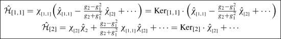
since it is sufficient for the operator \(\hat{h}_{[r]}\) to annihilate all Schur polynomials, except for \(\chi _{_{[r]}}\), thus it can be (and is) independent of the g-variables. However, the next operator \(\hat{\mathcal{H}}_{[r-1,1]}\) should annihilate not just \(\chi _{_{[r]}}\) but a g-dependent combination of \(\chi _{_{[r]}}\) and \(\chi _{_{[r-1,1]}}\), which enters \(\mathrm{Ker}_{[r]}\), and thus it needs to depend on g. However, the only Kerov function, which contains \(\chi _{_{[r-1,1]}}\), and differs from \(\mathrm{Ker}_{[r-1,1]}\) is \(\mathrm{Ker}_{[r]} = \chi _{_{[r]}} + \mathcal{K}_{[r],[r-1]}^{(g)}\chi _{_{[r-1,1]}} + \cdots \), thus
An explicit example of this phenomenon is the coincidence of two underlined operators in (79), as well as the coefficient in front of the last term in the second expression for \(\hat{\mathcal{H}}_{[2,1]}\). In general, \(\mathcal{H}_Q\) are related to \(\hat{h}_Q\) by an upper triangular transformation with the transposed inverse of the Kostka–Kerov matrix:
Indeed, then
One can substitute expansion (32) into (39), which provides
There is no sum over Q. Performing the sum, one gets the identity operator
which leaves every Schur polynomial, and hence every Macdonald and Kerov ones, intact:
For the dual Kerov functions, one gets their own Hamiltonians
and there are obvious operators which convert \(\mathrm{Ker}\) into \(\widetilde{\mathrm{Ker}}\) and back:
9. Our next task is to construct the g-independent operators \(\hat{h}_S\) explicitly. Note that \(\hat{h}_{_S} = \hat{\chi }_{_S} + \cdots \) with non-trivial corrections, because we do not put all \(p_k=0\) in (36), thus the standard orthogonality condition, mentioned in the first paragraph of Sect. 4 is not enough.
Already the very first operator \(\hat{h}_{[1]}\) has quite an inspiring form clearly seen in the first line of (79):
Generalization is obvious, and it is indeed true: for arbitrary Q
To prove (36), one can apply the Cauchy formula (15) in the form
to
Then at the l.h.s., we get a shift of \(p'\) by \(-p\), and putting \(p'=0\) afterwards reduces it to \(\chi _{_R}\{p''\}\). Comparison with the r.h.s. gives:
The last bracket imposes the condition that \(Y\in Q\otimes X^\vee \), and, comparing the terms with \(\chi _{_Q}\{p''\}\) at both sides, we obtain the desired relation
Note that the contributing to the sum at \(Q=R\) is just the term with \(X=\emptyset \).
Equations (39) and (47) give a complete explicit construction of Hamiltonians for the Kerov functions (and in fact for any system of symmetric functions defined by a linear transformation of Schur polynomials with the matrix \(\mathcal{K}\)).
This is, however, not yet the case when the dream came true. The naive Hamiltonians (39) depend explicitly on the Kostka–Kerov matrix, and can not be used to derive it. At the same time, in the Macdonald case, there were very special Ruijsenaars Hamiltonians (6), which do not refer to the Kostka matrix, and could be used for its derivation. Despite this is technically much harder than using the orthogonalization procedure, still it is conceptually important that such Hamiltonians exist. We do not discuss here what is so special about (6) and what are the chances to find their counterparts in the Kerov case.
10. The Ruijsenaars Hamiltonian (6) was described by a maximally degenerate (factorized) matrix \(\xi _{_{X,Y}}\), but instead it had no free parameters in the set of eigenvalues, i.e. even in Macdonald case it was some peculiar combination of our Hamiltonians \(\hat{\mathcal{H}}_Q\). In fact, to get the exponential Hamiltonian (6), one should just substitute the eigenvalues (7) into (35) and (41) and restrict the Kostka–Kerov matrix \(\mathcal{K}\) to the Macdonald locus. However, since eigenvalues depend on Q, one needs a generalization of the sum rule (42). Our next goal is to reveal in the simplest example of the Appendix what is a peculiar combination of \(\hat{\mathcal{H}}_Q\) leading to (6), and to explain why the same factorizability (rank one) condition can not be imposed outside the Macdonald locus (3). We can also look at the weakened, say, rank-two condition and find what is the corresponding extension of the Macdonald locus. In fact, matrix \(\xi _{_{X,Y}}\) is not of rank 1 already at level 2, see (74). However, one can make it degenerate by adjusting one of the three eigenvalues:
One can repeat this trick at level 3, then all the three eigenvalues get expressed through \(E_{[1]}\) and \(E_{[2]}\):
Moreover, at this locus (in E-space) we get quite a nice factorized formula
which reproduces (6) at the Macdonald locus (3) in the g-space, but does not work beyond it, starting from level 4, where a two-hook diagram emerges for the first time. Let us emphasize again that (54) should be considered not freely, but for the eigenvalues restricted by conditions (52), (53), etc, which, on the Macdonald locus, reduce to (7). We do not know how to deform such a simple formula as Eq. (54) beyond the Macdonald locus, at least the Kerov functions are not the eigenfunctions of the operators that one can build from this \(\xi ^\mathrm{fact}\). Note also that even if (54) would be true, it satisfies (25) with the sum upper limit \(M=1\) but not obligatory (26), i.e. the necessary conditions for an exponential Hamiltonian to exist would not be fulfilled.
11. The question, however, remains, if one can get an exponential Hamiltonian with \(M>1\). One option here is to look for generalizations of the Macdonald locus (3) with the hope that some factorization properties survive. Indeed, since the vanishing property (20) played a role in construction of exponential Hamiltonians, it is instructive that it has a generalization to other loci:
which is a simple corollary of the general theorem: the Schur polynomial \(\chi _{_R}\) is non-zero at \(p_k=\sum _{i=1}^Nx_i^k-\sum _{i=1}^Ny_i^k\) iff R has no more than N hooks. One of the simplest ways to prove this theorem is to realize such a Schur polynomial as a fermionic average of a product of fermions: \(\chi _{_R}=\Big <\prod _{i=1}^N\psi ^*(y_i)\psi (x_i)\cdot \prod _{a}^N\psi _{-\mu _a}^*\psi _{\nu _a}\Big>\), where \(\mu _a\) are lengths of the vertical hook legs, and \(\nu _a+1\) are lengths of the horizontal ones [66]. One can also prove the theorem using the hook determinant formula from the Appendix.
The properties (55) support the hope for factorization. As already mentioned in Sect. 6, the first series \(p_k =\frac{\{t^{mk}\}}{\{t^k\}}\cdot \{q^k\}\) appears in study of the higher Ruijsenaars Hamiltonians. The second series \(p_k = \prod _{a=1}^m\{q_a^k\}\) is naturally relevant for considerations at the Freund–Zabrodin [41] locus
in the space of Kerov times \(g_k\). We leave a detailed analysis of this possibility for the future.
12. Another question which we mentioned in the beginning of this text is if one can define generalized functions with the help of \(\hat{\mathcal{H}}_Q\)? Of course, for any system of, say, two-point generalized functions
defined by a triangular transformation of the bi-linear Schur basis, there is a direct generalization of (35) and (39):
which defines a Hamiltonian for arbitrary set of the eigenvalues:
The question is, however, to find a restricted sub-set of Hamiltonians which could be described with no explicit reference to the generalized Kostka–Kerov matrix \(\mathcal{K}\) and thus could be used to define it.
In the Macdonald case, such interesting Hamiltonians exist [53, 54], and are given by simple sums of Ruijsenaars exponential Hamiltonians with a simple triangular mixing of time sets \(\{p\}\) and \(\{p'\}\). More precisely, the first one is obtained from (6) and (19) by the transformation
with the deformation parameter \(A^{-2}\). At the Macdonald locus, the mixing is \(p'_k+\epsilon _kp_k\) with \(\epsilon _k = 1 - \Big (\frac{t}{q}\Big )^{2k} \) made from the third item of the DIM triple \(q,t^{-1},tq^{-1}\) [34].
13. To conclude, in this paper we constructed a full set of Hamiltonians for Kerov functions. This is a superficially large set, and it can not help to define the functions per se, because our Hamiltonians explicitly contain the Kostka–Kerov matrix, i.e. they use it as an input rather than serve as a tool to define the Kerov functions. In other terms, they demonstrate super-integrability, but lack the advantage of (6) and its relatives, which formed a smaller set of operators depending on parameters q and t in a simple explicit way, not through the Kostka–Macdonald matrix, and thus could serve its definition. The fact that the peculiar properties of the Hamiltonians in the Schur case have generalizations to other loci gives a hope to lift the construction, say, to the Freund–Zabrodin generalizations of the Macdonald locus, but this is beyond the scope of the present paper. Our main goal was to demonstrate that the notion of Kerov Hamiltonians has a clear meaning, and to make a setting for the next attacks on this interesting problem.
Data Availability Statement
This manuscript has no associated data or the data will not be deposited. [Authors’ Comment: This is a theoretical study and no experimental data has been listed.]
Notes
Throughout this paper, we use the standard group/knot theory notation: for the Young diagram \(\Delta = \left[ \delta _1\ge \delta _2\ge \cdots \ge \delta _{l_\Delta }>0\right] = \big [\ldots ,\underbrace{2,\ldots ,2}_{m_2}, \underbrace{1,\ldots , 1}_{m_1}\big ]\), the size (level) is \(|\Delta | = \sum _{i=1}^{l_\Delta } \delta _i = \sum _a am_a\), the time-monomial is \(p_\Delta := \prod _{i=1}^{l_\Delta } p_{\delta _i}\), and combinatorial factor is \(z_\Delta = \prod _{a} a^{m_a} m_a! \). Also, \(\{x\} :=x-x^{-1}\). We deal with the Schur, Macdonald polynomials and the Kerov functions, which are symmetric polynomials of variables \(x_i\) as functions of time variables \(p_k:=\sum _ix_i^k\), they are labeled by Young diagrams, we use the notation \(\chi _R\{p\} = \mathrm{Schur}_R\{p\}\) for the Schur polynomials.
It can be obtained using (63) from

In the simplest way, this latter is obtained from the generating function of symmetric Young diagrams in this case:

i.e.
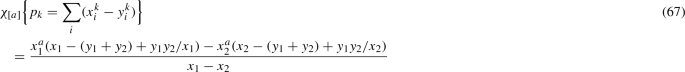
with \(x_1=qt\), \(x_2=q/t\), \(y_1=t/q\), \(y_2=1/(qt)\).


References
L. Alday, D. Gaiotto, Y. Tachikawa, Lett. Math. Phys. 91, 167–197 (2010). arXiv:0906.3219
N. Wyllard, JHEP 0911, 002 (2009). arXiv:0907.2189
A. Mironov, A. Morozov, Nucl. Phys. B 825, 1–37 (2009). arXiv:0908.2569
H. Awata, B. Feigin, A. Hoshino, M. Kanai, J. Shiraishi, S. Yanagida, arXiv:1106.4088
Y. Ohkubo, H. Awata, H. Fujino, arXiv:1512.08016
M. Fukuda, Y. Ohkubo, J. Shiraishi, arXiv:1903.05905
A. Mironov, A. Morozov, Sh Shakirov, JHEP 1102, 067 (2011). arXiv:1012.3137
V. Alba, V. Fateev, A. Litvinov, G. Tarnopolsky, Lett. Math. Phys. 98, 33–64 (2011). arXiv:1012.1312
A. Mironov, A. Morozov, S. Shakirov, A. Smirnov, Nucl. Phys. B 855, 128 (2012). arXiv:1105.0948
A. Morozov, A. Smirnov, Lett. Math. Phys. 104, 585 (2014). arXiv:1307.2576
S. Mironov, An Morozov, Y. Zenkevich, JETP Lett 99, 109 (2014). arXiv:1312.5732
Y. Ohkubo, arXiv:1404.5401
Y. Kononov, A. Morozov, Eur. Phys. J. C 76, 424 (2016). arXiv:1607.00615
Y. Zenkevich, arXiv:1612.09570
M. Aganagic, Sh. Shakirov, arXiv:1105.5117; arXiv:1210.2733
P. Dunin-Barkowski, A. Mironov, A. Morozov, A. Sleptsov, A. Smirnov, JHEP 03, 021 (2013). arXiv:1106.4305
I. Cherednik, arXiv:1111.6195
A. Mironov, A. Morozov, An Morozov, JHEP 1203, 034 (2012). arXiv:1112.2654
A. Mironov, A. Morozov, Sh Shakirov, A. Sleptsov, JHEP 2012, 70 (2012). arXiv:1201.3339
A. Mironov, A. Morozov, Sh Shakirov, J. Phys. A: Math. Theor. 45, 355202 (2012). arXiv:1203.0667
A. Mironov, A. Morozov, An. Morozov, in: Strings, Gauge Fields, and the Geometry Behind: The Legacy of Maximilian Kreuzer, eds: A. Rebhan, L. Katzarkov, J. Knapp, R. Rashkov, E. Scheidegger, World Scietific, 2013 pp.101-118 arXiv:1112.5754 (2013)
S.-S. Chern, J. Simons, Ann. Math. 99, 48–69 (1974)
E. Witten, Commun. Math. Phys. 121, 351–399 (1989)
J.W. Alexander, Trans. Am. Math. Soc. 30(2), 275–306 (1928)
V.F.R. Jones, Invent. Math. 72, 1 (1983)
V.F.R. Jones, Bull. AMS 12, 103 (1985)
V.F.R. Jones, Ann. Math. 126, 335 (1987)
L. Kauffman, Topology 26, 395 (1987)
P. Freyd, D. Yetter, J. Hoste, W.B.R. Lickorish, K. Millet, A. Ocneanu, Bull. AMS. 12, 239 (1985)
J.H. Przytycki, K.P. Traczyk, Kobe J. Math. 4, 115–139 (1987)
J.H. Conway, Algebraic Properties, In: John Leech (ed.), Computational Problems in Abstract Algebra, Proc. Conf. Oxford, 1967, Pergamon Press, Oxford-New York, 329-358, (1970)
I.G. Macdonald, Symmetric functions and Hall polynomials, 2nd edn. (Oxford University Press, Oxford, 1995)
H. Awata, B. Feigin, J. Shiraishi, JHEP 1203, 041 (2012). arXiv:1112.6074
H. Awata, H. Kanno, T. Matsumoto, A. Mironov, A. Morozov, A. Morozov, Y. Ohkubo, Y. Zenkevich, JHEP 1607, 103 (2016). arXiv:1604.08366
H. Awata, H. Kanno, A. Mironov, A. Morozov, A. Morozov, Y. Ohkubo, Y. Zenkevich, JHEP 1610, 047 (2016). arXiv:1608.05351
J. Ding, K. Iohara, Lett. Math. Phys. 41, 181–193 (1997). arXiv:q-alg/9608002
K. Miki, J. Math. Phys. 48, 123520 (2007)
Y. Zenkevich, arXiv:1712.10300
A. Morozov, Phys. Lett. B785, 175-183 (2018) arXiv:1808.01059; arXiv:1810.00395
S.V. Kerov, Func. An. and Apps. 25, 78–81 (1991)
P.G.O. Freund, A.V. Zabrodin, Phys. Lett. B 294, 347–353 (1992). arXiv:hep-th/9208063
T.H. Baker, Symmetric functions and infinite-dimensional algebras, PhD Thesis, 1994, Tasmania (1994)
A.H. Bougourzi, L. Vinet, Lett. Math. Phys. 39, 299–311 (1997). arXiv:q-alg/9604021
A.A. Bytsenko, M. Chaichian, R.J. Szabo, A. Tureanu, arXiv:1308.2177
A.A. Bytsenko, M. Chaichian, R. Luna, J. Math. Phys. 58, 121701 (2017). arXiv:1707.01553
A. Mironov, A. Morozov, arXiv:1811.01184
S.N.M. Ruijsenaars, H. Schneider, Ann. Phys. (NY) 170, 370 (1986)
S.N.M. Ruijsenaars, Comm. Math. Phys. 110, 191–213 (1987)
S.N.M. Ruijsenaars, Commun. Math. Phys. 115, 127–165 (1988)
H. Awata, Y. Matsuo, S. Odake, J. Shiraishi, Phys. Lett. B 347, 49–55 (1995). arXiv:hep-th/9411053
M. Haiman, in: New Perspectives in Geometric Combinatorics, MSRI Publications 37, 207-254 (1999)
J. Shiraishi, Comm. Math. Phys. 263, 439–460 (2006)
A. Mironov, A. Morozov, arXiv:1907.05410
A. Mironov, A. Morozov, Y. Zenkevich, to appear
A. Mironov, A. Morozov, S. Natanzon, Theor. Math. Phys. 166, 1–22 (2011). arXiv:0904.4227
A. Mironov, A. Morozov, S. Natanzon, J. Geometry Phys. 62, 148–155 (2012). arXiv:1012.0433
D. Goulden, D.M. Jackson, A. Vainshtein, Ann. Comb. 4, 27–46 (2000). Brikhäuser, arXiv:math/9902125
V. Ivanov, S. Kerov, J. Math. Sci. (Kluwer) 107, 4212–4230 (2001). arXiv:math/0302203
A. Mironov, A. Morozov, S. Natanzon, arXiv:1904.11458
A. Morozov, Theor. Math. Phys. 200, 938–965 (2019). arXiv:1810.00395
A. Mironov, A. Morozov, JHEP 08, 163 (2018). arXiv:1807.02409
A. Morozov, arXiv:1906.09971
A. Mironov, A. Morozov, arXiv:1912.00635
A. Morozov, Eur. Phys. J. C 79(1), 76 (2019). arXiv:1812.03853
A. Mironov, A. Morozov, Nucl. Phys. B 944, 114641 (2019). arXiv:1903.00773
M. Kashiwara, T. Miwa, Proc. Japan cad. A 57, 342–347 (1981)
E. Date, M. Jimbo, M. Kashiwara, T. Miwa, J. Phys. Soc. Jpn. 50, 3806–3812 (1981)
http://knotebook.org.s3-website-us-west-2.amazonaws.com/knotebook/KerMacData/kermac.htm
Acknowledgements
This work was supported by the Russian Science Foundation (Grant No.16-12-10344).
Author information
Authors and Affiliations
Corresponding author
Appendix
Appendix
Schur polynomials as determinants of the hook constituents. Here we write down the determinant representation of the Schur polynomials in terms of hook constituents following [66, 67]. These formulas are convenient for dealing with diagrams with a restricted number of hooks.
First of all, let us note that, as follows from the Cauchy formula (15),
On the other hand, since \(N_{[a],[1^]}^X=\delta _{X,[a,1^b]}+\delta _{X,[a+1,1^{b-1}]}\) and \(\chi _{_X}\{p_k\}= (-1)^{|X|}\chi _{_{X^\vee }}\{-p_k\}\),
Then, for the Young diagram R consisting of n hooks with vertical leg length \(b_i+1\), and horizontal leg lengths \(a_i\), \(i=1\ldots n\), the Schur polynomial reads
An example: the second Macdonald Hamiltonian. Here we demonstrate in detail how the formulas work in the case of the second Macdonald Hamiltonian (29).
In the first term of (29), non-vanishing are contributions of 1-hook diagrams withFootnote 2
and of the two-hook diagrams with (using (64))
As for the second term, the product of two \(V_1\) is
When this operator acts on particular \(\chi _{_R}\) only a few terms in the last two brackets contribute, providing a polynomial in \(z_{1}^{-1}\) and \(z_2^{-1}\) of the common degree |R|. For example, the action on \(\chi _{[1,1]}=\mathrm{Mac}_{_{[1,1]}}\) gives
Now we need to multiply by the first two brackets, but pick up only the terms of total grading zero, since they will be selected by the contour integrals over \(z_1\) and \(z_2\):
It remains to substitute the integrals
to get
This answer contains both \(\chi _{_{[2]}}\) and \(\chi _{_{[1,1]}}\), thus \(\chi _{_{[1,1]}}=\mathrm{Mac}_{_{1,1]}}\) is not an eigenfunction of integrated \(:{\hat{V}}_1(z_1){\hat{V}}_1(z_2):\) This is cured by adding \(\oint \frac{dz}{z} \,{\hat{V}}_2(z)\):
Together they provide an answer, proportional to \(\chi _{_{[1,1]}}=\mathrm{Mac}_{_{1,1]}}\):
An example: Hamiltonians \(\mathcal{H}_Q\) at the first three levels. Here we consider the first three levels in order to illustrate the construction of the Hamiltonians \(\mathcal{H}_Q\). Note that (33) are formulated entirely in terms of skew Schur polynomials, what makes the calculations easy (once the Kostka–Kerov matrix is available from [68]).
Level 1. Here \(R=1\), \(\mathrm{Ker}_{[1]}=p_1\) and \(\boxed {\xi _{[1],[1]}=E_{[1]}}\)
Level 2. This example is already informative. We have two Kerov functions \(\mathrm{Ker}_{[1,1]}=\frac{p_2+p_1^2}{2}=\chi _{[1,1]}\) and \(\mathrm{Ker}_{[2]} =\chi _{[2]}+\frac{g_2-g_1^2}{g_2+g_1^2}\cdot \chi _{[1,1]} = \frac{-g_1^2p_2+g_2p_1^2}{g_2+g_1^2}\). Thus the two equations in (33) are:
$$\begin{aligned}&(\hat{\mathcal{H}}-E_{[1,1]})\mathrm{Ker}_{[1,1]} = \xi _{_{[1],[1]}}\chi _{_{[1]}}^2 + \xi _{_{[2],[1,1]}}\chi _{_{[2]}}\nonumber \\&\quad +(\xi _{_{[1,1]}}-E_{[1,1]})\chi _{_{[1,1],[1,1]}} = 0 \nonumber \\&(\hat{\mathcal{H}}-E_{[2]})\mathrm{Ker}_{[2]} = \left( \xi _{_{[1],[1]}}\chi _{_{[1]}}^2 + (\xi _{_{[2],[2]}}-E_{[2]})\chi _{_{[2]}}\right. \nonumber \\&\quad \left. +\xi _{_{[1,1],[2]}}\chi _{_{[1,1]}}\right) \nonumber \\&\quad +\frac{g_2-g_1^2}{g_2+g_1^2}\left( \xi _{_{[1],[1]}}\chi _{_{[1]}}^2 + \xi _{_{[2],[1,1]}}\chi _{_{[2]}}\right. \nonumber \\&\quad \left. +(\xi _{_{[1,1],[1,1]}}-E_{[2]})\chi _{_{[1,1]}}\right) = 0 \end{aligned}$$(72)We used here the fact that \(\chi _{_{[2]/[1]}}=\chi _{_{[1,1]/[1]}}\) and can further use \(\chi _{_{[1]}}^2=\chi _{_{[2]}}+\chi _{_{[1,1]}}\). Moreover, the first equation implies that, in the last line, we can substitute the bracket for just \((E_{[1,1]}-E_{[2]})\chi _{_{[1,1]}}\), i.e. a non-trivial g-dependence appears only in the coefficient of \(\chi _{_{[1,1],[1,1]}}\), not of \(\chi _{_{[2]}}\). In other words, we get a system
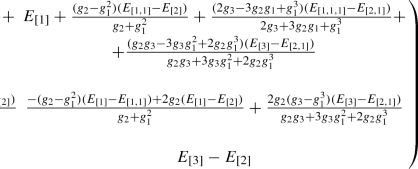
$$\begin{aligned} \xi _{_{[1,1],[1,1]}}= & {} E_{[1,1]}-\xi _{_{[1],[1]}} = E_{[1,1]}-E_{[1]}\nonumber \\ \xi _{_{[2],[1,1]}}= & {} -\xi _{{[1],[1]}}=-E_{[1]}\nonumber \\ \xi _{_{[1,1],[2]}}= & {} \frac{g_2-g_1^2}{g_2+g_1^2}(E_{[2]}-E_{[1,1]}) - E_{[1]}\nonumber \\ \xi _{_{[2],[2]}}= & {} E_{[2]}-\xi _{_{[1],[1]}} = E_{[2]}-E_{[1]} \end{aligned}$$(73)and
$$\begin{aligned} \xi = \left( \begin{array}{ccc} &{}\\ E_{[1,1]}-E_{[1]} &{}&{} -E_{[1]} \\ &{}\\ \frac{g_2-g_1^2}{g_2+g_1^2}(E_{[2]}-E_{[1,1]}) - E_{[1]} &{}\ \ &{} E_{[2]}-E_{[1]} \\ &{}\\ \end{array} \right) \end{aligned}$$(74)Thus, at this level, we can already collect all the terms proportional to \(E_{[1]}\), and reveal the structure of the simplest Hamiltonian (34):
 (75)
(75)associated with the eigenvalue \(E_{[1]}\): it annihilates all \(\chi _{_R}\) except for \(\chi _{_{[1]}}\),
$$\begin{aligned} \hat{\mathcal{H}}_{[1]}\chi _{_R} = \chi _{_R}\cdot \delta _{R,[1]} \end{aligned}$$(76)Also seen at level two are the two other Hamiltonians, but only the first terms can be defined:
 (77)
(77)Note that, while \(\hat{\mathcal{H}}_{[2]}\) annihilates \(\chi _{[1,1]}=\mathrm{Ker}_{[1,1]}\), the other Hamiltonian \(\hat{\mathcal{H}}_{[1,1]}\) annihilates not \(\chi _{[2]}\), but \(\mathrm{Ker}_{[2]} \sim \chi _{_{[2]}} + \frac{g_2-g_1^2}{g_2+g_1^2}\,\chi _{_{[1,1]}}\).
Level 3. Now
$$\begin{aligned} \mathrm{Ker}_{[1,1,1]}= & {} \chi _{_{[1,1,1]}} \nonumber \\ \mathrm{Ker}_{[2,1]}= & {} \chi _{_{[2,1]}} + \frac{2(g_3-g_1^3)}{2g_3+3g_2g_1+g_1^3}\,\chi _{_{[1,1,1]}}\nonumber \\ \mathrm{Ker}_{[3]}= & {} \chi _{_{[3]}} + \frac{2g_2(g_3-g_1^3)}{g_3g_2+3g_3g_1^2+2g_2g_1^3}\, \chi _{_{[2,1]}}\nonumber \\&+ \frac{g_3g_2-3g_3g_1^2+2g_2g_1^3}{g_3g_2+3g_3g_1^2+2g_2g_1^3}\, \chi _{_{[1,1,1]}} \end{aligned}$$(78)From these formulas, one can calculate the level-3 block of the matrix \(\xi _{_{X,Y}}\):
Now one can read off the level-three contributions to the Hamiltonians:
$$\begin{aligned} \hat{\mathcal{H}}_{[1]}= & {} \chi _{_{[1]}}\hat{\chi }_{_{[1]}} - (\chi _{_{[1,1]}}+\chi _{_{[2]}}) (\hat{\chi }_{_{[1,1]}}+\hat{\chi }_{_{[2]}}) \nonumber \\&+(\chi _{_{[2,1]}}+\chi _{_{[3]}})\hat{\chi }_{_{[1,1,1]}} \nonumber \\&+ (\chi _{_{[1,1,1]}}+2\chi _{_{[2,1]}} +\chi _{_{[3]}})\hat{\chi }_{_{[2,1]}}\nonumber \\&+ (\chi _{_{[1,1,1]}}+\chi _{_{[2,1]}})\hat{\chi }_{_{[3]}} + \cdots \nonumber \\= & {} \mathrm{Ker}_{[1]}\cdot \Big (\hat{\chi }_{_{[1]}} - \chi _{_{[1]}} \cdot (\hat{\chi }_{_{[2]}}+\hat{\chi }_{_{[1,1]}}) \nonumber \\&+ \chi _{_{[1,1 ]}}(\hat{\chi }_{_{[2,1]}}+ \hat{\chi }_{_{[3]}}) \nonumber \\&+ \chi _{_{[2 ]}}( \hat{\chi }_{_{[1,1,1]}} + \hat{\chi }_{_{[2,1]}}) + \cdots \Big ) \nonumber \\ \hat{\mathcal{H}}_{[1,1]}= & {} \chi _{_{[1,1]}} \Big (\hat{\chi }_{_{[1,1]}} - \frac{g_2-g_1^2}{g_2+g_1^2}\,\hat{\chi }_{_{[2]}} \Big ) \nonumber \\&- (\chi _{_{[1,1,1]}}+\chi _{_{[2,1]}}) \nonumber \\&\left( (\hat{\chi }_{_{[1,1,1]}}+\hat{\chi }_{_{ [2,1]}}) \right. \nonumber \\&\left. + \frac{g_2-g_1^2}{g_2+g_1^2}\,(\hat{\chi }_{_{[2,1]}}+\hat{\chi }_{_{[3]}}) \right) + \cdots \nonumber \\= & {} \mathrm{Ker}_{[1,1]}\nonumber \\&\cdot \left( \Big (\hat{\chi }_{_{[1,1]}} - \chi _{_{[1]}}(\hat{\chi }_{_{ [1,1,1]}}+\hat{\chi }_{_{ [2,1]}}) +\cdots \Big ) \right. \nonumber \\&\left. - \frac{g_2-g_1^2}{g_2+g_1^2}\cdot \Big (\underline{\hat{\chi }_{_{[2]}} - \chi _{_{[1]}}(\hat{\chi }_{_{ [2,1]}}+\hat{\chi }_{_{[3]}})+\cdots }\Big )\right) \nonumber \\ \hat{\mathcal{H}}_{[2]}= & {} \left( \chi _{_{[2]}} + \frac{g_2-g_1^2}{g_2+g_1^2}\,\chi _{_{[1,1]}}\right) \hat{\chi }_{_{[2]}}\nonumber \\&- \left( ( \chi _{_{[2,1]}}+ \chi _{_{[3]}})+ \frac{g_2-g_1^2}{g_2+g_1^2}\,(\chi _{_{[1,1,1]}}+\chi _{_{[2,1]}})\right) \nonumber \\&(\hat{\chi }_{_{[1,2]}}+\hat{\chi }_{_{[3]}}) +\cdots \nonumber \\= & {} \mathrm{Ker}_{[2]}\cdot \Big (\underline{\hat{\chi }_{_{[2]}} - \chi _{_{[1]}}\cdot (\hat{\chi }_{_{[1,2]}}+\hat{\chi }_{_{[3]}}) + \cdots }\Big )\nonumber \\ \hat{\mathcal{H}}_{[1,1,1]}= & {} \chi _{_{[1,1,1]}}\cdot \left( \hat{\chi }_{_{[1,1,1]}} -\frac{ 2(g_3-g_1^3) }{2g_3+3g_2g_1+g_1^3}\,\hat{\chi }_{_{[2,1]}}\right. \nonumber \\&\left. + \frac{2g_3-3g_2g_1+g_1^3}{2g_3+3g_2g_1+g_1^3} \, \hat{\chi }_{_{[3]}}\right) \nonumber \\&+\cdots \hat{\mathcal{H}}_{[2,1]} = \chi _{_{[2,1]}}\hat{\chi }_{_{[2,1]}} \nonumber \\&+ \frac{2(g_3-g_1^3) }{2g_3+3g_2g_1+g_1^3}\,\chi _{_{[1,1,1]}}\hat{\chi }_{_{[2,1]}} \nonumber \\&-\frac{2g_2(g_3-g_1^3) }{g_2g_3+3g_3g_1^2+2g_2g_1^3}\,\chi _{_{[2,1]}} \cdot \hat{\chi }_{_{[3]}} \nonumber \\&- \left( \frac{2g_3-3g_2g_1+g_1^3 }{2g_3+3g_2g_1+g_1^3}\right. \nonumber \\&\left. +\frac{g_2g_3-3g_3g_1^2+2g_2g_1^3 }{g_2g_3+3g_3g_1^2+2g_2g_1^3}\right) \chi _{_{[1,1,1]}}\cdot \hat{\chi }_{_{[3]}} +\cdots \nonumber \\= & {} \mathrm{Ker}_{[2,1]} \nonumber \\&\cdot \left( \hat{\chi }_{_{[2,1]}} - \frac{2g_2(g_3-g_1^3) }{g_2g_3+3g_3g_1^2+2g_2g_1^3}\,\hat{\chi }_{_{[3]}} + \cdots \right) \nonumber \\ \hat{\mathcal{H}}_{[3]}= & {} \left( \frac{g_2g_3-3g_3g_1^2+2g_2g_1^3 }{g_2g_3+3g_3g_1^2+2g_2g_1^3}\, \chi _{_{[1,1,1]}} \right. \nonumber \\&\left. +\frac{2g_2(g_3-g_1^3) }{g_2g_3+3g_3g_1^2+2g_2g_1^3} \, \chi _{_{[2,1]}} + \chi _{_{[3]}}\right) \nonumber \\&\cdot \hat{\chi }_{_{[3]}} +\cdots = \mathrm{Ker}_{[3]}\cdot \hat{\chi }_{_{[3]}} +\cdots \end{aligned}$$(79)


Rights and permissions
Open Access This article is licensed under a Creative Commons Attribution 4.0 International License, which permits use, sharing, adaptation, distribution and reproduction in any medium or format, as long as you give appropriate credit to the original author(s) and the source, provide a link to the Creative Commons licence, and indicate if changes were made. The images or other third party material in this article are included in the article’s Creative Commons licence, unless indicated otherwise in a credit line to the material. If material is not included in the article’s Creative Commons licence and your intended use is not permitted by statutory regulation or exceeds the permitted use, you will need to obtain permission directly from the copyright holder. To view a copy of this licence, visit http://creativecommons.org/licenses/by/4.0/.
Funded by SCOAP3
About this article

Cite this article
Mironov, A., Morozov, A. On Hamiltonians for Kerov functions. Eur. Phys. J. C 80, 277 (2020). https://doi.org/10.1140/epjc/s10052-020-7811-3
Received:
Accepted:
Published:
DOI: https://doi.org/10.1140/epjc/s10052-020-7811-3