 collaboration
Abstract
We present the open-source package openQ*D-1.0 (openQ*D. GitLab: https://gitlab.com/rcstar/openQxD. CSIC: https://dx.doi.org/10.20350/digitalCSIC/8591. https://hdl.handle.net/10261/173334, 2019), which has been primarily, but not uniquely, designed to perform lattice simulations of QCD+QED and QCD, with and without \(\mathrm {C}^*\) boundary conditions, and O(a) improved Wilson fermions. The use of \(\mathrm {C}^*\) boundary conditions in the spatial direction allows for a local and gauge-invariant formulation of QCD+QED in finite volume, and provides a theoretically clean setup to calculate isospin-breaking and radiative corrections to hadronic observables from first principles. The openQ*D code is based on openQCD-1.6 (Simulation program for lattice QCD (openQCD code). https://cern.ch/luscher/openQCD, 2016) and NSPT-1.4 (Numerical Stochastic Perturbation Theory (NSPT code). https://cern.ch/luscher/NSPT, 2017). In particular it inherits from openQCD-1.6 several core features, e.g. the highly optimized Dirac operator, the locally deflated solver, the frequency splitting for the RHMC, or the 4th order OMF integrator.
1 Introduction
QED radiative corrections to hadronic observables are generally rather small but they become phenomenologically relevant when the target precision is at the percent level. For example, the leptonic and semileptonic decay rates of light pseudoscalar mesons are measured with a very high accuracy and, on the theoretical side, have been calculated with the required non-perturbative accuracy by many lattice collaborations. Most of these calculations have been performed by simulations of lattice QCD without taking into account QED radiative corrections. A recent review [4] of the results obtained by the different lattice groups shows that leptonic and semileptonic decay rates of \(\pi \) and K mesons are presently known at the sub-percent level of accuracy. At the same time, QED radiative corrections to these quantities are estimated to be of the order of a few percent, by means of chiral perturbation theory [5]. These estimates have recently been confirmed in the case of the leptonic decay rates of \(\pi \) and K by a first-principle lattice calculation of the QED radiative corrections at \(O(\alpha )\) in Refs. [6, 7].
Other remarkable examples of observables for which QED radiative corrections are phenomenologically relevant are the so-called lepton flavour universality ratios. For example \(R(D^{(*)})\) is defined as the branching ratio for \(B \mapsto D^{(*)} \ell {{\bar{\nu }}}_\ell \) with \(\ell =e,\mu \) divided by the branching ratio for \(B \mapsto D^{(*)} \tau {{\bar{\nu }}}_\tau \). Most of the hadronic uncertainties cancel in these ratios that are built in such a way that they are trivial in the Standard Model, in the limit in which the two leptons have the same mass. Presently, a combined analysis [8] of the R(D) and \(R(D^*)\) ratios shows a deviation of the experimental measurements from the theoretical predictions of the order of 3 standard deviations. On the other hand, QED radiative corrections are different for the two leptons because of the different masses and an improved theoretical treatment of these effects (see for example Refs. [9, 10] for a discussion of this point) can possibly enhance or reconcile the observed discrepancy between the experimental measurements and the theoretical expectations.
QED radiative corrections to hadronic observables can be computed from first principles by performing lattice simulations of QCD coupled to QED, treating the photon field on an equal footing as the gluon field. Since these corrections are expected to be at the percent level, in order to resolve them against the statistical noise, one needs to simulate at various values of the fine-structure constant and to interpolate to the physical value. This approach, pioneered in Refs. [11,12,13], is highly non-trivial from both the numerical and theoretical point of view, because of the peculiarities of QED. Numerically, lattice calculations are unavoidably affected by statistical and systematic uncertainties and it can be challenging to resolve QED radiative corrections from the leading QCD contributions within the errors of a simulation. Theoretically, a big issue arises because lattice calculations have necessarily to be done on a finite volume. QED is a long-range interaction and, consequently, finite-volume effects are the key issue in presence of electromagnetic interactions.
In fact, as a consequence of Gauss’ law, it is impossible to have a net electric charge on a periodic torus. Because of this strong theoretical constraint, it is particularly challenging to calculate from first principles physical observables associated with electrically charged external states, such as the phenomenologically relevant quantities discussed above. Several approaches have been proposed over the years to cope with this problem, see Ref. [14] for a recent review. The most popular approaches to the problem of charged particles on the torus solve the Gauss’ law constraint by introducing non-local terms in the finite-volume action of the theory.Footnote 1 The effects induced by the non-locality of the action are expected to disappear once the infinite-volume limit is properly taken and, as far as \(O(\alpha )\) QED radiative corrections are concerned, it is generally possible to show that this is indeed the case.
On the one hand, the non-local formulations of the theory are particularly appealing because of their formal simplicity. On the other hand, it has been shown in Ref. [18] that it is possible to probe electrically charged states on a finite volume by starting from a local formulation of the theory and, remarkably, in a fully gauge-invariant way. This is possible by using C-parity (or \(\mathrm {C}^*\)) boundary conditions for all the fields and by using a certain class of interpolating operators originally introduced by Dirac in a seminal work [19] on the canonical quantization of QED.
The formulation of Ref. [18] has also been studied numerically. The results for the meson masses extracted in a fully gauge-invariant way from lattice simulations of QCD+QED with \(\mathrm {C}^*\) boundary conditions obtained in Ref. [20] provide a convincing numerical evidence that, beside being an attractive theoretical formulation, the proposal of Ref. [18] is also a valid numerical alternative for the calculation of QED radiative corrections on the lattice. This motivated the present work.

Summary of salient features of openQ*D. Some features inherited from openQCD and NSPT are highlighted
In this paper we present the open-source package openQ*D, which can be used to simulate QCD+QED, QCD, the pure SU(3) and U(1) gauge theories.Footnote 2 The code allows to choose a wide variety of temporal and spatial boundary conditions. In particular, it allows to perform dynamical simulations of QCD+QED with \(\mathrm {C}^*\) but also with periodic boundary conditions along the spatial directions. Simulations of QCD with \(\mathrm {C}^*\) boundary conditions can be a valuable starting point for the application of the RM123 method [21], in which observables are calculated order-by-order in the electromagnetic coupling. A fully tested and stable release of openQ*D can be downloaded from [1].
The openQ*D package is based on the openQCD [2] package from which it inherits the core features, most notably the implementation of the Dirac operator, of the solvers and the possibility of simulating open and Schrödinger functional boundary conditions in the time direction. One of the inherited solvers implements the inexact deflation algorithm of Ref. [22]. An added value of the openQ*D package is the possibility of using more deflation subspaces in a single simulation. This is particularly important in the case of QCD+QED simulations because different deflation subspaces have to be generated for quarks having different electric charges.
Another important feature present in the openQ*D package is the possibility to use Fourier Acceleration [23, 24] for the molecular dynamics evolution of the U(1) field. The used implementation of the Fast Fourier Transform (FFT) is an adaptation of the corresponding module in the NSPT [3, 25] package.
The remaining of this paper is organised as follows. In Sect. 2 we give an overview of the theoretical background needed to understand the actions simulated by openQ*D, and we describe some peculiar aspects of the simulation algorithm. In particular, the specific implementation of \(\mathrm {C}^*\) boundary conditions and of the Fourier Acceleration for the U(1) field are discussed. In Sect. 3 we provide instructions on how to compile the code, construct a sample input file, and run the program that generates QCD+QED configurations. Section 4 is a collection of tests and performance studies. In particular, we present scalability tests, and studies of the performance of solvers for the Dirac equation for electrically charged fields. We also illustrate the outcome of some sample runs performed for testing purposes. In Fig. 1, we provide a schematic view of the openQ*D functionalities.
2 Theoretical background
An overview of the main algorithmic choices made in the code will be given in this section. The fundamental fields are the SU(3) link variable \(U_{\mu }(x)\) and the real photon field \(A_{\mu }(x)\). Since only the compact formulation of QED is implemented at present, all observables are written in terms of the U(1) link variable
which implies that the real photon field can be restricted to \(-\pi \le A_{\mu }(x) \le \pi \) with no loss of generality. Various boundary conditions can be chosen for the gauge fields: periodic, open [26], Schrödinger Functional (SF) [27, 28] and open-SF boundary conditions [29] in the Euclidean time direction \(\mu =0\), periodic and \(\mathrm {C}^*\) boundary conditions [30,31,32,33] in the spatial directions. The implementation of \(\mathrm {C}^*\) boundary conditions is discussed in Sect. 2.1.
After integrating out the fermion fields in a usual way, the target distribution of QCD+QED if no \(\mathrm {C}^*\) boundary conditions are used is
where the gauge actions \(S_{\mathrm {g,}\mathrm {SU}(3)}(U)\) and \(S_{\mathrm {g,}\mathrm {U}(1)}(A)\) are briefly discussed in Sect. 2.2, the product runs over the simulated fermion flavours indicized by f, and the Dirac operator D is introduced in Sect. 2.3. If \(\mathrm {C}^*\) boundary conditions are used, the determinant is replaced by a Pfaffian, i.e.
where C is the charge conjugation matrix and T is a field-independent matrix satisfying \(T^2=1\), whose detailed definition can be found in Sect. 2.1. While in the continuum limit the determinant and the Pfaffian are positive, this is not the case with Wilson fermions. The absolute value is considered in both cases, which amounts to replacing
The sign should be separately calculated and included in the evaluation of observables as a reweighting factor [34, 35]. It is important to stress that this is a mild sign problem [18], which becomes irrelevant sufficiently close to the continuum limit, and which is also present in standard QCD simulations for the strange quark. The presented strategy is in line with state-of-the-art QCD and QCD+QED simulations, in which the sign of the determinant is simply ignored. Future work will be planned to investigate the importance of the sign especially at lighter quark masses.
After introducing the standard even–odd preconditioned operator \(\hat{D}\) [36], one rewrites the quark part of the distribution as
where \(\alpha _f\) is either 1/2 or 1/4. The definitions of \(\hat{D}_f\) and \(S_{\mathrm {sdet}}\) can be found in Sect. 2.3. Instead of this target distribution, the openQ*D code simulates a slightly different distribution
written in terms of a rational approximation \(R_f\) [37]
where \({\mu }_f\) is a tunable parameter introduced to suppress configurations with exceptionally small eigenvalues of \(\hat{D}_f^\dag \hat{D}_f\) (twisted-mass reweighting [26, 38]). If \({\mu }_f\) is small enough and the rational approximation is accurate enough, the simulated distribution \(\rho _\mathrm {sim}(U,A)\) is very close to the target one \(\rho _\mathrm {tar}(U,A)\). The difference is corrected by means of reweighting factors \(W_f\)
which have to be separately calculated and included in the expectation values of observables as follows
The detailed discussion of the supported reweighting factors can be found in Appendix A. The rational function \(R_f\) can be decomposed in a product of positive factors \(R_{f,\ell }\) (frequency splitting [26]). More details on frequency splitting are provided in Sect. A.2. The determinant of the rational functions is finally represented by means of a pseudofermion quadratic action as in
The distribution is generated by means of a Hybrid Monte Carlo (HMC) algorithm with Fourier acceleration for the U(1) field. The molecular dynamics (MD) Hamiltonian is given by
where \(\Pi _\mu (x)\) and \(\pi _\mu (x)\) denote the momentum fields associated to the SU(3) and U(1) fields, the operator \((-\Delta )\) is a discretization of the Laplace operator, and the action is given by
Details on the implementation of the Fourier acceleration are presented in Appendix B. The HMC consists of three steps.
- 1.
The momentum and pseudofermion fields are randomly generated with probability distribution given by \(e^{-H}\);
- 2.
The gauge fields are evolved with a discretized version of the MD equations, i.e.
$$\begin{aligned} \partial _t A_\mu (x)&= \Delta ^{-1} \pi _\mu (x) \nonumber \\ \partial _t U_\mu (x)&= \Pi _\mu (x) U_\mu (x)\nonumber \\ \partial _t \pi _\mu (x)&= - \partial _{A_\mu (x)} S(U,A,\Phi ), \nonumber \\ \partial _t \Pi _\mu (x)&= - \partial _{U_\mu (x)} S(U,A,\Phi ), \end{aligned}$$(2.13)where \(\partial _{U_\mu (x)}\) is the left Lie derivative with respect to \(U_\mu (x)\) while \(\partial _{A_\mu (x)}\) is the elementary derivative with respect to \(A_\mu (x)\). In practice multiple time-scale [39] symplectic integrators are used to solve the MD equation: leapfrog, 2nd and 4th order Omelyan–Mryglod–Folk integrators [40] are available (LF, OMF2, OMF4).
- 3.
The evolved gauge configuration is accepted or rejected with a standard Metropolis test with probability distribution given by \(e^{-H}\).

Global geometry of extended lattice. The top diagram represents a section of the extended lattice along a (1, k) plane where \(k=2,3\) is a direction with \(\mathrm {C}^*\) boundary conditions. All fields are periodic along the extended direction 1. \(\mathrm {C}^*\) boundary conditions in the direction \(k=2,3\) are replaced by shifted boundary conditions in the extended lattice. Shifted boundary conditions are imposed by properly defining the nearest neighbours of boundary sites. Empty circles in the red (resp. green, blue) rectangle have to be identified with the corresponding solid circles in the red (resp. green, blue) rectangle. The bottom diagram represents a section of the extended lattice along a (1, k) plane where \(k=2,3\) is a periodic direction. In both diagrams, the black circles represent the sites of the physical lattice, and the grey circles represent the sites of the mirror lattice
2.1 \(\mathrm {C}^*\) boundary conditions
Other than the variety of boundary conditions in the temporal direction inherited from openQCD-1.6, the openQ*D code allows for periodic or \(\mathrm {C}^*\) boundary conditions to be chosen in the spatial directions. If the gauge fields satisfy periodic boundary conditions in all spatial directions k, the fermion fields \(\psi _f(x)\) and \({\bar{\psi }}_f(x)\) satisfy general phase-periodic boundary conditions (f is the flavour index), i.e.
Phase-periodic boundary conditions are incompatible with \(\mathrm {C}^*\) boundary conditions. If the gauge fields satisfy \(\mathrm {C}^*\) boundary conditions in at least one direction, say k, then \(\theta _{f,j}=0\) for all f and j, and
The charge-conjugation matrix C satisfies
\(\mathrm {C}^*\) boundary conditions are implemented by means of an orbifold construction. Assume that \(k=1\) is a direction with \(\mathrm {C}^*\) boundary conditions,Footnote 3 in order to simulate a physical lattice with size \(V = L_0 \times {L}_1 \times {L}_2 \times {L}_3\) the openQ*D code allocates a lattice with size \(V_{\mathrm {C}^*} = L_0 \times (2 {L}_1) \times {L}_2 \times {L}_3\), which we will refer to as the extended lattice. Points in the physical lattice are assumed to have coordinates which satisfy \(0 \le x_\mu < {L}_\mu \). The extended lattice can be interpreted as a double-covering of the physical lattice, with coordinates satisfying \(0 \le x_\mu < {L}_\mu \) for \(\mu \ne 1\) and \(0 \le x_1< 2{L}_1\). Points outside the physical lattice constitute the mirror lattice. On the extended lattice, points x and \(x + L_k {\hat{e}}_k\) do not coincide, so Eqs. (2.16) and (2.17) have to be interpreted as constraints which define the admissible gauge and fermion fields. These are referred to as the orbifold constraints. While the admissible gauge fields in the mirror lattice are completely determined by the value of the gauge field in the physical lattice via (2.16), the orbifold constraint has a different meaning for fermion fields, providing a relation between \(\psi \) in the physical lattice and \({\bar{\psi }}\) in the mirror lattice, and vice versa. Given that the fermion fields \(\psi \) and \({\bar{\psi }}\) are independent Grassmanian variables on the physical lattice, then one can equivalently choose the value of \(\psi \) in each point of the extended lattice as a complete set of independent variables. The integration of the Grassmanian variables yields the Pfaffian of the operator CTD [18], where T is the translation operator defined by
One easily proves that
which justifies the need for \(\alpha _f=1/4\) in Eq. (2.5). Since the square of the charge-conjugation operation is the identity, all fields must obey periodic boundary conditions along the extended direction \(k=1\), i.e.
\(\mathrm {C}^*\) boundary conditions in directions \(k = 2, 3\) are implemented by modifying the global topology of the extended lattice (see Fig. 2). In fact in these directions, \(\mathrm {C}^*\) boundary conditions in the physical lattice imply shifted boundary conditions in the extended lattice, i.e.
When the determinant of the Dirac operator is stochastically estimated by means of a pseudofermion action as in Eq. (2.12), the pseudofermion field \(\Phi _{f,\ell }\) is natively defined on the extended lattice, i.e. \(\Phi _{f,\ell }(x)\) are truly independent variables for each x in the extended lattice. Moreover it satisfies the same boundary conditions as \(\psi _f\) in Eqs. (2.22) and (2.24).
It is worth noticing that \(\mathrm {C}^*\) boundary conditions can be implemented in different ways. For instance, the implementation proposed in Appendix D of Ref. [18] does not double the lattice, but the number of pseudofermion fields. Roughly speaking one needs to represent quarks and antiquarks by means of independent pseudofermion fields which are mixed by the boundary conditions. The openQ*D implementation simply maps each pair of pseudofermion fields in the geometry of the extended lattice. The cost of the application of the Dirac operator implemented as in openQ*D and as in [18] is exactly identical. Therefore, as far as the application and inversion of the Dirac operator, the orbifold construction does not introduce any overhead with respect to more standard implementations of \(\mathrm {C}^*\) boundary conditions. On the other hand, the gauge field is evolved twice. In principle one could evolve the gauge field only on the physical lattice and then copy its value to the mirror lattice. This strategy will be considered in the future. However, simulations close to the physical point are dominated by the inversion of the Dirac operator and the overhead due to the evolution of the gauge field is expected to be negligible. Evidence of this fact has been presented in [41]. The orbifold construction has been chosen essentially because it requires only minimal modifications of the openQCD code. In fact the functions that impose the orbifold constraint on gauge and momentum fields are trivial, shifted boundary conditions (by half lattice) are implemented by a simple redefinition of the map of nearest neighbouring MPI processes, and finally gauge action and forces need to be multiplied by a factor 1/2. On the other hand the Dirac operators and the solvers are completely untouched by the orbifold construction.
2.2 Gauge actions
The SU(3) and compact U(1) gauge actions that can be simulated with openQ*D are
where \(U({\mathcal {C}})\) and \(z({\mathcal {C}})\) denote the SU(3) and U(1) parallel transports along a path \({\mathcal {C}}\) on the lattice. \({\mathcal {S}}_0\) and \({\mathcal {S}}_1\) are the sets of all oriented plaquettes and all oriented \(1 \times 2\) planar loops respectively and the overall weight \(\omega _{\mathrm {C}^*}\) is 1 if no \(\mathrm {C}^*\) boundary conditions are used. With \(\mathrm {C}^*\) boundary conditions \(\omega _{\mathrm {C}^*}=1/2\) corrects for the double counting introduced by summing over all plaquette and double-plaquette loops in the extended lattice instead of the physical lattice (c.f. Sect. 2.1). The coefficients \(c_{0,1}\) satisfy the relation \(c_0 + 8c_1 = 1\). For SU(3), the Wilson action is obtained by choosing \(c_0 = 1\), the tree-level improved Symanzik (or Lüscher–Weisz) action is obtained by choosing \(c_0 = \tfrac{5}{3}\), and the Iwasaki action is obtained by choosing \(c_0 = 3.648\). The parameters \(g_0\) and \(e_0\) are the bare SU(3) and U(1) gauge couplings respectively, which are related to the \(\beta \) parameter and the bare fine-structure constant \(\alpha _0\) by
In the compact formulation of QED, all electric charges must be integer multiples of some elementary charge \(q_\mathrm {el}\) which is defined in units of the charge of the positron. As discussed in Ref. [18], \(q_\mathrm {el}\) appears as an overall factor in the gauge action and essentially sets the normalization of the U(1) gauge field in the continuum limit. Even though in infinite volume \(q_\mathrm {el}=1/3\) would be an appropriate choice in order to simulate quarks, in finite volume with \(\mathrm {C}^*\) boundary conditions one needs to choose \(q_\mathrm {el}=1/6\) in order to construct gauge-invariant interpolating operators for charged hadrons [18, 20]. Note that by using a compact formulation of QED, no gauge fixing is added to the action, and furthermore the user is free to choose simulating (QCD+)QED without \(\mathrm {C}^*\) boundary conditions.
The actions in Eqs. (2.25) and (2.26) assume periodic boundary conditions in time. In the more general case, the actions are modified at the time boundary in order to allow for O(a) improvement. The general form of the gauge actions can be found in [42].
2.3 Dirac operator
The Dirac operator implemented in openQ*D is given by a sum of terms
where \(D_{\mathrm {w}}\) is the (unimproved) Wilson–Dirac operator, \(\delta D_{\mathrm {sw}}\) is the Sheikholeslami–Wohlert (SW) term, and \(\delta D_{\mathrm {b}}\) is the time boundary O(a)-improvement term. For simplicity, periodic boundary conditions in the time direction will be assumed, which means \(\delta D_{\mathrm {b}}=0\). The definition of \(\delta D_{\mathrm {b}}\) for other boundary conditions can be found in [43]. The Wilson–Dirac operator of Eq. (2.28) can be written as
where the covariant derivatives are defined as
The SW term is given by
The SU(3) field tensor \(\hat{F}_{\mu \nu }(x)\) and the U(1) field tensor \({\hat{A}}_{\mu \nu }(x)\) are constructed in terms of the clover plaquette. The explicit expression of the SU(3) field tensor used in openQ*D can be found in Ref. [44], while the U(1) field tensor is given here,
The normalization is chosen in such a way that \( -i e_0 \hat{A}_{\mu \nu }(x) \) is the canonically-normalized field tensor in the naive continuum limit. Notice that the field tensors are anti-hermitian.
In presence of electromagnetism, the Dirac operator depends on the electric charge of the quark field. Let q be the physical electric charge in units of e (i.e. \(q=2/3\) for the up quark, and \(q=-1/3\) for the down quark). In the compact formulation of QED, all electric charges must be integer multiples of an elementary charge \(q_\mathrm {el}\), which appears as a parameter in the U(1) gauge action (2.26). The integer parameter
is the one appearing in the hopping term in Eqs. (2.30) and (2.31). On the other hand, notice that the SW term (2.32) is written in terms of the physical charge q. This normalization corresponds to a definition of \(c_{\mathrm {sw}}^\mathrm {U(1)}\) which is equal to 1 at tree level. The definition of the even–odd preconditioned Dirac operator \(\hat{D}\) is standard [36]
and so is the definition of the small-determinant action \(S_{\mathrm {sdet}}\) appearing in Eq. (2.5)
3 Simulating QCD+QED with openQ*D
3.1 Structure of the openQ*D program package
The openQ*D code includes several main programs, roughly divided in three categories: programs to generate configurations, programs to measure observables, and utility programs. The following programs (in the main directory) can be used to generate gauge configurations for various theories:
iso1: SU(3)\(\times \)U(1) gauge theory with dynamical fermions;
qcd1: SU(3) gauge theory with dynamical fermions;
ym1: SU(3) pure gauge theory;
mxw1: U(1) pure gauge theory.
The following programs (in the main directory) can be used to calculate simple observables:
ms2: spectral range of \((\hat{D}^\dag \hat{D})^{1/2}\) (\(\hat{D}\) is the even–odd preconditioned Dirac operator);
ms3: SU(3) Wilson-flow observables;
ms4: quark propagators;
ms5: U(1) Wilson-flow observables;
ms6: neutral pseudoscalar–pseudoscalar and axial–pseudoscalar correlators.
Finally, the following utility programs are also included:
minmax/minmax: it generates the rational approximations needed for the RHMC algorithm;
devel/nompi/read*: they can be used to read the binary *.dat files generated by the other programs.
3.2 User guide for the dynamical QCD+QED simulation program iso1
3.2.1 Compiling and running the main program
A complete guide to the usage of all programs listed in Sect. 3.1 can be found in the headers of the source-code files, and in the README files in the corresponding directories. Often the user will be referred to other sources of documentation (e.g. README files in some of the modules subdirectories, or the headers of other source-code files, and some of the PDF files in the doc directory). This section is intended to be neither a replacement nor a duplicate of these sources of documentation, but rather an overview of the main steps that are needed to use the iso1 program to generate QCD+QED configurations.
- 1.
Download the code and check the dependences. The code is publicly available on GitLab at https://gitlab.com/rcstar/openQxD. The simulation and measurement programs, i.e. all programs in the main directory, require some MPI libraries compliant with the MPI 1.2 (or later) standard. The minmax program requires the GMP (https://gmplib.org) and GNU MPFR (http://www.mpfr.org) libraries. Notice that the minmax program can be run on a personal computer and does not need MPI, therefore one does not need to install the GMP and GNU MPFR libraries on production machines.
- 2.
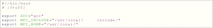
Set the environment variables. The Makefile in the main directory assumes that the C compiler can be called by using $(GCC), the MPI header file is found at $(MPI_INCLUDE)/mpi.h, the MPI compiled library is found in the $(MPI_HOME)/lib/ directory, and the mpicc command is available. The needed environment variables can be defined in the appropriate shell initialization files, e.g.
- 3.
Choose the intrinsics acceleration options. Some pieces of code exist in several versions: plain C, inline-assembly with SSE instructions, and inline-assembly with AVX instructions. The default Makefile uses the C version of the code. In order to use the inline-assembly version, one needs to modify the CFLAGS variable defined in lines 122–124 of main/Makefile. For instance, on some x86-64 machines one can use
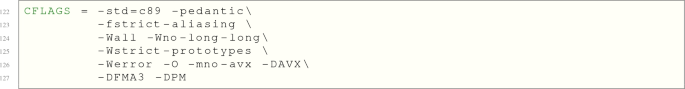
which activates AVX and FMA3 instructions and assumes that prefetch instructions fetch 64 bytes at a time. For a full description of available options, refer to the README file in the root directory.
- 4.
Choose the lattice geometry. The lattice geometry is chosen at compile time by modifying the macros defined in the first part of the include/global.h file. A full description of these macros can be found in the main/README.global file. For instance the following choice
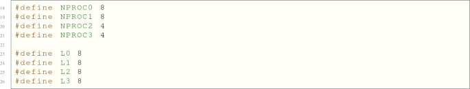
corresponds to an \(8^4\) local lattice, replicated on an \(8^2 \times 4^2\) MPI process grid (the code will need to be run with 1024 MPI processes), which yields a \(64^2 \times 32^2\) global lattice. As explained in Sect. 2.1, this choice of simulation parameters corresponds to a \(64^2 \times 32^2\) physical global lattice if no \(\mathrm {C}^*\) boundary conditions are used, or to a \(64 \times 32^3\) physical global lattice if \(\mathrm {C}^*\) boundary conditions are used in at least one spatial direction. In our implementation, NPROCn has to be a multiple of 2 if \(\mathrm {C}^*\) boundary conditions are used in the direction \(\texttt {n}=1,2,3\).
- 5.
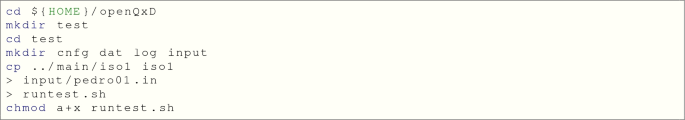
Compile the iso1 program and prepare for running. At this point, the code is ready to be compiled. Assuming that the root directory of the code is $HOME/openQxD, this is done by executing the following commands in a bash shell.

One can set up the directories and files to run the code by executing the following commands in a bash shell.
- 6.
Edit the input file. The input file input/pedro01.in must contain all adjustable parameters of the simulation (except the few ones that have been set at compile time). A rough guide on how to construct an input file for the iso1 program is found in Sect. 3.2.2. Alternatively, a sample input file can be cut and paste from Appendix C.
- 7.
Start the simulation. Edit the runtest.sh script as follows:

The runtest.sh script contains the command that invokes the iso1 program. It can be launched via a standard mpirun command, or incorporated in a script for a job scheduler. Recall that the number of needed MPI processes has been decided at compile time, and it is equal to 1024 in this case. The iso1 program takes a number of command-line options: the input file is specified with the -i option, the -noloc option specifies that the configuration files must be saved by a single MPI process, the -rmold specifies that only the most recent configuration must be kept and all previous ones must be deleted. The program will start the simulation from a randomly generated configuration. More details about the command-line options can be found in the main/README.iso1 file.
- 8.
Interrupt the simulation. Assuming that no error is produced, the simulation code will end naturally when all the configurations requested in the input file are generated. If the simulation needs to be interrupted earlier, one can just execute the following commands in a bash shell.

The simulation code will stop gracefully right after the next configuration is saved.
- 9.
Resume the simulation. Assuming that the last generated configuration was pedro01n42, edit the input file and set the nth variable in the [MD trajectories] section to 0 (see below for a description of the input file), and edit the runtest.sh script as follows:

Once this is executed, the simulation will continue from where it was interrupted.


3.2.2 Constructing the input file for iso1
Most of the parameters needed to generate configurations are passed to the iso1 program by means of a human-readable input file, in this case pedro01.in in the test/input directory. For a full description of the various parameters, the reader is referred to the main/README.iso1 and doc/parms.pdf files (and references therein). A rough guide to the various sections that compose the input file is provided here, with no ambition of completeness.
- 1.
Run name and output directories.
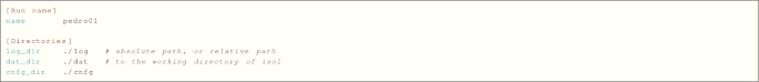
The program iso1 will produce several output files:
./log/pedro01.log, human-readable file, with general information about the simulation;
./dat/pedro01.dat, binary file, with the history of simple diagnostic observables;
./dat/pedro01.ms3.dat and ./dat/pedro01.ms5.dat, binary files, with the history of SU(3) and U(1) Wilson flow observables;
./dat/pedro01.par, binary file, with all simulation parameters;
./dat/pedro01.rng, binary file, with the state of the random number generator at the time of the most recent saved configuration;
./cnfg/pedro01n*, binary files, with the gauge configuration.
For every file in the log and dat directories, a backup file identified by a tilde at the end of its name is created and updated every time a configuration is saved.
- 2.
Schedule management.

The program iso1 will print one entry in the log file every 5 MD trajectories, will measure and print Wilson flow observables every 10 MD trajectories, will save a configuration every 50 MD trajectories. The first 100 trajectories are considered of thermalization (no observables are measured), a total of 800 MD trajectories will be generated and 15 configurations will be saved.
- 3.
Ranlux [45] initialization.

- 4.
Boundary conditions.

In this case periodic boundary conditions are chosen in time, and \(\mathrm {C}^*\) boundary conditions in all 3 spatial directions. The implementation of \(\mathrm {C}^*\) boundary conditions in openQ*D is described in Sect. 2.1. If SF or open-SF boundary conditions are chosen in time, the number of parameters in this section increases, as one needs to specify the value of the fields on the SF boundaries. For a full description of these parameters, refer to doc/parms.pdf.
- 5.
Gauge actions.
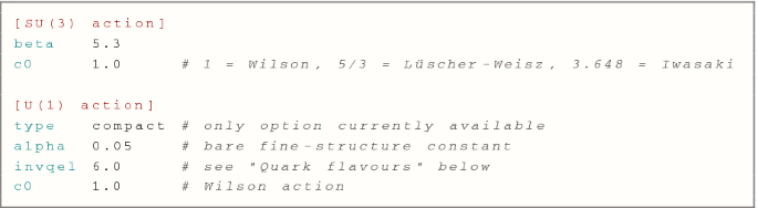
If different boundary conditions in time are chosen, the number of parameters in these sections increases, as one needs to specify the O(a)-improvement boundary coefficients. Refer to doc/gauge_action.pdf, doc/parms.pdf of all these parameters.
- 6.
Quark flavours. In the terminology of the openQ*D code, a quark flavour is identified by all adjustable parameters that define the Dirac operator. For instance, in a simulation in the isospin symmetric limit, the up and down quark count as a single quark flavour. In the following example, two quark flavours are requested, and the parameters of the corresponding Dirac operators are initialized.
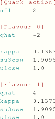
If different boundary conditions in time are chosen, the number of parameters in these sections increases, as one needs to specify the O(a)-improvement boundary coefficients. Also, if no \(\mathrm {C}^*\) boundary conditions are used, one can choose phase-periodic boundary conditions for fermions in space. Refer to doc/dirac.pdf, doc/parms.pdf for a detailed explanation of all these parameters.
- 7.
Rational approximation. With \(\mathrm {C}^*\) boundary conditions, the Pfaffian of the even–odd preconditioned Dirac operator \({\hat{D}}\) is needed, whose absolute value can be generated by a pseudofermion effective action of the type \(\psi ^\dag (\hat{D}^\dag \hat{D})^{-1/4} \psi \). The fractional power of \(\hat{D}^\dag \hat{D}\) is replaced by a rational approximation, which must be generated by means of the minmax program [46, 47]. We sketch here how to use this program, see minmax/README for more details.
First, one needs to modify the GCC and MPLIBPATH variables in minmax/Makefile. The Makefile assumes that the C compiler can be called by using $(GCC), the GMP and MPFR header files are found in the $(MPLIBPATH)/include/ directory, and the compiled libraries are found in the $(MPLIBPATH)/lib/ directory.

The minmax program is compiled and executed with the following commands in a bash shell.

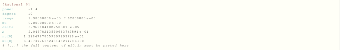
A rational approximation for \((\hat{D}^\dag \hat{D})^\alpha \) is requested, with \(\alpha =(-1)/(4)\) (-p and -q options), assuming that the eigenvalues of \((\hat{D}^\dag \hat{D})^{1/2}\) are in the interval \([1.98 \times 10^{-3} , 7.62]\) (-ra and -rb options), with a target relative precision of \(6 \times 10^{-5}\) (-goal option). The spectral range of \((\hat{D}^\dag \hat{D})^{1/2}\) must be guessed at first, but after some configurations have been generated it can be calculated with the program main/ms2. The minmax program creates a directory with a very long name, in this case
$$\begin{aligned}&\texttt {p-1q4mu0.00000000e+00ra1.98000000e}\\&\quad \texttt {-03rb7.62000000e+00} \end{aligned}$$which contains several files named n*.in. The integer in the file name corresponds to the order of the generated rational approximation. Only the highest order rational approximation, n10.in in this case, meets the requested precision. The full content of the n10.in must be pasted in the input file in a section of the following type,
Notice that more than one rational approximation can be used in the same input file (e.g. one may want to use different rational approximations for the up, down and strange quarks). Each rational approximation is identified by the integer in the section title.
- 8.
MD Hamiltonian and integrator.
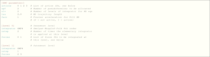
The MD Hamiltonian is given by the canonical kinetic term of the SU(3) gauge field, the kinetic term of the U(1) gauge field, and a sum of terms which do not depend on the MD momenta and are referred to as actions. The kinetic term of the U(1) gauge field can be chosen to be of two types: the canonical one (facc=0), or the Fourier-accelerated one (facc=1). Refer to doc/fourier.pdf and Sect. 2 for details on Fourier acceleration. The MD equations are solved by means of an approximate symplectic multilevel integrator, built in terms of standard elementary integrators. For each level, one needs to specify how many times the elementary integrator needs to be applied and which forces need to be integrated. Refer to doc/parms.pdf and module/update/README.mdint for details on the integrator.
The actions and forces are uniquely identified by an ID. Obviously there is a one-to-one correspondence between actions and forces. Corresponding actions and forces must share the same ID. The gauge actions and forces must be included, i.e.
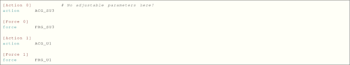
In this example, two pseudofermion actions are used (notice that this number matches the number of pseudofermion fields requested in the [HMC parameters] section), one for up quark and one for the down quark.
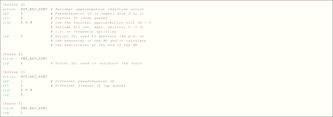
Notice that openQ*D allows for frequency splitting (not used in this example): the poles and zeroes of the rational approximations can be separated in different pseudofermion actions. This is convenient because one may want to integrate different poles and zeroes in different levels of the integrator, and also one may want to use different solvers for different poles. For details on the pseudofermion actions and forces, and on the frequency splitting, one should refer to doc/rhmc.pdf and Sect. 2.
- 9.
Solvers. Two multi-shift CG solvers are used in this example, with different residue for the actions and the forces.
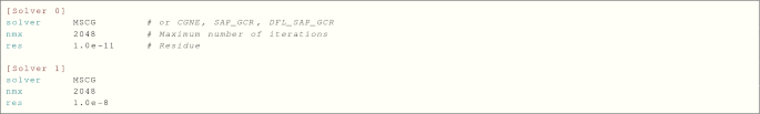
For details on the usage of other solvers, one should refer to doc/parms.pdf. The deflated solver (DFL_SAP_GCR) requires to set parameters for the generation and update of the deflation subspaces, also described in doc/parms.pdf. See also Sect. 4.4.
- 10.
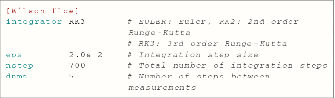
Wilson flow parameters. The iso1 program measures on the fly a number of simple observables (actions, SU(3) topological charge, electromagnetic fluxes) at positive flow time.


Results for strong (left) and weak (right) scaling of the application of the Dirac operator and SAP preconditioner as explained in the text. The speedup factors for the Dirac operator are multiplied by a factor 10 for better visibility. The dashed lines indicate perfect scaling behaviour accordingly
4 Performance and testing
4.1 Code performance on parallel machines
For future reference and comparison, benchmark measurements have been performed for the timing of the application of the double precision Wilson–Dirac operator and the SAP (Schwartz-Alternating-Procedure) preconditioner. The HPC cluster at CERN has been used, which features 72 nodes, each of them with two 8-core Intel® Xeon processors (E5-2630 v3, Haswell) running at about 2.4 GHz base frequency (3.6 GHz max.). Nodes are connected with Mellanox® Infiniband FDR (56 Gb/s).
The timings are obtained with the time2 programs located in the subdirectories devel/dirac and devel/sap. All measured times have been normalised to the smallest partition (one node or 16 cores). The results of these scaling tests are shown in Fig. 3. A QCD+QED setup with open boundary conditions in time and \(\mathrm {C}^*\) boundary conditions in one spatial direction has been used.
The weak scaling test has been performed with a local lattice size of \(8 \times 16 \times 8 \times 8\), giving an extended lattice with total volume  . Because of the \(\mathrm {C}^*\) boundary conditions this corresponds to a physical lattice with volume
  , cf. Sect. 2.1. While for the Dirac operator, parameters similar to the Quark flavours example (point 6) in Sect. 3.2 have been used, the SAP preconditioner specifically employs a block size of \(4^4\) with five SAP cycles (ncy 5) and five iterations (nmr 5) of the even–odd preconditioned Minimal Residue (MinRes) block solver. The setup is similar for the strong scaling study but with a constant total volume of \(V_{\mathrm {C}^*} =2 \cdot 64\times 32^3\) and varying local lattice sizes. In case of the double precision Wilson–Dirac operator, a much larger lattice volume with \(V_{\mathrm {C}^*} =2\cdot 64^4\) total lattice points was probed as well. As it can be seen in the left panel of Fig. 3 the larger lattice is performing even better than the smaller one.
In summary, the overall scaling studied here is close to optimal and small deviations may partly result from remaining indigestions of the underlying network. Similar studies have to be done on other machines but the overall behaviour is expected to be similar to the original openQCD code. Indeed, as already stressed, the openQ*D solvers are identical to the openQCD one. The Dirac operator is almost identical in the two codes, with the only difference that openQ*D uses the precalculated U(3) gauge field \(U z^{{\hat{q}}}\) instead of the SU(3) gauge field U. At fixed gauge background, the number of operations per lattice site performed by the Dirac operator is identical in the two codes, and so is the number of operations per lattice site per cycle performed by the solvers.
4.2 Low-level tests
The openQ*D code has been tested by means of an extensive battery of check programs, which can be found in the subdirectories of devel.Footnote 4 These programs have been taken over from openQCD-1.6 and NSPT-1.4, and extended in order to test the specific feature of the openQ*D code. Roughly speaking, the check programs in each devel subdirectory test features of the corresponding module subdirectory. Many check programs test also interactions between different modules. These programs are meant to be used by developers only and contain very limited documentation. Providing a description of the check programs is outside of the scope of this paper, and a short description can be found in the INDEX files in each devel subdirectory. However, it is worth to point out a few facts. All check programs have been run with all possible combinations of boundary conditions in the space and temporal directions. Whenever possible, all check programs have been run in a pure QCD setup (i.e. only the SU(3) gauge field is allocated), a pure QED setup (i.e. only the U(1) gauge field is allocated), and a QCD+QED setup (i.e. both gauge fields are allocated). All check programs have been run with various geometric configurations, i.e. lattice size and processor grid. Besides a plethora of minor details, specific check programs have been written to test:
the implementation of \(\mathrm {C}^*\) boundary conditions for both gauge fields and for the Dirac operator;
general properties of the Dirac operator with generic electric charge (e.g. gauge convariance, translational covariance, \(\gamma _5\)-hermiticity, comparison to analytic expression in case of zero gauge field);
the rational approximation of generic powers, and the associated reweighting factors;
the forces for the U(1) field, the QED action, the U(1) Wilson flow, the U(1) observables (e.g. clover field tensor, electromagnetic fluxes);
the MD with the U(1) field, with and without Fourier acceleration.

Violations of MD Hamiltonian conservation \(\Delta H\) as a function of the MD integration step-size \(\Delta \tau \), for all available integrators (LF, OMF2, OMF4), with and without Fourier Acceleration (FA). The lines represent the fit functions provided in the legend
4.3 Conservation of the Hamiltonian with Fourier acceleration
The use of Fourier Acceleration in QCD+QED simulations modifies the MD Hamiltonian and, consequently, the MD equations. In order to test the consistency between the two, one can look at the violation \(\Delta H\) of Hamiltonian conservation as a function of the MD integration step-size \(\Delta \tau \). The violation should vanish as a positive power of the integration step-size in the \(\Delta \tau \rightarrow 0\) limit. The power depends on the chosen integrator. When the total trajectory length is kept constant, the leap-frog integrator (LF) and 2nd order Omelyan–Mryglod–Folk (OMF2) integrators yield \(\Delta H \sim (\Delta \tau )^2\), while the 4th order Omelyan–Mryglod–Folk (OMF4) integrator yields \(\Delta H \sim (\Delta \tau )^4\).
Figure 4 shows the violation \(\Delta H\) as a function of \(\Delta \tau \) for all integrators, with and without Fourier Acceleration. A two parameter function \(\Delta H = a \, \Delta \tau ^b\) has been fitted to the data points. In all cases the obtained exponent is reasonably close to the expected one. This test has been performed on a single thermalized configuration taken from the Q*D1 ensemble (Table 1). As expected there is a clear hierarchy among the three integrators. More interestingly, Fourier Acceleration has the effect of reducing significantly \(\Delta H\). While no definite conclusion can be drawn from a single-configuration experiment in this regard, the same phenomenon has been observed in the generation of ensembles with the same parameters as the Q1 and Q2 runs described in [48], Table 2, with and without Fourier Acceleration: when Fourier Acceleration is turned on, if one wants to keep the acceptance rate the same, larger values of \(\Delta \tau \) can be typically chosen. Obviously this does not mean that it is always convenient to use Fourier Acceleration. In order to understand whether this is the case, one should take into account the computational overhead and the variation in autocorrelations. Fourier acceleration is known to reduce significantly autocorrelations in the case of the free scalar theory, but also in the case of non-compact pure U(1) theory [11], which is a theory of free photons. However, in the experiments with the Q1 and Q2 ensembles discussed above, no significant difference could be detected in the autocorrelation times after thermalization. This may indicate that autocorrelations are unaffected by Fourier Acceleration in the interacting case. Substantiating this statement certainly requires a much more detailed study.
4.4 Performance of locally deflated solver in QCD+QED

Mass of the \({\bar{Q}}' \gamma _5 Q\) valence pseudoscalar neutral meson has been calculated as a function of q and \(am_0=1/(2\kappa )-4\). QCD + qQED setup: SU(3) configurations are taken from the QCD1 ensemble (Table 1) and pure U(1) configurations are generated with \(\alpha _\mathrm {0}= 0.05\) and \(q_\text {el}=1/6\). The dashed curves are fits to the expected (leading order) quark mass dependence, \([m_{\mathrm {PS}}(q)]^2 = B(q) \{m_0-m_\mathrm {cr}(q)\}\), and are shown only to guide the eye. The gray dashed line indicates the mass of the unitary point of the QCD simulation. In all cases, 50 gauge configurations separated by 26 MDUs have been used
The use of efficient solvers is a key factor in enabling simulations at quark masses close to the physical point. The openQ*D code inherits all the solvers of the openQCD-1.6 package: Conjugate Gradient (CG), Multi-Shift Conjugate Gradient (MSCG), Generalized Conjugate Residual algorithm with Schwartz-Alternating-Procedure as preconditioning (SAP+GCR), and a deflated version of it (DFL+SAP+GCR). The deflated solver implements the idea of inexact deflation introduced in [22, 53] and an improvement involving inaccurate projection in the deflation preconditioner proposed in [54].
As the Dirac operator is passed as an argument to these solvers, their implementation is blind to the coupling to the U(1) field and to \(\mathrm {C}^*\) boundary conditions. The efficiency of these solvers may be affected in principle by the coupling to the U(1) field, i.e. may depend on the electric charge of the Dirac operator. However this turns out not to be the case. The goal of this section is to describe two tests in support of this statement. These tests have been run on Altamira HPC at IFCA-CSIC, which consists of 158 computing nodes, each of them with two Intel® Xeon processors (E5-2670) at 2.6 GHz. Nodes are connected with Mellanox® Infiniband FDR (56 Gb/s).
An electroquenched (QCD+qQED) setup has been considered for both tests, with SU(3) configurations from the QCD1 ensemble (Table 1) and pure U(1) configurations generated with \(\alpha _\mathrm {0}= 0.05\) and \(q_\mathrm {el}=1/6\). Two degenerate valence quarks Q and \(Q'\) have been considered, with electric charge q and bare mass \(m_0\). The mass \(m_{\mathrm {PS}}\) of the \({\bar{Q}}' \gamma _5 Q\) valence pseudoscalar neutral meson has been calculated as a function of q and \(m_0\) and is shown in Fig. 5. Notice that the critical bare mass depends very heavily on the electric charge, as expected. For this reason it makes sense to compare the solver performance for different electric charges keeping fixed the value of \(m_{\mathrm {PS}}\) (rather than the bare mass).
In the first test, the time needed to invert the even–odd preconditioned Dirac operator (with a representative QCD+qQED configuration) on 15 random sources has been measured, using the CG, SAP+GCR, and DFL+SAP+GCR solvers. The shortest time has been plotted in Fig. 6 for electric charges \(q=0,-1/3,2/3\) and a range of values of \(m_{\mathrm {PS}}\). It is evident that the performance of all solvers is insensitive to the electric charge.

Comparison of performance of various solvers and various electric charges as a function of the mass \(m_{\mathrm {PS}}\) of the valence neutral pion. In all cases, the inverse of the even–odd preconditioned Dirac operator has been calculated on random sources. One representative QCD+qQED configuration has been used (SU(3) configuration from the QCD1 ensemble, Table 1, and pure U(1) configuration generated with \(\alpha _\mathrm {0}= 0.05\) and \(q_\mathrm {el}=1/6\)). The same residue of \(10^{-10}\) has been chosen for the three solvers. The solver performance is insensitive to the electric charge

Comparison of performance of various solvers and various electric charges as a function of the twisted mass \(\mu \). In all cases, the inverse of \((\hat{D}^\dag \hat{D}+ \mu ^2)\) has been calculated on random sources. The mass of the valence neutral pion (calculated at \(\mu =0\)) has been chosen to be \(m_{\mathrm {PS}}\simeq 329\,\mathrm {MeV}\). One representative QCD+qQED configuration has been used (SU(3) configuration from the QCD1 ensemble, Table 1, and pure U(1) configuration generated with \(\alpha _\mathrm {0}= 0.05\) and \(q_\mathrm {el}=1/6\)). The same residue of \(10^{-8}\) has been chosen for the three solvers. The solver performance is insensitive to the electric charge. As expected, the deflated solver loses efficiency at large values of \(\mu \) and eventually fails to converge for the three highest value
One important caveat needs to be pointed out for the DFL+SAP+GCR solver. Before applying this solver, one needs to generate the deflation subspace, which is constructed from approximate eigenvectors of the Dirac operator. The code allows the possibility to choose different parameters for the Dirac operator used in the solver and the one used to generate the deflation subspace. This is very useful in practice since having a slightly heavier bare mass or even a twisted mass for the generation of the deflation subspace generally speeds up the calculation without affecting the performance of the solver. On the other hand, it is crucial to generate the deflation subspace with the same electric charge of the Dirac operator that needs to be inverted. If this is not done, the DFL+SAP+GCR solver loses efficiency dramatically. For this reason, in contrast to openQCD-1.6, the openQ*D code can handle simultaneously several deflation subspaces. These deflation subspaces can be generated with different parameters and will all be updated during the MD evolution. The user can specify in the input file which deflation subspace should be used for each DFL+SAP+GCR solver independently. In practice, in a realistic QCD+QED simulation, one would need to generate only two deflation subspaces, one for up-type quarks and one for down-type quarks. It has been checked also that the time needed to generate the deflation subspace is insensitive to the electric charge as long as \(m_{\mathrm {PS}}\) is kept fixed.
In the second test, a single value of \(m_{\mathrm {PS}}\simeq 354\,\mathrm {MeV}\) has been chosen, and the time needed to invert \((\hat{D}^\dag \hat{D}+\mu ^2)\) has been measured for various values of the twisted mass \(\mu \), using the CG and DFL+SAP+GCR solvers. One representative QCD+qQED configuration and 48 random sources have been used. The shortest time has been plotted in Fig. 7 for electric charges \(q=0,-1/3,2/3\) and a range of values of \(\mu \). The inversion of \((\hat{D}^\dag \hat{D}+ \mu ^2)\) is relevant to calculate the rational approximation of non-integer powers of \(\hat{D}^\dag \hat{D}\) (see Sect. 2). Also in this case, the performance of the two solvers is seen to be insensitive to the electric charge as long as \(m_{\mathrm {PS}}\) is kept fixed.

Selected observables for simulation Q*D1 including thermalisation part. Left–right/top–bottom: HMC energy violations \(\Delta H\), average plaquette for SU(3) and U(1) gauge fields, energy density E(t) for SU(3), energy density for U(1), topological charge Q(t), lowest eigenvalue \({\hat{\lambda }}_\mathrm{min}\) in the spectrum of \(|\gamma _5 \hat{D}|\), and reweighting factors \(W_q\) for two different numerical accuracies, \(\delta =O(10^{-11})\) (left) and \(\delta =O(10^{-9})\) (right)
4.5 Key observables for HMC simulations of QCD\(+\)QED
Beside the electroquenched tests in the previous section, a new set of tests is done using dynamical QCD+QED simulations with Wilson fermions and \(\mathrm {C}^*\) boundary conditions. The dynamical degrees of freedom of the U(1) gauge field are included in the simulation labeled Q*D1 in Table 1. Q*D1 takes over the parameters from the H200 ensemble of the \(N_\mathrm {f}=2+1\) CLS [55] effort, except that the lattice extent is halved in each of the space-time directions. As the dynamical U(1) degrees of freedom contribute to the renormalization of the bare parameters, the estimate for the lattice spacing and pion mass cannot be taken over from the CLS ensembles,Footnote 5 but rather need to be estimated independently. Such an endeavour is beyond the scope of this paper. However, an estimate for \(t_0/a^2\) is given in Table 1 for future reference. The reference flow time \(t_0\) is implicitly given by \([t_0^2\langle E(t_0)\rangle ]=0.3\) using the Wilson flow and clover discretisation of the SU(3) field strength tensor in the definition of the energy density E(t) [56]. A rough estimate of a is given after naively matching \(t_0/a^2\) to the data provided in Table III of Ref. [52].
Although openQ*D allows for twisted-mass reweighting, that option is not required for Q*D1 (\({\mu }=0.0\)). All three bare sea quark masses, \(am_{0,i}=1/(2\kappa _i)-4\), are taken to be degenerate. As demonstrated in the previous section and shown in Fig. 5, this necessarily leads to a large difference in the neutral pseudoscalar masses due to the differences in quark charges. One thus ends up with a degenerate pair of down-type quarks (\(q=-1/3\)), and a single but significantly heavier up-type quark (\(q=2/3\)). Hence, the simulations are essentially probing a somewhat unphysical version of the \(N_\mathrm {f}=2+1\) theory, but are sufficient to probe standard observables and performance of the code.
In Fig. 8 a summary of selected observables is given for simulation Q*D1. The run was stable and did not show any particular issue during the course of the simulation. Most of the observables presented in the following include the thermalisation part. Starting from a random configuration, the HMC energy violations, measured every trajectory (\(\tau =0.7\) MDU), drop after a few iterations and stably fluctuate in the range \([-\,0.5,+\,0.5]\). The simulation employs the OMF4 integrator without Fourier acceleration and the spectral ranges of the individual quark flavours have been properly set. Next the average plaquette for the SU(3) and U(1) gauge fields are presented. The former is shifted by a constant amount for better comparison. The SU(3) plaquette has much larger statistical fluctuations and requires longer thermalisation times than the U(1) plaquette even without Fourier acceleration. The next two plots show the two available definitions of the (renormalized) energy density E(t) at a flow time \(t=3.2\) for the SU(3) and U(1) part, respectively. The topological charge Q (measured at the same flow time) fluctuates well after rapid changes during the thermalisation phase of the run. The smallest eigenvalues of \(|\gamma _5 \hat{D}_\mathrm {u}|\) and \(|\gamma _5 \hat{D}_\mathrm {d/s}|\) follow, confirming that the lower end of the spectral ranges of the rational approximations have been chosen correctly. No exceptionally small values are present, which is not surprising considering the heavy pseudoscalar mass simulated here.
The Q*D1 run has been produced with a rational approximation with relative precision \(\delta = O(10^{-11})\). A second run has been performed with the same parameters as Q*D1 except for the rational approximation, which has been chosen with relative precision \(\delta = O(10^{-9})\). The logarithms of the reweighing factors for both runs are shown in the last two panes of Fig. 8. As expected, the reweighting factor for the run with a better rational approximation is closer to 1 (and its logarithm is closer to 0).
5 Summary and outlook
We presented openQ*D [1], the first open source package which allows to perform full lattice simulations of QCD+QED, QCD or QED. The code implements the proposal of Ref. [18] and allows to choose \(\mathrm {C}^*\) boundary conditions along the spatial directions but also periodic boundary conditions can be simulated efficiently. Moreover, the chosen theory can be simulated by choosing either periodic, Schrödinger Functional or open boundary conditions along the time direction.
The new code is based on the openQCD [2] package from which it inherits the highly optimized implementation of the Dirac operator, of the solvers, of the HMC and of the RHMC algorithms. The openQ*D package extends the algorithmic functionalities of the openQCD code by giving the possibility of using multiple deflation subspaces in a single simulation, of implementing rational approximations of generic powers of the Dirac operator (with and without twisted-mass preconditioning) and by implementing Fourier Acceleration for the evolution of the U(1) field.
We presented the main functionalities of the code and discussed the theoretical motivations behind the algorithmic choices and their specific implementations. We also presented a guide to instruct the user to run a full QCD+QED simulation with openQ*D and discussed the results of some tests. These include low-level tests aiming at assessing the correctness of the implementation of the different algorithms but also some benchmarks to measure the performance of the code.
In future releases we plan to add a number of features. Concerning the configuration generation, we will include the possibility to use a gauge-fixed non-compact formulation of QED. We will also provide programs to calculate a number of observables, in particular charged-meson two-point functions with QED dressing-factors along the lines of [18], and quark gradient flow observables [57]. Finally we will consider incorporating some of the algorithmic developments discussed in [58], in particular stabilized Wilson fermions.
Given the good performance and high scalability on modern supercomputing cluster architectures, openQ*D can profitably be used to generate QCD+QED gauge configurations with \(\mathrm {C}^*\) boundary conditions (but not only) in a realistic setup with the aim of computing QED radiative corrections to phenomenologically relevant observables.
Data Availability Statement
This manuscript has associated data in a data repository. [Authors’ comment: All presented data sets can be easily generated using openQ*D [1].]
Notes
The code allows also for (inefficient) simulations of QED in isolation, even though a main program for this purpose is not provided in the 1.0 version.
In the input file of a typical main program in openQ*D (see Sect. 3.2), one can choose the number of spatial directions with \(\mathrm {C}^*\) boundary conditions. \(\mathrm {C}^*\) boundary conditions are turned on sequentially in directions 1, 2 and 3.
The devel directory contains 46,224 lines of code, against 60,203 lines of code in the module directory.
Had the U(1) d.o.f. been switched off (\(\alpha _\mathrm {0}= 0\)), the chosen parameter set would correspond to \(a\approx 0.064\,\mathrm {fm}\) and \(m_{\mathrm {PS}}\approx 420\,\mathrm {MeV}\).
References
(RC*), I. Campos, P. Fritzsch, M. Hansen, M. Krstić Marinković, A. Patella, A. Ramos et al., “openQ*D.” GitLab: https://gitlab.com/rcstar/openQxD. CSIC: https://dx.doi.org/10.20350/digitalCSIC/8591. https://hdl.handle.net/10261/173334 (2019)
Simulation program for lattice QCD (openQCD code) (2016). https://cern.ch/luscher/openQCD
Numerical Stochastic Perturbation Theory (NSPT code) (2017). https://cern.ch/luscher/NSPT
(Flavour Lattice Averaging Group), S. Aoki et al., FLAG Review (2019). arXiv:1902.08191
V. Cirigliano, G. Ecker, H. Neufeld, A. Pich, J. Portoles, Kaon decays in the standard model. Rev. Mod. Phys. 84, 399 (2012). arXiv:1107.6001
D. Giusti, V. Lubicz, G. Martinelli, C.T. Sachrajda, F. Sanfilippo, S. Simula et al., First lattice calculation of the QED corrections to leptonic decay rates. Phys. Rev. Lett. 120, 072001 (2018). arXiv:1711.06537
M. Di Carlo, D. Giusti, V. Lubicz, G. Martinelli, C.T. Sachrajda, F. Sanfilippo et al., Light-meson leptonic decay rates in lattice QCD+QED. arXiv:1904.08731
(HFLAV), Heavy Flavor Averaging Group. https://hflav.web.cern.ch
S. de Boer, T. Kitahara, I. Nisandzic, Soft-photon corrections to \(\bar{B} \rightarrow D \tau ^{-} \bar{\nu }_{\tau }\) Relative to \(\bar{B} \rightarrow D \mu ^{-} \bar{\nu }_{\mu }\). Phys. Rev. Lett. 120, 261804 (2018). arXiv:1803.05881
S. Calí, S. Klaver, M. Rotondo, B. Sciascia, Impacts of radiative corrections on measurements of lepton flavour universality in \(B \rightarrow D \ell \nu _{\ell }\) decays. arXiv:1905.02702
S. Borsanyi et al., Ab initio calculation of the neutron–proton mass difference. Science 347, 1452–1455 (2015). arXiv:1406.4088
R. Horsley et al., Isospin splittings of meson and baryon masses from three-flavor lattice QCD + QED. J. Phys. G 43, 10LT02 (2016). arXiv:1508.06401
R. Horsley et al., QED effects in the pseudoscalar meson sector. JHEP 04, 093 (2016). arXiv:1509.00799
A. Patella, QED corrections to hadronic observables. PoS LATTICE2016, 020 (2017). arXiv:1702.03857
D. Bernecker, H.B. Meyer, Vector correlators in lattice QCD: methods and applications. Eur. Phys. J. A 47, 148 (2011). arXiv:1107.4388
T. Blum, N. Christ, M. Hayakawa, T. Izubuchi, L. Jin, C. Jung et al., Using infinite volume, continuum QED and lattice QCD for the hadronic light-by-light contribution to the muon anomalous magnetic moment. Phys. Rev. D 96, 034515 (2017). arXiv:1705.01067
X. Feng, L. Jin, QED self energies from lattice QCD without power-law finite-volume errors. arXiv:1812.09817
B. Lucini, A. Patella, A. Ramos, N. Tantalo, Charged hadrons in local finite-volume QED+QCD with C* boundary conditions. JHEP 02, 076 (2016). arXiv:1509.01636
P.A.M. Dirac, Gauge invariant formulation of quantum electrodynamics. Can. J. Phys. 33, 650 (1955)
(RC*), M. Hansen, B. Lucini, A. Patella, N. Tantalo, Gauge invariant determination of charged hadron masses. JHEP 05, 146 (2018). arXiv:1802.05474
G.M. de Divitiis, R. Frezzotti, V. Lubicz, G. Martinelli, R. Petronzio, G.C. Rossi et al., Leading isospin breaking effects on the lattice. Phys. Rev. D 87, 114505 (2013). arXiv:1303.4896
M. Lüscher, Deflation acceleration of lattice QCD simulations. JHEP 12, 011 (2007). arXiv:0710.5417
G.G. Batrouni, G.R. Katz, A.S. Kronfeld, G.P. Lepage, B. Svetitsky, K.G. Wilson, Langevin simulations of lattice field theories. Phys. Rev. D 32, 2736 (1985)
S. Duane, B.J. Pendleton, Gauge invariant fourier acceleration. Phys. Lett. B 206, 101–106 (1988)
M. Dalla Brida, M. Lüscher, SMD-based numerical stochastic perturbation theory. Eur. Phys. J. C 77, 308 (2017). arXiv:1703.04396
M. Lüscher, S. Schaefer, Lattice QCD with open boundary conditions and twisted-mass reweighting. Comput. Phys. Commun. 184, 519–528 (2013). arXiv:1206.2809
M. Lüscher, R. Narayanan, P. Weisz, U. Wolff, The Schrödinger functional: a renormalizable probe for nonAbelian gauge theories. Nucl. Phys. B 384, 168–228 (1992). arXiv:9207009
S. Sint, On the Schrödinger functional in QCD. Nucl. Phys. B 421, 135–158 (1994). arXiv:9312079
M. Lüscher, Step scaling and the Yang–Mills gradient flow. JHEP 06, 105 (2014). arXiv:1404.5930
A.S. Kronfeld, U.J. Wiese, SU(N) gauge theories with C periodic boundary conditions. 1. Topological structure. Nucl. Phys. B 357, 521–533 (1991)
A.S. Kronfeld, U.J. Wiese, SU(N) gauge theories with C periodic boundary conditions. 2. Small volume dynamics. Nucl. Phys. B 401, 190–205 (1993). arXiv:9210008
U.J. Wiese, C periodic and G periodic QCD at finite temperature. Nucl. Phys. B 375, 45–66 (1992)
L. Polley, Boundaries for SU(3)\({}_{C}\times \)U(1)\({}_{el}\) lattice gauge theory with a chemical potential. Z. Phys. C 59, 105–108 (1993)
I. Montvay, Supersymmetric Yang–Mills theory on the lattice. Int. J. Mod. Phys. A 17, 2377–2412 (2002). arXiv:0112007
S. Ali, G. Bergner, H. Gerber, P. Giudice, I. Montvay, G. Münster et al., The light bound states of \(\cal{N}=1\) supersymmetric SU(3) Yang–Mills theory on the lattice. JHEP 03, 113 (2018). arXiv:1801.08062
T.A. DeGrand, A conditioning technique for matrix inversion for Wilson Fermions. Comput. Phys. Commun. 52, 161–164 (1988)
A.D. Kennedy, I. Horvath, S. Sint, A New exact method for dynamical fermion computations with nonlocal actions. Nucl. Phys. Proc. Suppl. 73, 834–836 (1999). arXiv:9809092 ([,834(1998)])
M. Lüscher, F. Palombi, Fluctuations and reweighting of the quark determinant on large lattices. PoS LATTICE2008, 049 (2008). arXiv:0810.0946
J.C. Sexton, D.H. Weingarten, Hamiltonian evolution for the hybrid Monte Carlo algorithm. Nucl. Phys. B 380, 665–677 (1992)
I. Omelyan, I. Mryglod, R. Folk, Symplectic analytically integrable decomposition algorithms: classification, derivation, and application to molecular dynamics, quantum and celestial mechanics simulations. Comput. Phys. Commun. 151, 272–314 (2003)
I. Campos, P. Fritzsch, M. Hansen, M.K. Marinković, A. Patella, A. Ramos et al., openQ*D simulation code for QCD + QED. EPJ Web Conf. 175, 09005 (2018). arXiv:1710.08839
(RC*), “openQ*D documentation, Gauge actions,doc/gauge\_action.pdf.”
(RC*), “openQ*D documentation, Dirac operator, doc/dirac.pdf.”
M. Lüscher, S. Sint, R. Sommer, P. Weisz, Chiral symmetry and O(a) improvement in lattice QCD. Nucl. Phys. B 478, 365–400 (1996). arXiv:9605038
M. Lüscher, A portable high quality random number generator for lattice field theory simulations. Comput. Phys. Commun. 79, 100–110 (1994). arXiv:9309020
E. Remes, Sur le calcul effectif des polynômes d’approximation de Tchebichef. C. R. Acad. Sci. Paris 199, 337–340 (1934)
A. Ralston, Rational Chebyshev approximation by Remes’ algorithms. Numerische Mathematik 7, 322–330 (1965)
M. Hansen, B. Lucini, A. Patella, N. Tantalo, Simulations of QCD and QED with C* boundary conditions. EPJ Web Conf. 175, 09001 (2018). arXiv:1710.08838
J. Bulava, S. Schaefer, Improvement of \(N_f=3\) lattice QCD with Wilson fermions and tree-level improved gauge action. Nucl. Phys. B 874, 188–197 (2013). arXiv:1304.7093
(ALPHA), K. Jansen, R. Sommer, O(a) improvement of lattice QCD with two flavors of Wilson quarks. Nucl. Phys. B 530, 185–203 (1998). arXiv:9803017. (Erratum: Nucl. Phys.B643,517(2002))
P. Fritzsch, F. Knechtli, B. Leder, M. Marinkovic, S. Schaefer, R. Sommer et al., The strange quark mass and Lambda parameter of two flavor QCD. Nucl. Phys. B 865, 397–429 (2012). arXiv:1205.5380
M. Bruno, T. Korzec, S. Schaefer, Setting the scale for the CLS \(2 + 1\) flavor ensembles. Phys. Rev. D 95, 074504 (2017). arXiv:1608.08900
M. Lüscher, Local coherence and deflation of the low quark modes in lattice QCD. JHEP 07, 081 (2007). arXiv:0706.2298
A. Frommer, K. Kahl, S. Krieg, B. Leder, M. Rottmann, Adaptive aggregation based domain decomposition multigrid for the lattice Wilson Dirac operator. SIAM J. Sci. Comput. 36, A1581–A1608 (2014). arXiv:1303.1377
M. Bruno et al., Simulation of QCD with \(N_f=2+1\) flavors of non-perturbatively improved Wilson fermions. JHEP 02, 043 (2015). arXiv:1411.3982
M. Lüscher, Properties and uses of the Wilson flow in lattice QCD. JHEP 08, 071 (2010). arXiv:1006.4518 (Erratum: JHEP03,092(2014))
M. Lüscher, Chiral symmetry and the Yang-Mills gradient flow. JHEP 04, 123 (2013). arXiv:1302.5246
A. Francis, P. Fritzsch, M. Lüscher, A. Rago, Master-field simulations of O(a)-improved lattice QCD: algorithms, stability and exactness. arXiv:1911.04533
M. Hasenbusch, Speeding up the hybrid Monte Carlo algorithm for dynamical fermions. Phys. Lett. B 519, 177–182 (2001). arXiv:0107019
Acknowledgements
The simulations were performed on the following HPC systems: Altamira, provided by IFCA at the University of Cantabria; FinisTerrae II, provided by CESGA (Galicia Supercomputing Centre); the Lonsdale cluster maintained by the Trinity Centre for High Performance Computing; and the Lattice-HPC cluster at CERN. FinisTerrae II was funded by the Xunta de Galicia and the Spanish MINECO under the 2007–2013 Spanish ERDF. Lonsdale was funded through grants from the Science Foundation Ireland. We thankfully acknowledge the computer resources offered and the technical support provided by the staff of these computing centers. We thank the Theoretical Physics Department at CERN for hospitality during the workshop Advances in Lattice Gauge Theory 2019, allowing us to jointly finalise the present work.
Author information
Authors and Affiliations
Corresponding author
Appendices
Implementation of the RHMC
1.1 Rational approximation
It is convenient to introduce the hermitian operator \({\hat{Q}}=\gamma _5 {\hat{D}}\), in terms of which \({\hat{D}}^\dag {\hat{D}} = {\hat{Q}}^2\). Assume that the spectrum of \(|{\hat{Q}}|\) is contained in the interval \([r_a,r_b]\), and choose an integer n. A rational function of order [n, n] in \(q^2\) has the form
Without loss of generality one can assume
\(\rho (q^2)\) is chosen to be the optimal rational approximation of order [n, n] of the function \((q^2 + {\hat{\mu }}^2)^{-\alpha }\) in the domain \(q \in [r_a,r_b]\), i.e. the rational function of the form (A.1) which minimizes the uniform relative error
As explained in Sect. 3.2.2, the optimal rational approximation can be calculated with the minmax code which implements the minmax approximation algorithm in multiple precision.
If \(\rho (q^2)\) is the desired optimal rational approximation, the operator \(R\) which appears in Eq. (2.6) is defined simply as
Equation (A.3) implies the following norm bound
1.2 Frequency splitting and pseudofermion action
openQ*D inherits from openQCD the frequency splitting of the rational approximation: the factors of the rational approximation can be split in different pseudofermion actions; the corresponding forces can be included in different levels of the MD integrator, providing a useful handle to optimize the algorithm. This procedure is similar to the Hasenbusch decomposition for the HMC algorithm [59].
The rational approximation constructed in Sect. A.1 is broken up in factors of the form
For example, if \(n = 12\) a possible factorization is
The contribution of \(R\) to the quark determinant is
Each \(P_{k,l}^{-1}\) determinant is simulated as usual by adding a pseudofermion action of the form
where the fields \(\phi ^{k,l}_\text {e}\) are independent pseudofermions that live on the even sites of the lattice. By using a partial fraction decomposition
the pseudofermion action in Eq. (A.9) is cast into a sum of terms of the type
1.3 Reweighting factors
Let \(\tilde{R}\) and \(R\) be the optimal rational approximations of order [n, n] for \(({\hat{D}}^\dag {\hat{D}})^{-\alpha }\) and \(({\hat{D}}^\dag {\hat{D}} + {\hat{\mu }}^2)^{-\alpha }\) respectively. It is assumed that the relative errors of the two rational approximations are not greater than \(\delta \) in the common spectral range \([r_a,r_b]\).
The reweighting factor W defined in Eq. (2.8) is decomposed in two factors which are calculated separately, i.e.
1.3.1 Reweighting factor \(W_\text {rat}\)
In the calculation of the reweighting factor \(W_\text {rat}\) in Eq. (A.14), it is assumed that the exponent \(\alpha \) is a positive rational number of the form
where u and v are natural numbers. The reweighting factor can be represented as
where the operator Z is defined as
The determinant in Eq. (A.17) is estimated stochastically
where the fields \(\eta ^j_\text {e}\) are N independent normally-distributed pseudofermions that live on the even sites of the lattice. From the norm bound in Eq. (A.5) for \({\hat{\mu }}=0\), and the positivity of \(\tilde{R}\) (which is guaranteed if the relative error \(\delta \) is small enough), it follows that
which yields the norm bound
Therefore the Taylor series
converges rapidly in operator norm. The exponent in Eq. (A.19) can be estimated from the first few terms of
It is possible to estimate the size of these terms by noting that \(\Vert \eta ^j_\text {e} \Vert ^2\) is very nearly equal to 12 times the number \(N_\text {e}\) of even lattice points. Taking the bound (A.21) into account, the following estimate is obtained
The statistical fluctuations of the exponents in Eq. (A.19) derive from those of the gauge field and those of the random sources \(\eta ^j_\text {e}\). For a given gauge field, the variance of the exponent is equal to
These fluctuations are guaranteed to be small if, for instance, \(12 N_\text {e} \delta ^2 \le 10^{-4}\). One can then just as well set \(N = 1\) in Eq. (A.19), i.e. a sufficiently accurate stochastic estimate of \(W_\text {rat}\) is obtained in this case with a single random source.
When the stronger constraint \(12 N_\text {e} \delta \le 10^{-2}\) is satisfied, the reweighting factor \(W_\text {rat}\) deviates from 1 by at most 1%. Larger approximation errors can however be tolerated in practice as long as the fluctuations of \(W_\text {rat}\) remain small.
1.3.2 Reweighting factor \(W_\mathrm{{rtm}}\)
Let us choose a rational approximation \(R\) of order [n, n] for \(({\hat{D}}^\dag {\hat{D}} + {\hat{\mu }}^2)^{-\alpha }\) of the form
and a rational approximation \(\tilde{R}\) of order [n, n] for \(({\hat{D}}^\dag {\hat{D}})^{-\alpha }\) of the form
Let us rewrite Eq. (A.15) as
Notice that the operator \(R^{-1} \tilde{R}\) is also a rational function of \({\hat{Q}}^2={\hat{D}}^\dag {\hat{D}}\). It is convenient to break up this rational function in factors of the type
If \(n = 12\), for example, the reweighting factor \(W_\text {rtm}\) can be factorized as
Each of the above determinants is estimated stochastically
where the fields \(\eta ^j_\text {e}\) are N independent normally-distributed pseudofermions that live on the even sites of the lattice. It is useful to consider the partial fraction decomposition
Typically \(\sigma _j\) and \({\tilde{\sigma }}_j\) are found to have opposite signs. Also, for small values of j, \(|\sigma _j|\) and \(|{\tilde{\sigma }}_j|\) are of the same order of magnitude, therefore it is convenient for numerical stability to use the following representation
Laplacian for the Fourier accelerated molecular dynamics
The U(1) momentum is generally represented in momentum space as
The basis functions \(e_\mu (p_0,x_0)\) (for fixed \(\mu \)) are orthogonal with respect to a weighted scalar product
where the weight \(w_\mu (x)\) is taken to be 1/2 if x belongs to an open boundary (i.e. \(x_0=0\) for open and open-SF b.c.s, and \(x_0=T-1\) for open b.c.s) and \(\mu =1,2,3\). In all other cases \(w_\mu (x)\) is taken to be 1. The relation between \(\pi \) and \({\tilde{\pi }}\) is easily inverted
The set \({\mathcal {P}}\) is given by all spatial momenta \(\mathbf {p} = (p_1,p_2,p_3)\) of the form
where \(c_k=0\) if k is a periodic direction and \(c_k=1\) if k is a \(\mathrm {C}^*\) direction. The sets \(E_\mu \) and the eigenfunctions \(e_\mu (p_0,x_0)\) depend on the boundary conditions in time. In the following \(k=1,2,3\).
Open boundary conditions:
$$\begin{aligned} E_0= & {} \frac{\pi }{N_0-1} \{ 1 , \dots , N_0-1 \}, \nonumber \\ E_k= & {} \frac{\pi }{N_0-1} \{ 0 , \dots , N_0-1 \}, \end{aligned}$$(B.5)$$\begin{aligned} e_0(p_0,x_0)= & {} \frac{i}{(1+\delta _{p_0,\pi })(N_0-1)} \sin \left[ p_0\left( x_0 + \frac{1}{2} \right) \right] ,\nonumber \\ \end{aligned}$$(B.6)$$\begin{aligned} e_k(p_0,x_0)= & {} \frac{1}{(1+\delta _{p_0,0}+\delta _{p_0,\pi })(N_0-1)} \cos ( p_0 x_0 ).\nonumber \\ \end{aligned}$$(B.7)SF boundary conditions:
$$\begin{aligned} E_0= & {} \frac{\pi }{N_0} \{ 0 , \dots , N_0-1 \}, \nonumber \\ E_k= & {} \frac{\pi }{N_0} \{ 1 , \dots , N_0-1 \}, \end{aligned}$$(B.8)$$\begin{aligned} e_0(p_0,x_0)= & {} \frac{1}{(1+\delta _{p_0,\pi })N_0} \cos \left[ p_0\left( x_0 + \frac{1}{2} \right) \right] ,\nonumber \\ \end{aligned}$$(B.9)$$\begin{aligned} e_k(p_0,x_0)= & {} \frac{i}{N_0} \sin ( p_0 x_0 ). \end{aligned}$$(B.10)Open-SF boundary conditions:
$$\begin{aligned} E_0= & {} E_k = \frac{\pi }{N_0} \left( \{ 0 , \dots , N_0-1 \} + \frac{1}{2} \right) ,\nonumber \\ \end{aligned}$$(B.11)$$\begin{aligned} e_0(p_0,x_0)= & {} \frac{i}{N_0} \sin \left[ p_0\left( x_0 + \frac{1}{2} \right) \right] , \end{aligned}$$(B.12)$$\begin{aligned} e_k(p_0,x_0)= & {} \frac{1}{N_0} \cos \left[ p_0\left( x_0 + \frac{1}{2} \right) \right] . \end{aligned}$$(B.13)Periodic boundary conditions:
$$\begin{aligned} E_0= & {} E_k = \frac{2\pi }{N_0} \{ 0 , \dots , N_0-1 \}, \end{aligned}$$(B.14)$$\begin{aligned} e_0(p_0,x_0)= & {} e_k(p_0,x_0) = \frac{1}{N_0} \exp ( i p_0 x_0 ). \end{aligned}$$(B.15)
We use the Fourier decomposition to define the intermediate operator \(D_\text {N}\)
Explicity
With respect to the scalar product defined by
the operator \(D_\text {N}\) is symmetric and strictly positive, i.e.
The desired operator is defined as
Symmetry and strict positivity of \(\Delta \) with respect to the canonical scalar product of \(\Delta \) follow from the corresponding properties of \(D_\text {N}\). Notice that
The openQ*D code uses the Fast Fourier Transform (FFT) algorithm to construct \({\tilde{\pi }}(p,\mu )\) from \(\pi (x,\mu )\) and vice versa. The FFT is implemented in the module dft which is an adaptation of the corresponding module in the NSPT-1.4 code written by Mattia Dalla Brida and Martin Lüscher [25].
Sample input file


Rights and permissions
Open Access This article is licensed under a Creative Commons Attribution 4.0 International License, which permits use, sharing, adaptation, distribution and reproduction in any medium or format, as long as you give appropriate credit to the original author(s) and the source, provide a link to the Creative Commons licence, and indicate if changes were made. The images or other third party material in this article are included in the article’s Creative Commons licence, unless indicated otherwise in a credit line to the material. If material is not included in the article’s Creative Commons licence and your intended use is not permitted by statutory regulation or exceeds the permitted use, you will need to obtain permission directly from the copyright holder. To view a copy of this licence, visit http://creativecommons.org/licenses/by/4.0/.
Funded by SCOAP3
About this article

Cite this article
Campos, I., Fritzsch, P., Hansen, M. et al. openQ*D code: a versatile tool for QCD+QED simulations. Eur. Phys. J. C 80, 195 (2020). https://doi.org/10.1140/epjc/s10052-020-7617-3
Received:
Accepted:
Published:
DOI: https://doi.org/10.1140/epjc/s10052-020-7617-3