Palatini quadratic gravity: spontaneous breaking of gauged scale symmetry and inflation

Abstract

We study quadratic gravity $R^2+R_{[\mu \nu ]}^2$ in the Palatini formalism where the connection and the metric are independent. This action has a gauged scale symmetry (also known as Weyl gauge symmetry) of Weyl gauge field $v_\mu = (\tilde{\Gamma }_\mu -\Gamma _\mu )/2$, with $\tilde{\Gamma }_\mu$ ($\Gamma _\mu$) the trace of the Palatini (Levi-Civita) connection, respectively. The underlying geometry is non-metric due to the $R_{[\mu \nu ]}^2$ term acting as a gauge kinetic term for $v_\mu$. We show that this theory has an elegant spontaneous breaking of gauged scale symmetry and mass generation in the absence of matter, where the necessary scalar field ($\phi$) is not added ad-hoc to this purpose but is “extracted” from the $R^2$ term. The gauge field becomes massive by absorbing the derivative term $\partial _\mu \ln \phi$ of the Stueckelberg field (“dilaton”). In the broken phase one finds the Einstein–Proca action of $v_\mu$ of mass proportional to the Planck scale $M\sim \langle \phi \rangle$, and a positive cosmological constant. Below this scale $v_\mu$ decouples, the connection becomes Levi-Civita and metricity and Einstein gravity are recovered. These results remain valid in the presence of non-minimally coupled scalar field (Higgs-like) with Palatini connection and the potential is computed. In this case the theory gives successful inflation and a specific prediction for the tensor-to-scalar ratio $0.007\le r\le 0.01$ for current spectral index $n_s$ (at $95\%$ CL) and $N=60$ efolds. This value of r is mildly larger than in inflation in Weyl quadratic gravity of similar symmetry, due to different non-metricity. This establishes a connection between non-metricity and inflation predictions and enables us to test such theories by future CMB experiments.

1 Introduction

At a fundamental level gravity may be regarded as a theory of connections. An example is the “Palatini approach” to gravity due to Einstein [1, 2], hereafter called EP approach [3,4,5]. In this case the “Palatini connection” $(\tilde{\Gamma })$ is apriori independent of the metric $(g_{\alpha \beta })$ and is actually determined by its equations of motion, from the action considered. For simple actions, $\tilde{\Gamma }$ plays an auxiliary role only, with no dynamics. For example, for an Einstein action in the EP approach the variation principle gives that $\tilde{\Gamma }$ is actually equal to the Levi-Civita connection $(\Gamma ).$ With this solution for $\tilde{\Gamma }$, one then recovers Einstein gravity – the metric formulation and EP approach are equivalent.

However, this equivalence is not true in general, for complicated actions, with matter present, etc. [6,7,8,9,10,11,12,13,14,15,16,17,18,19,20,21]. For example, for quadratic gravity actions of the type studied here in the EP approach, the equations of motion of $\tilde{\Gamma }$ become complicated second-order differential equations; further, some components of $\tilde{\Gamma }$ even become dynamical in a sense discussed shortly, etc. The question remains, however, if such general actions in the EP formalism and in the absence of matter can recover dynamically the Levi-Civita connection and Einstein gravity. If true, this would be similar to the original Weyl quadratic gravity theory [22,23,24,25] as we showed recently in [26, 27]. The main goal of this paper is to answer this question.

To address this question we study a gravity action in the EP approach with gauged scale symmetry also called Weyl gauge symmetry, see [26, 27] for an example.¹ This symmetry, first present in Weyl gravity [22,23,24] is important for mass generation, hence our interest. This symmetry demands us to consider quadratic gravity actions, with no dimensionful parameters. For such action we shall: (1) explain the spontaneous breaking of this symmetry and the emergence of Levi-Civita connection, Einstein gravity and Planck scale in the broken phase, even in the absence of matter. This answers the above question; (2) study the relation of this action to Weyl theory [22,23,24] of similar symmetry; (3) study its inflation predictions.

In Sect. 2 we first review the $R(\tilde{\Gamma },g)^2$ gravity in the EP approach, where $R(\tilde{\Gamma },g)$ denotes the scalar curvature in this formalism. This action is local scale invariant. The connection is shown to be conformally related to the Levi-Civita connection. When “fixing the gauge” of this symmetry, the “auxiliary” scalar field $\phi$ introduced to “linearise” the $R^2$ term decouples. As a result, one finds that $\tilde{\Gamma }=\Gamma$ and Einstein action is obtained.

In Sects. 3 and 4 we study the quadratic action $R(\tilde{\Gamma },g)^2+R_{[\mu \nu ]}(\tilde{\Gamma })^2$ in the EP approach, hereafter called “EP quadratic gravity”. Here we used the notation $R_{[\mu \nu ]}\equiv (R_{\mu \nu }-R_{\nu \mu })/2$. In this action the trace $\tilde{\Gamma }_\mu$ of the Palatini connection (assumed symmetric) is dynamical in the sense that $R_{[\mu \nu ]}(\tilde{\Gamma })^2$ is a gauge kinetic term for $\tilde{\Gamma }_\mu$ or, more exactly, for the vector field²$v_\mu \sim \tilde{\Gamma }_\mu -\Gamma _\mu$, $(\tilde{\Gamma }_\mu \equiv \tilde{\Gamma }^\alpha _{\mu \alpha },$ $\Gamma _\mu \equiv \Gamma ^\alpha _{\mu \alpha }).$ With $\tilde{\Gamma }$ independent of $g_{\mu \nu },$ one notices that the local scale symmetry of this action is actually a gauged scale symmetry, of gauge field $v_\mu$.

A consequence of the gauged scale symmetry is that EP quadratic gravity is non-metric³ i.e. ${\tilde{\nabla }}_\mu g_{\alpha \beta }\not =0$. This is due to a dynamical $v_\mu \sim \tilde{\Gamma }_\mu$ and $v_\mu$ is the non-metricity field, also called Weyl gauge field. Further, we find that the equations of motion for $\tilde{\Gamma }$ are second-order differential equations. In this case the usual EP approach in f(R) theories to solve algebraically for $\tilde{\Gamma }$ [4, 5] does not work, due to local scale symmetry and non-metricity. Nevertheless, we compute $\tilde{\Gamma }$ and find that EP quadratic gravity with $\tilde{\Gamma }$ onshell is equivalent to a ghost-free second-order gauged scale invariant theory with an additional dynamical field (“dilaton”). (Expressed in terms of this field the differential equations of $\tilde{\Gamma }$ simplify considerably and this is how they are solved).

The main result of this work (Sect. 3) is that the gauged scale invariance of the above action is broken spontaneously by a new mechanism [26, 27] valid even in the absence of matter; in this, the necessary scalar field $(\phi )$ is not added ad-hoc to this purpose (as usually done), but is “extracted” from the $R^2$ term in the action; $\phi$ is thus of geometric origin. After a Stueckelberg mechanism [74,75,76] the gauge field $v_\mu$ becomes massive, of mass $m_v$ near the Planck scale $M\sim \langle \phi \rangle$, by “absorbing” the derivative $\partial _\mu \ln \phi$ of the Stueckelberg field (also referred to as “dilaton”). Near the Planck scale we obtain the Einstein–Proca action of $v_\mu$. Further, below the scale $m_v\propto M$, the field $v_\mu$ decouples and we recover metricity, Levi-Civita connection and Einstein gravity; the Planck scale M is then an emergent scale where this symmetry is broken. These results remain true if the theory also has matter fields (Higgs, etc.) non-minimally coupled with Palatini connection, while respecting gauged scale invariance (Sect. 4). Briefly, the EP quadratic gravity is a gauged scale invariant theory broken à la Stueckelberg, even in the absence of matter, to an Einstein–Proca action with a positive cosmological constant and a potential for the scalar fields – if present. This answers the main goal of the paper.

Another theory where the connection is not determined by the metric itself is the original Weyl quadratic gravity of gauged scale invariance [22,23,24] (also [25]). With hindsight, it is then not too surprising that the above results are similar to those in [26,27,28] for Weyl theory. This theory came under early criticism from Einstein [22] for its non-metricity implying e.g. changes of the atomic spectral lines, in contrast to experiment; however, if the Weyl “photon” $(v_\mu )$ of non-metricity is actually massive (mass $\sim M$) by the same Stueckelberg mechanism, metricity and Einstein gravity are recovered below its decoupling scale ($\sim$ Planck scale). Non-metricity effects are then strongly suppressed by a large M (their current lower bound seems low [77, 78]). Hence, the long-held criticisms that have implicitly assumed $v_\mu$ be massless are actually avoided and Weyl gravity is then viable [26,27,28]. As outlined, in this work we obtain similar results in EP quadratic gravity, up to different non-metricity effects.

We also study inflation in EP quadratic gravity (Sect. 5). We consider this theory with an extra scalar field (Higgs-like) with perturbative non-minimal coupling and Palatini connection, that plays the role of the inflaton. We compute the potential after the gauged scale symmetry breaking. With the Planck scale a simple phase transition scale in our theory, field values above M are natural. Interestingly, the inflaton potential is similar to that in Weyl quadratic gravity [28], up to couplings and field redefinitions (due to a different non-metricity of the theory). Inflation in EP quadratic gravity has a specific prediction for the tensor-to-scalar ratio $0.007\le r \le 0.010$ for the current spectral index $n_s$ at $95\%$ CL. This range of r is distinct from that predicted by inflation in Weyl gravity [28, 47] and will soon be reached by CMB experiments [79,80,81]. The conclusions are presented in Sect. 6 followed by an Appendix.

2 Palatini $R^2$ gravity

For later reference we first review $R^2$ gravity in the EP formalism [82, 83]. As discussed below, the action is local scale invariant (unlike its Riemannian counterpart):

$$\begin{aligned} L_1=\sqrt{g}\, \frac{\xi _0}{4!}\, R(\tilde{\Gamma },g)^2,\quad \xi _0>0, \end{aligned}$$

(1)

where

$$\begin{aligned} R(\tilde{\Gamma },g)= & {} g^{\mu \nu }\,R_{\mu \nu }(\tilde{\Gamma }),\nonumber \\ R_{\mu \nu }(\tilde{\Gamma })= & {} \partial _\lambda \tilde{\Gamma }^\lambda _{\mu \nu }- \partial _\mu \tilde{\Gamma }^\lambda _{\lambda \nu } +\tilde{\Gamma }_{\rho \lambda }^\lambda \tilde{\Gamma }^\rho _{\mu \nu }-\tilde{\Gamma }^\lambda _{\rho \mu } \tilde{\Gamma }^\rho _{\nu \lambda } \end{aligned}$$

(2)

$R_{\mu \nu }(\tilde{\Gamma })$ is the metric-independent Ricci tensor in the EP formalism. Our conventions are as in [84] with metric $(+,-,-,-),$ $g\equiv \vert \det g_{\mu \nu }\vert$ and we assume there is no torsion i.e. $\tilde{\Gamma }_{\mu \nu }^\rho =\tilde{\Gamma }_{\nu \mu }^\rho$.

There is an equivalent “linearised” version of $L_1$, found by using an auxiliary field $\phi$

$$\begin{aligned} L_1=\sqrt{g}\, \frac{\xi _0}{4!}\, \{-2 \,\phi ^2 R(\tilde{\Gamma },g)-\phi ^4\}. \end{aligned}$$

(3)

Indeed, (1) is recovered if we use in (3) the solution $\phi ^2=-R(\tilde{\Gamma },g)$ of the equation of motion of the scalar field $\phi$. With the connection $\tilde{\Gamma }$ independent of the metric, (3) and (1) have local scale symmetry i.e. are invariant under a Weyl transformation $\Omega =\Omega (x)$ with⁴

$$\begin{aligned} {\hat{g}}_{\mu \nu }= & {} \Omega ^2 g_{\mu \nu },\quad \sqrt{{\hat{g}}}=\Omega ^4\sqrt{g},\nonumber \\ {\hat{\phi }}= & {} \frac{1}{\Omega }\phi , \quad {\hat{R}}(\tilde{\Gamma },{\hat{g}})=\frac{1}{\Omega ^2} R(\tilde{\Gamma },g). \end{aligned}$$

(4)

Unlike in the metric case, $R_{\mu \nu }(\tilde{\Gamma })$ is invariant under (4) while $R(\tilde{\Gamma },g)$ transforms covariantly, hence (1) and (3) are invariant. $L_1$ has a shift symmetry: $\ln \phi \rightarrow \ln \phi -\ln \Omega$. In global cases $\ln \phi$ is the dilaton field generating a mass scale from its vev (assumed to be non-zero); here, $\ln \phi$ is similar to a would-be Goldstone, as seen if we “gauge” symmetry (4) (see later, Eq. (18)).

Let us solve the equation of motion for $\tilde{\Gamma }$, then find the action for $\tilde{\Gamma }$ onshell.⁵ The change of $R_{\mu \nu }(\tilde{\Gamma })$ under a variation of the connection is $\delta R_{\mu \nu }(\tilde{\Gamma })={\tilde{\nabla }}_\lambda (\delta \tilde{\Gamma }_{\mu \nu }^\lambda ) - {\tilde{\nabla }}_\nu (\delta \tilde{\Gamma }_{\mu \lambda }^\lambda )$, where the operator ${\tilde{\nabla }}$ is defined with connection $\tilde{\Gamma }$. Then from (3) the equation of motion of $\tilde{\Gamma }_{\mu \nu }^\lambda$ gives

$$\begin{aligned} \tilde{\nabla }_\lambda \left( \sqrt{g}\, g^{\mu \nu }\phi ^2 \right) - \frac{1}{2}\,\Big [ {\tilde{\nabla }}_\rho \left( \sqrt{g}\,g^{\rho \mu } \phi ^2\right) \, \delta _\lambda ^\nu +(\mu \leftrightarrow \nu )\Big ] =0.\nonumber \\ \end{aligned}$$

(5)

Setting $\nu =\lambda$ and then summing over, then⁶

$$\begin{aligned} {\tilde{\nabla }}_\rho \left( \sqrt{g}\,g^{\rho \mu }\phi ^2\right) =0. \end{aligned}$$

(6)

To simplify notation, introduce an auxiliary dimensionful “metric” $h_{\mu \nu }\equiv \phi ^2 g_{\mu \nu }$, then

$$\begin{aligned} {\tilde{\nabla }}_\lambda \left( \sqrt{h}\, h^{\mu \nu }\right) =0. \end{aligned}$$

(7)

This means that in terms of $h_{\mu \nu }$, the connection is Levi-Civita⁷

$$\begin{aligned} \tilde{\Gamma }^\alpha _{\mu \nu }(h)=(1/2)\, h^{\alpha \lambda } ( \partial _\mu h_{\lambda \nu } +\partial _\nu h_{\lambda \mu }- \partial _\lambda h_{\mu \nu }), \end{aligned}$$

(9)

or, in terms of $g_{\mu \nu }$

$$\begin{aligned} \tilde{\Gamma }_{\mu \nu }^\alpha= & {} \Gamma _{\mu \nu }^\alpha (g) + (1/2)\big (\delta _\nu ^\alpha \,u_\mu +\delta _\mu ^\alpha u_\nu -g^{\alpha \lambda } g_{\mu \nu } u_\lambda \big ),\nonumber \\&u_\mu \equiv \partial _\mu \ln \phi ^2, \end{aligned}$$

(10)

with Levi-Civita $\Gamma ^\alpha _{\mu \nu }(g)=(1/2) g^{\alpha \lambda } (\partial _\mu g_{\lambda \nu }+\partial _\nu g_{\lambda \mu } -\partial _\lambda g_{\mu \nu })$. Next, if we use the equation of motion of $\phi$ of solution $\phi ^2=-R(\tilde{\Gamma },g)$, Eq. (10) for $\tilde{\Gamma }$ (also (5), (6)) becomes a second-order differential equation since $\partial \phi ^2\sim \partial R\sim \partial ^2\tilde{\Gamma }$, and it is difficult to solve (and since solution $\tilde{\Gamma }$ of (10) involves $\partial g_{\mu \nu }$ from $\Gamma (g)$ then for $\tilde{\Gamma }$ onshell action (1) is a four-derivative theory in $g_{\mu \nu }$). An easy way out is to keep $\phi$ an independent variable hereafter (no use of its equation of motion), then Eqs. (5) and (6) have solution $\tilde{\Gamma }$ given by the rhs of (10). For this solution, then

$$\begin{aligned} R(\tilde{\Gamma },g)=R(g)- 3 \nabla _\mu u^\mu -\frac{3}{2} \, g^{\mu \nu } u_\mu \, u_\nu , \end{aligned}$$

(11)

with the Ricci scalar R(g) for $g_{\mu \nu }$ while $\nabla$ is defined with the Levi-Civita connection ($\Gamma$). Using (11) in (3) of the same metric, we find for $\tilde{\Gamma }$ onshell⁸

$$\begin{aligned} L_1=\sqrt{g}\, \left\{ \frac{\xi _0}{2}\,\left[ - \frac{1}{6}\, \phi ^2 R(g) - (\partial _\mu \phi )^2 -\frac{1}{12} \,\phi ^4\right] \right\} . \end{aligned}$$

(12)

$L_1$ is a second order theory with an additional dynamical variable demanded by symmetry (4) and is equivalent to action (1) which for $\tilde{\Gamma }$ onshell is a four-derivative theory, as noticed.

Lagrangian (12) has local scale symmetry so one may like to “fix the gauge”. We choose the Einstein or unitarity gauge reached by a $\phi$-dependent transformation $\Omega ^2=\phi ^2\!/\langle \phi \rangle ^2$ that is gauge-fixing $\phi$ to a constant (vev); in this gauge $M^2=\xi _0\langle \phi \rangle ^2/6$ is the Planck mass. From (12)

$$\begin{aligned} L_1=\sqrt{{\hat{g}}}\, \left\{ \frac{-1}{2} M^2 {\hat{R}}({\hat{g}}) - \frac{3}{2 \xi _0} M^4\right\} . \end{aligned}$$

(13)

Hence Einstein action (13) is recovered as a gauge fixed form of (12); symmetry (4) is now spontaneously broken and $\phi$ decouples⁹ [85]; this may be expected since the local scale symmetry current of (12) is vanishing [86,87,88] (this will change in Sect. 3.3). With $\phi$ “gauge fixed” to a constant, Eqs. (7) and (10) give $h_{\mu \nu }\!\propto \! g_{\mu \nu }$ and $\tilde{\Gamma }=\Gamma$ so the theory is metric.¹⁰$^,$¹¹

3 Palatini quadratic gravity with gauged scale symmetry

3.1 The Lagrangian and its expression for onshell $\tilde{\Gamma }$

Consider now the following EP quadratic gravity, with $\alpha$ = constant and $R_{[\mu \nu ]}\equiv (R_{\mu \nu }-R_{\nu \mu })/2$

$$\begin{aligned} L_2=\sqrt{g}\, \left\{ \frac{\xi _0}{4!}\,R(\tilde{\Gamma },g)^2- \frac{1}{4 \alpha ^2} R_{[\mu \nu ]}(\tilde{\Gamma })\, R^{\mu \nu }(\tilde{\Gamma })\right\} . \end{aligned}$$

(14)

With $R_{\mu \nu }(\tilde{\Gamma })$ from Eq. (2) and $\tilde{\Gamma }^\alpha _{\mu \nu }$ symmetric in $(\mu ,\nu )$, $L_2$ has a more intuitive form

$$\begin{aligned} L_2=\sqrt{g}\, \left\{ \frac{\xi _0}{4!}\, R(\tilde{\Gamma },g)^2 -\frac{1}{4 \alpha ^2}\, F_{\mu \nu }(\tilde{\Gamma }) F^{\mu \nu }(\tilde{\Gamma })\right\} . \end{aligned}$$

(15)

This is a natural extension of $L_1$ of Eq. (1), with the second term above indicating we now have a dynamical trace $(\tilde{\Gamma }_\mu )$ of the Palatini connection, as seen from the notation below:

$$\begin{aligned} F_{\mu \nu }(\tilde{\Gamma })= {\tilde{\nabla }}_\mu v_\nu -{\tilde{\nabla }}_\nu v_\mu ; \quad v_\mu = (1/2)(\tilde{\Gamma }_\mu -\Gamma _\mu (g)),\nonumber \\ \end{aligned}$$

(16)

with $\tilde{\Gamma }_\mu \equiv \tilde{\Gamma }_{\mu \lambda }^\lambda$ and $\Gamma _\mu \equiv \Gamma _{\mu \lambda }^\lambda$. Since $\tilde{\Gamma }^\alpha _{\mu \nu }=\tilde{\Gamma }_{\nu \mu }^\alpha$ and ${\tilde{\nabla }}_\mu v_\nu =\partial _\mu v_\nu - \tilde{\Gamma }_{\mu \nu }^\alpha v_\alpha$, then we have $F_{\mu \nu }=\partial _\mu v_\nu -\partial _\nu v_\mu =(\partial _\mu \tilde{\Gamma }_\nu -\partial _\nu \tilde{\Gamma }_\mu )/2=-R_{[\mu \nu ]}$, and Eqs. (14) and (15) are equivalent. While $\Gamma _\mu (g)$ does not contribute to $F_{\mu \nu }(\tilde{\Gamma })^2$, it is needed to ensure that $v_\mu$ is a vector under coordinate transformation (which is not true for $\tilde{\Gamma }_\mu$ or $\Gamma _\mu$, see Appendix). $v_\mu$ is the Weyl field¹² and measures the trace of the deviation of the Palatini connection $\tilde{\Gamma }$ from Levi-Civita connection $\Gamma (g)$. $L_2$ is quadratic in R but for $\tilde{\Gamma }$ offshell resembles a second order theory.

As in previous section, write $L_2$ in an equivalent “linearised” form useful later on

$$\begin{aligned} L_2=\sqrt{g}\, \left\{ - \frac{\xi _0}{12}\, \phi ^2 \,R(\tilde{\Gamma },g) - \frac{1}{4 \alpha ^2}\, F_{\mu \nu }(\tilde{\Gamma })^2 -\frac{\xi _0}{4!}\,\phi ^4 \right\} .\nonumber \\ \end{aligned}$$

(17)

The equation of motion for $\phi$ has solution $\phi ^2=-R(\tilde{\Gamma },g)$ which replaced in $L_2$ recovers (15).

Since $\tilde{\Gamma }$ does not transform under (4) and with $\Gamma _\mu (g)=\partial _\mu \ln \sqrt{g}$ that follows from the definition of Levi-Civita connection, then $L_2$ is invariant under (4) extended by

$$\begin{aligned} {\hat{v}}_\lambda =v_\lambda -\partial _\mu \ln \Omega ^2. \end{aligned}$$

(18)

The invariance of $L_2$ under transformations (4) and (18), is referred to as gauged scale invariance or Weyl gauge symmetry, with a (dilatation) group isomorphic to $\mathbf{R^+}$, as in Weyl gravity.

Let us then compute the connection $\tilde{\Gamma }_{\mu \nu }^\lambda$ from its equation of motion which is

$$\begin{aligned}&{\tilde{\nabla }}_\lambda (\sqrt{g}\,g^{\mu \nu }\phi ^2)\nonumber \\&\quad -\left\{ \frac{1}{2}\,\delta _\lambda ^\nu \left[ {\tilde{\nabla }}_\rho (\sqrt{g}\, g^{\mu \rho } \phi ^2) {-}\frac{6 \sqrt{g}}{\alpha ^2 \xi _0} \nabla _\rho F^{\rho \mu }\right] +(\mu \leftrightarrow \nu )\right\} =0.\nonumber \\ \end{aligned}$$

(19)

Here ${\tilde{\nabla }}_\mu$ and $\nabla _\mu$ are evaluated with the Palatini ($\tilde{\Gamma }$) and Levi-Civita ($\Gamma$) connections, respectively. Setting $\lambda =\nu$ and summing over gives (compare against Eq. (6))

$$\begin{aligned} {\tilde{\nabla }}_\rho \left( \sqrt{g}\,g^{\mu \rho }\,\phi ^2\right) =\frac{10}{ \alpha ^2} \frac{1}{\xi _0} \sqrt{g}\, \nabla _\rho F^{\rho \mu }, \end{aligned}$$

(20)

which is an equation of motion for the trace $\tilde{\Gamma }_\mu \sim v_\mu$. Replacing (20) back in (19) leads to

$$\begin{aligned} {\tilde{\nabla }}_\lambda (\sqrt{g}\,g^{\mu \nu }\phi ^2) -\frac{1}{5}\, \Big \{ \,\delta _\lambda ^\nu \, {\tilde{\nabla }}_\rho (\sqrt{g}\, g^{\rho \mu }\phi ^2) +(\mu \leftrightarrow \nu )\Big \}=0.\nonumber \\ \end{aligned}$$

(21)

Therefore, the set of Eq. (19) is equivalent to the combined set of Eqs. (21) and (20).¹³

Let us find $\tilde{\Gamma }_{\mu \nu }^\lambda$ from (21). Note that if one used the equation of motion of $\phi$ of solution $\phi ^2= -R(\tilde{\Gamma },g)$, then (21) would be a second-order differential equation for $\tilde{\Gamma }^\alpha _{\mu \nu }$, since ${\tilde{\nabla }}_\lambda \phi ^2\sim \partial \phi ^2\sim \partial R(\tilde{\Gamma },g)\sim \partial ^2\tilde{\Gamma }$, with further complications. It is however easier to simply regard $\phi$ hereafter as an independent variable¹⁴ (i.e. no use of its equation of motion) in terms of which one then easily computes $\tilde{\Gamma }$ algebraically, as we do below. To find a solution to (21) we first introduce, based on an approach of [8]:

$$\begin{aligned} {\tilde{\nabla }}_\lambda \left( \sqrt{g}\,g^{\mu \nu }\phi ^2\right) =(-2)\sqrt{g} \,\phi ^2(\delta _\lambda ^\mu \, V^\nu +\delta _\lambda ^\nu \,V^\mu ), \end{aligned}$$

(22)

where $V_\mu$ is some arbitrary vector field (to be determined later). $V_\mu$ is introduced since, due to underlying symmetry, Eq. (21) with $\lambda =\nu$ summed over is automatically respected for fixed $\mu$ $(=0,1,2,3);$ this is leaving four undetermined components, accounted for by $V_\mu$. Further, if in Eq. (21) one replaces ${\tilde{\nabla }} (..)$ terms by the rhs of (22) one easily shows that (21) is indeed verified. Hence, instead of finding $\tilde{\Gamma }$ from (21), it is sufficient to compute $\tilde{\Gamma }$ from (22),¹⁵ which is easier. To this end, multiply (22) by $g_{\mu \nu }$ and use $g_{\mu \nu }{\tilde{\nabla }}_\lambda g^{\mu \nu }=-2 {\tilde{\nabla }}_\lambda \ln \sqrt{g}$, to find that

$$\begin{aligned} V_\lambda =- (1/2)\,{\tilde{\nabla }}_\lambda \ln \left( \sqrt{g}\,\phi ^4\right) . \end{aligned}$$

(23)

From (22) and (23)

$$\begin{aligned} {\tilde{\nabla }}_\lambda \, (\phi ^2 g_{\mu \nu }) =(-2)\,\big (g_{\mu \nu }\,V_\lambda -g_{\mu \lambda } V_\nu - g_{\nu \lambda } V_\mu \big )\, \phi ^2, \end{aligned}$$

(24)

so the theory is non-metric. From (24) we find the solution¹⁶$\tilde{\Gamma }$ to (21) in terms of $V_\lambda$:

$$\begin{aligned} \tilde{\Gamma }_{\mu \nu }^\alpha= & {} \Gamma _{\mu \nu }^\alpha (\phi ^2 g) -\,\big (3\, g_{\mu \nu }\, V_\lambda -g_{\nu \lambda }\,V_\mu - g_{\lambda \mu } \,V_\nu \,\big )\,g^{\lambda \alpha },\nonumber \\&\quad \mathrm{with}\ \Gamma ^\alpha _{\mu \nu }(\phi ^2 g)=\Gamma ^\alpha _{\mu \nu }(g)\nonumber \\&+1/2\, \big ( \delta _\nu ^\alpha \, \partial _\mu +\delta _\mu ^\alpha \, \partial _\nu -g^{\alpha \lambda } g_{\mu \nu } \,\partial _\lambda ) \ln \phi ^2. \end{aligned}$$

(25)

$\Gamma _{\mu \nu }^\alpha (g)$ is Levi-Civita connection of $g_{\mu \nu }$. From (25), $\tilde{\Gamma }_\lambda =\Gamma _\lambda (\phi ^2 g)+ 2 V_\lambda$ and with (16) and (23)

$$\begin{aligned} v_\lambda =-(1/2)\, {\tilde{\nabla }}_\lambda \ln \sqrt{g}, \end{aligned}$$

(26)

and finally, $V_\lambda =v_\lambda -\partial _\lambda \ln \phi ^2$. With this relation between $V_\lambda$ and $v_\lambda$, the solution $\tilde{\Gamma }$ in (25) is finally expressed as a function of $v_\lambda$, $\phi$, and will be used shortly to compute the action for $\tilde{\Gamma }$ onshell (see Eq. (29) below¹⁷). Notice that solution $\tilde{\Gamma }$ of (25) and also (24), are invariant under transformations (4) and (18) for any $\Omega (x)$ since $\phi ^2 g_{\mu \nu }$, $V_\lambda$, $\sqrt{g}\phi ^4$ are invariant.

As expected, $v_\lambda$ is the Weyl field of non-metricity defined as $Q_{\lambda \mu \nu }\equiv {\tilde{\nabla }}_\lambda g_{\mu \nu }$, since from (26) the trace $Q^\mu _{\lambda \mu }=-4\, v_\lambda$. Non-metricity is a consequence of the dynamical $v_\lambda$, see (20). Equation (26) is similar to that in Weyl quadratic gravity of same symmetry (e.g. [33]).

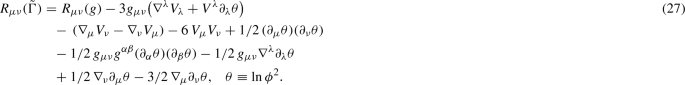
Finally, from solution (25) and (2) we compute $R_{\mu \nu }(\tilde{\Gamma })$ and scalar curvature¹⁸$R(\tilde{\Gamma },g)$

$$\begin{aligned} R(\tilde{\Gamma },g)= & {} R(g)-6 g^{\mu \nu } \nabla _\mu \nabla _\nu \ln \phi -6 (\nabla _\mu \ln \phi )^2\nonumber \\&-12 \big (\nabla _\lambda V^\lambda + V^\lambda \partial _\lambda \ln \phi ^{{2}}\big ) -6 V_\mu \, V^\mu . \end{aligned}$$

(28)

R(g) is here the usual Ricci scalar and $V_\lambda = w_\lambda -\partial _\lambda \ln \phi ^2$. Using (28) in (17), then finally

$$\begin{aligned} L_2= & {} \sqrt{g}\,\left\{ -\frac{\xi _0}{12} \left[ \phi ^2 R(g) +6 (\partial _\mu \phi )^2\right] \right. \nonumber \\&\left. +\frac{\xi _0}{2} \phi ^2 \,(v_\mu -\partial _\mu \ln \phi ^2)^2 -\frac{1}{4\, \alpha ^2} F_{\mu \nu }^2-\frac{\xi _0}{4!}\,\phi ^4\right\} . \end{aligned}$$

(29)

This is the “onshell” Lagrangian of EP quadratic gravity of Eq. (14) and is gauged scale invariant. $L_2$ is a second-order scalar–vector–tensor theory of gravity which is ghost-free according to [92] for a torsion-free connection as here (this is also obvious from (30) below). This is relevant since initial action (14) which (offshell) was of second order is actually a four-derivative theory in the metric¹⁹ for $\tilde{\Gamma }$ onshell; indeed, $R(\tilde{\Gamma },g)^2$ in (14) with replacement (28) contains the higher derivative term $R^2(g)+\cdots$; this four-derivative theory has an equivalent second-order formulation with additional $\phi$, as shown in Eq. (29). Finally, if $v_\mu =\partial _\mu \ln \phi ^2$ (“pure gauge”), the model is Weyl integrable and (29) recovers (12).

Lagrangian (29) (also initial (15)) is similar to that of Weyl quadratic gravity [26, 27], up to a Weyl tensor-squared term not included here. However, unlike in Weyl theory, here $\tilde{\Gamma }$ is $\phi$-dependent; also, in Weyl theory non-metricity follows from the underlying Weyl conformal geometry, while here it emerges after we determine $\tilde{\Gamma }$ from its equation of motion.

3.2 Stueckelberg breaking to Einstein–Proca action

Given $L_2$ in (29) with gauged scale symmetry we would like to “fix the gauge”. We choose the Einstein gauge obtained from (29) by transformations (4) and (18) of a special $\Omega ^2=\xi _0\phi ^2/(6 M^2)$ fixing $\phi$ to a constant ($\langle \phi \rangle \not =0$). After removing the hats ( $\hat{}$ ) on transformed g,$v_\mu$, R, we find

$$\begin{aligned} L_2= & {} \sqrt{g}\, \left\{ -\frac{1}{2} M^2 R(g) +3\, M^2 \,v_\mu \,v_\nu \, g^{\mu \nu } \right. \nonumber \\&\left. -\frac{1}{4 \alpha ^2} F_{\mu \nu }^2-\frac{3}{2\xi _0} M^4\right\} . \end{aligned}$$

(30)

This is the Einstein–Proca action for the gauge field $v_\mu$ with a positive cosmological constant, in which we identified M with the Planck scale (M) as seen from Eq. (29)

$$\begin{aligned} M^2\equiv \xi _0\langle \phi \rangle ^2/6. \end{aligned}$$

(31)

The initial gauged scale invariance is broken by a gravitational Stueckelberg mechanism [74,75,76]: the massless $\phi$ is not part of the action anymore, but $v_\mu$ has become massive, after “absorbing” the derivative $\partial _\mu (\ln \phi )$ of the Stueckelberg field (dilaton) in Eq. (29). Note that $\partial _\mu (\ln \phi )$ is actually the Goldstone of special conformal symmetry – this Goldstone is not independent but is determined by the derivative of the dilaton [93]. The number of degrees of freedom (dof) other than graviton is conserved in going from (29) to (30), as it should be for spontaneous breaking: massless $v_\mu$ and dynamical $\phi$ are replaced by massive $v_\mu$ (dof = 3). The mass of $v_\mu$ is $m_v^2\!=6 \alpha ^2 M^2$ which is near Planck scale M (unless one fine-tunes $\alpha \ll 1$).

Using the same transformation $\Omega$, from (24)

$$\begin{aligned} {\tilde{\nabla }}_{\lambda } g_{\mu \nu }=(-2)(g_{\mu \nu } v_\lambda -g_{\mu \lambda } v_\nu -g_{\nu \lambda } v_\mu ). \end{aligned}$$

(32)

This has a solution $\tilde{\Gamma }$ that is immediate from (25) for $\phi$ constant and $V_\lambda$ replaced by $v_\lambda$. Finally, after the massive field $v_\mu$ decouples, metricity is recovered below $m_v$, so ${\tilde{\nabla }}_{\lambda } g_{\mu \nu }=0$ and $\tilde{\Gamma }=\Gamma (g)$. Briefly, Einstein action is a “low energy” limit of Einstein–Palatini quadratic gravity, and the Planck scale $M\sim \langle \phi \rangle$ is a phase transition scale (up to coupling $\alpha$).²⁰

For comparison, in Weyl quadratic gravity e.g. [26, 27], non-metricity is different²¹

$$\begin{aligned} {\tilde{\nabla }}_\lambda g_{\mu \nu }=-g_{\mu \nu }\,v_\lambda . \end{aligned}$$

(33)

Interestingly the different non-metricity of these theories (giving different $\tilde{\Gamma }$) has phenomenological impact, see Sect. 5. In both theories the non-metricity scale is $m_v\sim \,$Planck scale and is large enough (current bounds [77, 78] are low $\sim$ TeV) to suppresses unwanted effects e.g. atomic spectral lines spacing. Past critiques of non-metricity assumed a massless $v_\mu$.

Finally, let us remark that the above spontaneous symmetry breaking mechanism for initial action (14) is special since it takes place in the absence of matter. Indeed, the necessary scalar (Stueckelberg) field $\ln \phi$ was not added ad-hoc to this purpose, as usually done in the literature; instead, this field was “extracted” from the $R^2$ term in the initial, symmetric action (14) and is thus of geometric origin. This situation is similar to Weyl quadratic gravity where this mechanism was first noticed [26, 27].

3.3 Conserved current

Equations (20) and (22) show there is now a non-trivial current due to dynamical $v_\mu \sim \tilde{\Gamma }_\mu$

$$\begin{aligned} J^\mu =\sqrt{g}\, g^{\rho \mu } \,\phi \, (\partial _\rho -1/2\, v_\rho )\,\phi ,\quad \nabla _\mu J^\mu =0, \end{aligned}$$

(34)

This is conserved since $F_{\mu \nu }$ in (20) is anti-symmetric. To obtain (34) we used that the lhs of (20) and of (22) (with $\lambda =\nu$) are equal and replaced $V_\lambda =v_\lambda -\partial _\lambda \ln \phi ^2$. The current $J^\mu$ is the same as that in Weyl quadratic gravity [26] (Eq. 18) which has similar symmetry but different non-metricity. The presence of this conserved current extends to the case of the gauged scale symmetry a similar conservation for a global scale symmetry [64]. For a Friedmann–Robertson–Walker metric with $\phi$ only t-dependent such current conservation in the global case naturally leads to $\phi$=constant [64] and a breaking of scale symmetry. In our case, since Eq. (30) has $\phi$=constant (assumed $\langle \phi \rangle \not =0$), then from (34) one has $\nabla _\mu v^\mu =0$ which is a condition similar to that for a Proca (massive) gauge field, leaving 3 degrees of freedom for $v_\mu$ in (30).

4 Palatini quadratic gravity: adding matter

In this section we re-do the previous analysis in the presence of a scalar $\chi$ which can be the SM Higgs, with non-minimal coupling with Palatini connection to the EP quadratic gravity.

The general Lagrangian of the field $\chi$, with gauged scale invariance, Eqs. (4) and (18) is

$$\begin{aligned} L_3= & {} \sqrt{g}\,\left[ \, \frac{\xi _0}{4!}\,R(\tilde{\Gamma },g)^2 - \frac{1}{4 \alpha ^2}\, F_{\mu \nu }^2 - \frac{1}{12} \,\xi _1\chi ^2\,R(\tilde{\Gamma },g)\right. \nonumber \\&\left. +\frac{1}{2} \,({\tilde{D}}_\mu \chi )^2 - \frac{\lambda _1}{4!}\chi ^4\right] , \end{aligned}$$

(35)

with the potential dictated by this symmetry and with

$$\begin{aligned} {\tilde{D}}_\mu \chi =(\partial _\mu -1/2\,v_\mu )\,\chi . \end{aligned}$$

(36)

Under (4) and (18) the Weyl-covariant derivative transforms as $\hat{{\tilde{D}}}_\mu {\hat{\chi }}=(1/\Omega )\, {\tilde{D}}_\mu \chi$. As in previous sections, replace $R(\tilde{\Gamma },g)^2\!\rightarrow \! -2 \phi ^2 R(\tilde{\Gamma },g)-\phi ^4$ to find an equivalent “linearised” $L_3$

$$\begin{aligned} L_3&=\sqrt{g}\,\left[ \, - \frac{1}{2} \,\rho ^2\,R(\tilde{\Gamma },g) - \frac{1}{4 \alpha ^2}\,F_{\mu \nu }^2 \right. \nonumber \\&\quad \left. + \frac{1}{2} \,({\tilde{D}}_\mu \chi )^2 -{{\mathcal {V}}}(\chi ,\rho ) \right] , \end{aligned}$$

(37)

where

$$\begin{aligned}&{{\mathcal {V}}}(\chi ,\rho )\equiv \frac{1}{4!}\,\left[ \frac{1}{\xi _0} (6\rho ^2-\xi _1\chi ^2)^2 + \lambda _1\chi ^4\right] ,\nonumber \\&\quad \text {and}\quad \rho ^2=\frac{1}{6}\,(\xi _1\chi ^2+\xi _0\phi ^2). \end{aligned}$$

(38)

Notice that we also replaced the scalar field $\phi$ by the new, radial direction field $\rho$; $\ln \rho$ transforms as $\ln \rho \rightarrow \ln \rho -\ln \Omega$ and acts as the (would-be) Goldstone of the symmetry.

The equation of motion for $\tilde{\Gamma }_{\mu \nu }^\lambda$ is similar to (19) but with a replacement $\phi \rightarrow \rho$ and with an additional contribution from the kinetic term of $\chi$. Following the same steps as in the previous section, we eliminate the contributions of the kinetic terms of $\chi$ and $v_\mu$ to the equation of $\tilde{\Gamma }$ and find an equation similar to (21) with $\phi \rightarrow \rho$:

$$\begin{aligned} {\tilde{\nabla }}_\lambda (\sqrt{g}g^{\mu \nu }\rho ^2) -\frac{1}{5} \Big \{ \delta _\lambda ^\nu \, {\tilde{\nabla }}_\sigma (\sqrt{g}g^{\sigma \mu }\rho ^2)+(\mu \leftrightarrow \nu ) \Big \}=0.\nonumber \\ \end{aligned}$$

(39)

This gives (see previous section):

$$\begin{aligned} {\tilde{\nabla }}_\lambda (\rho ^2 g_{\mu \nu }) =(-2)\rho ^2 (g_{\mu \nu }\,V_\lambda -g_{\mu \lambda } V_\nu - g_{\nu \lambda } V_\mu ), \end{aligned}$$

(40)

where $V_\mu =(-1/2){\tilde{\nabla }}_\mu \ln (\sqrt{g}\rho ^4)=v_\mu -\partial _\mu \ln \rho ^2$. From (40) one finds the solution for Palatini connection $\tilde{\Gamma }_{\mu \nu }^\alpha$ in terms of $v_\mu \sim \tilde{\Gamma }_\mu$, with a result similar to (25) but with $\phi \rightarrow \rho$. We use this solution for the connection back in the action and find for $\tilde{\Gamma }$ onshell²²

$$\begin{aligned} L_3= & {} \sqrt{g}\left\{ \frac{-1}{2} [\rho ^2 R(g) + 6 (\partial _\mu \rho )^2] + 3 \rho ^2 (v_\mu -\partial _\mu \ln \rho ^2)^2 \right. \nonumber \\&\left. -\frac{1}{4 \alpha ^2} \,F_{\mu \nu }^2 +\frac{1}{2} ({\tilde{D}}_\mu \chi )^2 - {{\mathcal {V}}}(\chi ,\rho )\right\} . \end{aligned}$$

(41)

$L_3$ has a gauged scale symmetry and extents (29) in the presence of scalar field $\chi$.

Finally, we choose the Einstein gauge by using transformation (4) and (18) of a particular $\Omega \!=\!\rho /M$ which essentially sets ${\hat{\rho }}$ to a constant (vev). In terms of the new variables (with a hat) we find

$$\begin{aligned} L_3= & {} \sqrt{{\hat{g}}}\, \left\{ -\frac{1}{2} M^2\,R({\hat{g}}) +3 M^2 {\hat{v}}_\mu {\hat{v}}^\mu -\frac{1}{4 \alpha ^2} {\hat{F}}_{\mu \nu }^2\right. \nonumber \\&\left. +\frac{1}{2}(\hat{{\tilde{D}}}_\mu {\hat{\chi }})^2 -{{\mathcal {V}}}({\hat{\chi }},M) \Big ]\right\} , \end{aligned}$$

(42)

with ${\hat{{\tilde{D}}}}_\mu {\hat{\chi }}=(\partial _\mu -1/2\,\,{\hat{v}}_\mu ){\hat{\chi }}$ and we identify M with the Planck scale ($M=\langle {\hat{\rho \rangle }}$). As in the absence of matter, we obtained the Einstein–Proca action of a gauge field that became massive after Stueckelberg mechanism of “absorbing” the derivative term $\partial _\mu (\ln \rho )$. A canonical kinetic term of ${\hat{\chi }}$ remained present in the action, since only one degree of freedom (radial direction $\rho$) was “eaten” by $v_\mu$. The mass of $v_\mu$ is $m_v^2=6 \alpha ^2 M^2$. The potential becomes

$$\begin{aligned} {{\mathcal {V}}}= \frac{3 M^4}{2\,\xi _0} \left[ 1-\frac{\xi _1{\hat{\chi }}^2}{6 \,M^2} \right] ^2 + \frac{\lambda _1}{4!}\,{\hat{\chi }}^4. \end{aligned}$$

(43)

For a “standard” kinetic term for ${\hat{\chi }}$, similar to a “unitary gauge” in electroweak case, we remove the coupling ${\hat{v}}^\mu \partial _\mu {\hat{\chi }}$ in the Weyl-covariant derivative in (42) by a field redefinition

$$\begin{aligned} {{\hat{v}}_\mu ^\prime }= & {} {\hat{v}}_\mu - \partial _\mu \ln \cosh ^2 \left[ \frac{\sigma }{2 M\sqrt{6}}\right] ,\nonumber \\ {\hat{\chi }}= & {} 2 M\sqrt{6}\,\sinh \left[ \frac{\sigma }{2 M\sqrt{6}}\right] , \end{aligned}$$

(44)

which replaces ${\hat{\chi \rightarrow \sigma }}$. After some algebra, we find the final Lagrangian

$$\begin{aligned} L_3= & {} \sqrt{{\hat{g}}}\, \left\{ -\frac{1}{2} M^2\,\hat{R} + 3 M^2 \cosh ^2 \left[ \frac{\sigma }{2 M\sqrt{6}}\right] {\hat{v}}^\prime _\mu {\hat{v}}^{\prime \,\mu } \right. \nonumber \\&\left. -\frac{1}{4 \alpha ^2} {\hat{F}}^{\prime \, 2}_{\mu \nu } +\frac{{\hat{g}}^{\mu \nu }}{2}\partial _\mu \sigma \partial _\nu \sigma -{{\hat{{{\mathcal {V}}}}}}(\sigma )\right\} \end{aligned}$$

(45)

with

$$\begin{aligned} {{\hat{{{\mathcal {V}}}}}(\sigma )}= & {} {\hat{{{\mathcal {V}}}}}_0\, \left\{ \left[ 1-4 \xi _1\sinh ^2 \frac{\sigma }{2 M\sqrt{6}}\right] ^2 \right. \nonumber \\&\left. + 16 \,\lambda _1 \xi _0 \sinh ^4\frac{\sigma }{2 M\sqrt{6}} \,\right\} ,\quad {\hat{{{\mathcal {V}}}}}_0\equiv \frac{3}{2} \frac{M^4}{\xi _0}. \end{aligned}$$

(46)

In (45) one finally rescales ${\hat{v}}^\prime _\mu \rightarrow \alpha \,{\hat{v}}_\mu ^\prime$ for a canonical gauge kinetic term.

For small field values, $\sigma \ll M$, then ${\hat{\chi }}\approx \sigma$ (up to ${{\mathcal {O}}}(\sigma ^3/M^2)$) and a SM Higgs-like potential is recovered,²³ see Eq. (43). For $\xi _1>0$ it has spontaneous breaking of the symmetry carried by $\sigma$ i.e. electroweak (EW) symmetry if $\sigma$ is the Higgs; this is triggered by the non-minimal coupling to gravity ($\xi _1\not = 0$) and Stueckelberg mechanism. The negative mass term originates in (38) due to the $\phi ^4$ term (itself induced by ${\tilde{R}}^2$). The mass $m_\sigma ^2\propto \xi _1 M^2/\xi _0$ may be small enough, near the EW scale by tuning $\xi _1\ll \xi _0$. It may be interesting to study if the gauged scale symmetry brings some “protection” to $m_\sigma$ at the quantum level.

$L_3$ of (45) is similar to that in Weyl quadratic gravity with a non-minimally coupled scalar/Higgs field [26,27,28],²⁴ up to a rescaling of the couplings ($\xi _1$, $\lambda _1$) and fields ($\sigma$). This difference is due to the different non-metricity of the two theories, Eqs. (32) and (33). Both cases provide a gauged scale invariant theory of quadratic gravity coupled to matter. They both recover Einstein gravity in their broken phase, see Eq. (45), and also metricity below the scale $m_v\sim \alpha M$ ($\alpha \le 1$). This result may be more general – it may apply to other theories with this symmetry and can be used for model building.

To conclude, mass generation (Planck scale, $v_\mu$ mass) and Einstein gravity emerge naturally from spontaneous breaking of gauged scale symmetry in Einstein–Palatini theories, even in the absence of matter. Actions (14) and (35) were inspired by Weyl quadratic gravity of similar breaking [27]; but in a more general case, additional operators may be present in (14) and (35); for a list of all quadratic operators and a complementary study see [14]. The mechanism of symmetry breaking should remain valid in their presence if one includes the terms in (14): $R^2$ that ’supplied’ the scalar field and $R_{[\mu \nu ]}^2$ generating the symmetry and non-metricity. However, in such general case it is unclear that one can still solve algebraically the second-order differential equations of motion of $\tilde{\Gamma }$ (Eq. (19)) without simplifying assumptions, since these equations acquire new terms of different indices structure and new states will be present (ghosts, etc.).

5 Palatini $R^2$ inflation

In this section we consider an application to inflation of the action in the previous section.

For large field values, the potential in (46) can also be used for inflation (hereafter Palatini $R^2$ inflation), with $\sigma$ as the inflaton.²⁵ For a Friedmann–Robertson–Walker metric (FRW) $(1,-a^2(t),-a^2(t), -a^2(t))$ and compatible background $v_\mu (t)=(v_0(t),0,0,0)$ the gauge fixing condition $\nabla _\mu v^\mu =0$ gives that $v_\mu (t)$ redshifts to zero $v_\mu (t)\sim 1/a^3(t)$. Then the coupling $v_\mu -\sigma$ in (45) is vanishing and therefore $v_\mu (t)$ cannot affect inflation; this means we have single-field inflation of potential (46) and standard slow-roll formulae can be used. Further, since M is just a phase transition scale, field values $\sigma \ge M$ are natural. ${\hat{{{\mathcal {V}}}}}(\sigma )$ is similar to that in Weyl gravity $R^2$-inflation, see [28, 47] for a detailed analysis²⁶; however, as mentioned, the couplings and field normalization in the potential differ (for same initial couplings and non-metricity trace); hence the spectral index $n_s$ and tensor-to-scalar ratio r are different, too, and need to be analyzed separately.

The potential is shown in Fig. 1 for perturbative values of the couplings relevant for successful inflation. This demands $\lambda _1 \xi _0\ll \xi _1^2\ll 1$, with the first relation from demanding that the initial energy be larger than at the end of inflation ${\hat{{{\mathcal {V}}}}}_0>{\hat{{{\mathcal {V}}}}}_{\mathrm{min}}$, respected by choosing a small enough $\lambda _1$ for given $\xi _{0,1}$. Therefore, we shall work in the leading order in $(\lambda _1\xi _0)$.

The slow-roll parameters are:

$$\begin{aligned} \epsilon= & {} \frac{M^2}{2} \left\{ \frac{{\hat{{{\mathcal {V}}}^\prime }}(\sigma )}{{\hat{{{\mathcal {V}}}}}(\sigma )}\right\} ^2 = \frac{{4}}{3}\, \,\xi _1^2\, \sinh ^2 \frac{\sigma }{M\sqrt{6}} +{{\mathcal {O}}}(\xi _1^3)\, \end{aligned}$$

(47)

$$\begin{aligned} \eta= & {} M^2\,\frac{{\hat{{{\mathcal {V}}}}}^{\prime \prime }(\sigma )}{{\hat{{{\mathcal {V}}}}}(\sigma )}= -\frac{2}{3}\,\xi _1 \,\cosh {\frac{\sigma }{M\sqrt{6}}}+{{\mathcal {O}}}(\xi _1^2). \end{aligned}$$

(48)

Then

$$\begin{aligned} n_s = 1 + 2\,\eta _* - 6\, \epsilon _*= 1 -\frac{4}{3}\,\xi _1 \,\cosh \frac{\sigma _*}{M\sqrt{6}}+{{\mathcal {O}}}(\xi _1^2),\nonumber \\ \end{aligned}$$

(49)

where $\sigma _*$ is the value of $\sigma$ at the horizon exit. With $r=16 \epsilon _*$ we have²⁷

$$\begin{aligned} r={12}\, (1- n_s)^2+{{\mathcal {O}}}(\xi _1^2). \end{aligned}$$

(50)

The contribution of $\epsilon$ is subleading for small $\xi _1$ considered here. The slope of the curves in the plane $(n_s,r)$, shown in leading order in (50), is steeper than in Weyl $R^2$ inflation [28] (or Starobinsky model) where $r=3 (1-n_s)^2+{{\mathcal {O}}}(\xi _1^2)$.

Fig. 1

Left plot: The potential ${\hat{{{\mathcal {V}}}}}(\sigma )/{\hat{{{\mathcal {V}}}}}_0$ for $\lambda _1\xi _0=10^{-10}\!\ll \! \xi _1^2$ with different $\xi _1\!\ll \! 1$. For larger $\lambda _1\xi _0$ the curves move to the left while the minimum of the rightmost ones is lifted. Larger values of $\lambda _1\xi _0$ are allowed, but inflation becomes less likely when $\lambda _1\xi _0\sim \xi _1^2$. The flat region is wide for a large range of $\sigma$, with the width controlled by $1/\sqrt{\xi }_1$ while its height is ${\hat{{{\mathcal {V}}}}}_0\propto 1/\xi _0$. We have ${\hat{{{\mathcal {V}}}}}/{\hat{{{\mathcal {V}}}}}_{\mathrm{min}}\propto \xi _1^2/(\lambda _1\xi _0)$. Right plot: The values of $(n_s,r)$ for different values of $\xi _1$ that enable values of $n_s=0.9670\pm 0.0037$ at 68% CL (blue band) and 95% CL (light blue region). For each curve $N=60$ efolds is marked by a red point and the dark blue interval corresponds to $55\le N\le 65$. Curves of $\xi _1<10^{-3}$ are degenerate with the red one while those with $\xi _1>2.5 \times 10^{-2}$ have $N>65$

The exact numerical results for $(n_s,r)$ in our model, for different e-folds number N, are shown in Fig. 1. From experimental data $n_s=0.9670\pm 0.0037$ ($68\%$ CL) and $r<0.07$ ($95\%$ CL) from Planck 2018 (TT, TE, EE + low E + lensing + BK14 + BAO) [105]. Using this data, Fig. 1 (right plot) shows that a specific, small range for r is predicted in our model for the current range for $n_s$ at $95\%$ CL:

$$\begin{aligned} N=60,\quad 0.007 \le r\le 0.010,\quad [\text {Palatini }R^2\text { inflation}]. \end{aligned}$$

(51)

Similar values for r can be read from Fig. 1 for $55\le N\le 65$. The lower bound on r comes from that for $n_s$ while the upper one corresponds to a saturation limit, $\xi _1\rightarrow 0$, with values $\xi _1<10^{-3}$ having similar $(n_s,r)$. One should also respect the constraint $\lambda _1\le \xi _1^2/\xi _0$, giving $\lambda _1\sim 10^{-12}$ or smaller (with the CMB anisotropy constraint $\xi _0\ge 6.89\times 10^8$).

For comparison, in Weyl $R^2$-inflation for same $n_s$ at $95\%$ CL one has a smaller r [28, 47]

$$\begin{aligned} N=60, \quad 0.00257\le r\le 0.00303,\quad [\text {Weyl }R^2 \text { inflation}].\nonumber \\ \end{aligned}$$

(52)

The different range for r in Eq. (51) versus Eq. (52) is important since it enables us to distinguish these two inflation models based on gauged scale invariance, and is due to their different non-metricity.²⁸$^,$²⁹ Such values for $r\sim 10^{-3}$ will soon be reached by various CMB experiments [79,80,81] that will then be able test both models. This establishes an interesting connection between non-metricity and testable inflation predictions.

Similar values for r were found in other recent inflation models in Palatini $R^2$ gravity [102,103,104] but these are not gauged scale invariant. In the absence of this symmetry, other successful models (e.g. Starobinsky model [106]) have corrections to r from higher curvature operators ($R^4$, etc.) of unknown coefficients [108]. Such operators (and their corrections) are not allowed here because they must be suppressed by some effective scale whose presence would violate scale invariance.³⁰ Another advantage is that due to the gauged scale symmetry Palatini $R^2$ inflation is allowed by black-hole physics (similarly for Weyl $R^2$ inflation [28]), in contrast to models of inflation with global scale symmetry.³¹

6 Conclusions

At a fundamental level gravity may be regarded as a theory of connections. An example is the Einstein–Palatini (EP) approach to gravity where the connection ($\tilde{\Gamma }$) is apriori independent of the metric, and is determined by its equation of motion, from the action. For simple actions $\tilde{\Gamma }$ plays an auxiliary role (no dynamics) and can be solved algebraically. In particular, for Einstein action in the EP approach one finds that the connection is actually equal to the Levi-Civita connection (of the metric formulation); then Einstein gravity is recovered, so the metric and EP approaches are equivalent. However, this equivalence is not true in general, for complicated actions, etc. In this work we considered quadratic gravity actions in the EP approach, with the goal to show that, while this equivalence does not hold true, one can still find actions that recover dynamically the Levi-Civita connection, metricity, Einstein gravity and Planck mass in some “low-energy” limit, even in the absence of matter.

We studied EP quadratic gravity given by $R(\tilde{\Gamma },g)^2+R_{[\mu \nu ]}(\tilde{\Gamma })^2$ which has local scale symmetry. $R_{[\mu \nu ]}(\tilde{\Gamma })^2$ can be regarded as a gauge kinetic term for the vector field $v_\mu \sim \tilde{\Gamma }_\mu -\Gamma _\mu$ where $\tilde{\Gamma }_\mu$ ($\Gamma _\mu$) denotes the trace of the Palatini (Levi-Civita) connections, respectively. Hence this theory actually has a gauged scale symmetry, with $v_\mu$ the Weyl gauge field. A consequence of this symmetry is that the theory is non-metric i.e. ${\tilde{\nabla }}_\mu g_{\alpha \beta }\not =0$ (due to dynamical $v_\mu \sim \tilde{\Gamma }_\mu$). At the same time, the equations of motion of the connection ($\tilde{\Gamma }$) become complicated second-order differential equations and we showed how to solve them algebraically in terms of an auxiliary scalar $\phi$ that “linearises” the $R(\tilde{\Gamma },g)^2$ term. While initially the action appears to be of second order, for $\tilde{\Gamma }$ onshell it is a higher derivative theory since $R(\tilde{\Gamma },g)^2$ contains a (four-derivative) metric contribution $R(g)^2+\cdots$. We showed that for $\tilde{\Gamma }$ onshell, the action is equivalent to a second-order theory in which the initial auxiliary field $\phi$ has become dynamical, while preserving the symmetry of the theory.

The main result is that our EP quadratic gravity action has an elegant spontaneous breaking mechanism of gauged scale invariance and mass generation valid even in the absence of matter; in this, the necessary scalar field ($\phi$) was not added ad-hoc to this purpose (as usually done), but was “extracted” from the $R^2$ term, as mentioned, being of geometric origin. The derivative $\partial _\mu \ln \phi$ of this field acting as a Stueckelberg field is “eaten” by $v_\mu$ which becomes massive, of mass $m_v$ proportional to the Planck scale $M\sim \langle \phi \rangle$. One obtains the Einstein–Proca action for the gauge field $v_\mu$ and a positive cosmological constant. This is a “low-energy” broken phase of the initial action. Below the scale $m_v\sim M$, the Proca field $v_\mu$ decouples and metricity and the Einstein action are recovered. Non-metricity effects are strongly suppressed by a large scale ($\propto M$), which is important for the theory to be viable.

The above results remain valid in the presence of scalar matter (Higgs, etc.) with a (perturbative) non-minimal coupling to this theory with a Palatini connection; in such case and following the Stueckelberg mechanism, the scalar potential also has a breaking of the symmetry under which this scalar is charged, e.g. electroweak symmetry in the Higgs case. This is relevant for building models with this symmetry for physics beyond the SM.

To summarise, Einstein–Palatini quadratic gravity $R(\tilde{\Gamma },g)^2+R_{[\mu \nu ]}^2(\tilde{\Gamma })$ is a gauged theory of scale invariance that is spontaneously broken to the Einstein–Proca action for the Weyl field with a positive cosmological constant; if initial action also contains (non-minimally coupled) scalar fields with Palatini connection, a scalar potential is also present.

This picture is similar to a recent analysis for the original Weyl quadratic gravity, despite the different non-metricity of these two theories. With hindsight, this is not too surprising, since in both theories there is a gauged scale symmetry and the connection is not fixed by the metric, except that in Weyl gravity non-metricity is present from the onset (due to underlying Weyl conformal geometry) while here it emerges for $\tilde{\Gamma }$ onshell. It is worth studying further the relation of these two theories, by including any remaining operators (on the Einstein–Palatini side) that can have this symmetry.

There are also interesting predictions from inflation. While the scalar potential is Higgs-like for small field values ($\ll M$), for large field values it can be used for inflation. With the Planck scale M a simple phase transition scale, field values above M are natural. The inflaton potential is similar to that in Weyl quadratic gravity, up to couplings and field redefinitions (due to different non-metricity of the two theories). We find a specific prediction for the tensor-to-scalar ratio, $0.007\le r \le 0.01$, for the current value of the spectral index at $95\%$ CL. This value of r is mildly larger than that predicted by inflation in Weyl gravity. This enables us to distinguish and test these two theories by future CMB experiments that will reach such values of r. It also establishes an interesting connection between non-metricity and inflation predictions.

Appendix

For a self-contained presentation, we include here basic aspects of the Palatini formalism used in the text. In the (pseudo-)Riemannian geometry, the Levi-Civita connection $\Gamma (g)$ is determined by the metric. In general, however, the connection can be introduced without reference to $g_{\mu \nu }$. In the Palatini approach the connection $\tilde{\Gamma }$ is apriori independent of the metric and is determined by the equations of motion. To ensure the covariant derivatives transform under coordinate change ($x\rightarrow x'(x)$) as true tensors, Palatini connection has a transformation law

$$\begin{aligned} \tilde{\Gamma }^{ ' \lambda }_{\mu \nu }= \frac{\partial x^{\alpha }}{\partial x^{' \mu }} \frac{\partial x^{\beta }}{\partial x^{' \nu }}\,\, \frac{\partial x^{' \lambda }}{\partial x^{\rho }}\, \tilde{\Gamma }^{\rho }_{\alpha \beta } + \frac{\partial x^{' \lambda }}{\partial x^\sigma } \frac{\partial ^2 x^\sigma }{\partial x^{' \mu } \partial x^{' \nu }} \end{aligned}$$

(53)

with $\tilde{\Gamma }'=\tilde{\Gamma }'(x')$, $\tilde{\Gamma }=\tilde{\Gamma }(x)$. In the text we also assumed $\tilde{\Gamma }_{\mu \nu }^\rho =\tilde{\Gamma }_{\nu \mu }^\rho$ (no torsion). The Levi-Civita connection $\Gamma _{\mu \nu }^\lambda (g)$ has a similar transformation

$$\begin{aligned} \Gamma ^{ ' \lambda }_{\mu \nu }(g)= \frac{\partial x^{\alpha }}{\partial x^{' \mu }} \frac{\partial x^{\beta }}{\partial x^{' \nu }}\,\, \frac{\partial x^{' \lambda }}{\partial x^{\rho }}\, \Gamma ^{\rho }_{\alpha \beta }(g) + \frac{\partial x^{' \lambda }}{\partial x^\sigma } \frac{\partial ^2 x^\sigma }{\partial x^{' \mu } \partial x^{' \nu }}. \end{aligned}$$

(54)

Note that the difference of these connections transforms as a tensor

$$\begin{aligned} \tilde{\Gamma }^{ ' \lambda }_{\mu \nu }-\Gamma ^{ ' \lambda }_{\mu \nu }(g)= \frac{\partial x^{\alpha }}{\partial x^{' \mu }} \frac{\partial x^{\beta }}{\partial x^{' \nu }}\,\, \frac{\partial x^{' \lambda }}{\partial x^{\rho }}\, (\tilde{\Gamma }^{\rho }_{\alpha \beta }(x) -\Gamma ^{\rho }_{\alpha \beta }(g)). \end{aligned}$$

(55)

Setting $\lambda =\nu$ and with the notation $\tilde{\Gamma }_\mu \equiv \tilde{\Gamma }_{\mu \nu }^\nu$, $\Gamma _\mu \equiv \Gamma _{\mu \nu }^\nu$, etc., then

$$\begin{aligned} \tilde{\Gamma }_\mu ' - \Gamma _\mu ' (g)= \frac{\partial x^{\alpha }}{\partial x^{' \mu }}\, (\tilde{\Gamma }_\alpha -\Gamma _\alpha (g)) \end{aligned}$$

(56)

and therefore $v_\mu$ introduced in Sect. 3 transforms as a covariant vector

$$\begin{aligned} v_\mu '(x')= \frac{\partial x^{\alpha }}{\partial x^{' \mu }} v_\alpha (x) \end{aligned}$$

(57)

Further, the covariant derivatives used in the text are

$$\begin{aligned} {\tilde{\nabla }}_\nu v_\mu =\partial _\nu v_\mu -\tilde{\Gamma }^\lambda _{\mu \nu } v_\lambda , \qquad {\tilde{\nabla }}_\nu v^\mu =\partial _\nu v^\mu +\tilde{\Gamma }^\mu _{\lambda \nu } v^\lambda . \end{aligned}$$

(58)

One also has $\tilde{\nabla }_\lambda g_{\mu \nu }=\partial _\lambda g_{\mu \nu } -\tilde{\Gamma }^\rho _{\mu \lambda } g_{\rho \nu } -\tilde{\Gamma }^\rho _{\nu \lambda } g_{\rho \mu }$, also used in the text.

In Sect. 3 we introduced the gauge field $v_\mu$ in Eq. (16). This is general. For example, in Weyl gravity of similar gauged scale symmetry, an identical formula exists for the gauge field. To see this, note that in Weyl gravity [26, 27], see also Eq. (33) in the text, non-metricity is different from EP quadratic gravity: ${\tilde{\nabla }}_\lambda g_{\mu \nu }=-v_\lambda \, g_{\mu \nu }$. Contracting this equation with $g^{\mu \nu }$ and using ${\tilde{\nabla }}_\lambda \sqrt{g}=(1/2) \sqrt{g} \,g^{\mu \nu } \, {\tilde{\nabla }}_\lambda g_{\mu \nu }$ we find $v_\lambda =(-1/2) {\tilde{\nabla }}_\lambda \ln \sqrt{g}$. This is similar to Palatini case, Eq. (26) in the text, although the connection is different. From these last two equations, by writing the action of ${\tilde{\nabla }}_\lambda$ on $g_{\mu \nu }$ one immediately finds

$$\begin{aligned} v_\mu = (1/2) (\tilde{\Gamma }_\mu -\Gamma _\mu (g)) \end{aligned}$$

(59)

with the trace of Levi-Civita connection $\Gamma _\mu (g)=\partial _\mu \ln \sqrt{g}$. Equation (59) was used as a definition for the gauge field in Einstein–Palatini quadratic gravity, Eq. (16).

References

A. Einstein, Einheitliche Feldtheories von Gravitation und Electrizitat (Sitzungber Preuss Akad. Wiss, Berlin, 1925), pp. 414–419
M. Ferraris, M. Francaviglia, C. Reina, Variational formulation of general relativity from 1915 to 1925, “Palatini’s method” discovered by Einstein in 1925. Gen. Relativ. Gravit. 14, 243–254 (1982)
For a review and references, see G.J. Olmo, Palatini approach to modified gravity: f(R) theories and beyond. Int. J. Mod. Phys. D 20, 413 (2011). arXiv:1101.3864 [gr-qc]
Another review is: T.P. Sotiriou, S. Liberati, Metric-affine f(R) theories of gravity. Ann. Phys. 322, 935 (2007). arXiv:gr-qc/0604006
T.P. Sotiriou, V. Faraoni, f(R) theories of gravity. Rev. Mod. Phys. 82, 451 (2010). arXiv:0805.1726 [gr-qc]
H.A. Buchdahl, Representation of the Einstein–Proca field by an A(4)*. J. Phys. A 12, 1235 (1979)
H.A. Buchdahl, Non-linear Lagrangians and cosmological theory. Mon. Not. R. Astron. Soc. 150, 1 (1970)
D.N. Vollick, Einstein–Maxwell and Einstein–Proca theory from a modified gravitational action. arXiv:gr-qc/0601016
D.N. Vollick, Born–Infeld–Einstein theory with matter. Phys. Rev. D 72, 084026 (2005). arXiv:gr-qc/0506091
S. Cotsakis, J. Miritzis, L. Querella, Variational and conformal structure of nonlinear metric connection gravitational Lagrangians. J. Math. Phys. 40, 3063 (1999). arXiv:gr-qc/9712025
B. Shahid-Saless, First order formalism treatment of R + R**2 gravity. Phys. Rev. D 35, 467 (1987)
E.E. Flanagan, Palatini form of 1/R gravity. Phys. Rev. Lett. 92, 071101 (2004). arXiv:astro-ph/0308111
E.E. Flanagan, Higher order gravity theories and scalar tensor theories. Class. Quantum Gravity 21, 417 (2003). arXiv:gr-qc/0309015
M. Borunda, B. Janssen, M. Bastero-Gil, Palatini versus metric formulation in higher curvature gravity. JCAP 0811, 008 (2008). arXiv:0804.4440 [hep-th]
L. Järv, M. Rünkla, M. Saal, O. Vilson, Nonmetricity formulation of general relativity and its scalar–tensor extension. Phys. Rev. D 97(12), 124025 (2018). arXiv:1802.00492 [gr-qc]
R. Percacci, E. Sezgin, New class of ghost- and tachyon-free metric affine gravities. Phys. Rev. D 101(8), 084040 (2020). arXiv:1912.01023 [hep-th]
L. Querella, Variational principles and cosmological models in higher order gravity. arXiv:gr-qc/9902044
V. Vitagliano, T.P. Sotiriou, S. Liberati, The dynamics of generalized Palatini theories of gravity. Phys. Rev. D 82, 084007 (2010). arXiv:1007.3937 [gr-qc]
G. Allemandi, A. Borowiec, M. Francaviglia, S.D. Odintsov, Dark energy dominance and cosmic acceleration in first order formalism. Phys. Rev. D 72, 063505 (2005). arXiv:gr-qc/0504057 [gr-qc]
A. Kozak, A. Borowiec, Palatini frames in scalar–tensor theories of gravity. Eur. Phys. J. C 79(4), 335 (2019). arXiv:1808.05598 [hep-th]
J. Annala, Higgs inflation and higher-order gravity in Palatini formulation. PhD thesis, University of Helsinki. https://inspirehep.net/literature/1799417. Accessed April 2020
H. Weyl, Gravitation und elektrizität, Sitzungsberichte der Königlich Preussischen Akademie der Wissenschaften zu Berlin (1918), p. 465; Einstein’s critical comment appended (on atomic spectral lines changes)
H. Weyl, Eine neue Erweiterung der Relativitätstheorie (A new extension of the theory of relativity). Ann. Phys. (Leipzig) 4(59), 101–133 (1919)
H. Weyl, “Raum, Zeit, Materie”, vierte erweiterte Auflage (Julius Springer, Berlin, 1921) [Space-time-matter. Translated from German by Henry L. Brose, 1922, Methuen & Co Ltd, London]
For review and references on Weyl’s theory, see E. Scholz, The unexpected resurgence of Weyl geometry in late 20-th century physics. Einstein Stud. 14, 261 (2018). arXiv:1703.03187 [math.HO]
D.M. Ghilencea, Spontaneous breaking of Weyl quadratic gravity to Einstein action and Higgs potential. JHEP 1903, 049 (2019). arXiv:1812.08613 [hep-th]
D.M. Ghilencea, Stueckelberg breaking of Weyl conformal geometry and applications to gravity. Phys. Rev. D 101(4), 045010 (2020). arXiv:1904.06596 [hep-th]
D.M. Ghilencea, Weyl \(\text{ R}^{2}\) inflation with an emergent Planck scale. JHEP 1910, 209 (2019). arXiv:1906.11572 [gr-qc]
P.A.M. Dirac, Long range forces and broken symmetries. Proc. R. Soc. Lond. A 333, 403 (1973). https://doi.org/10.1098/rspa.1973.0070
L. Smolin, Towards a theory of space-time structure at very short distances. Nucl. Phys. B 160, 253 (1979)
H. Cheng, The possible existence of Weyl’s vector meson. Phys. Rev. Lett. 61, 2182 (1988)
I. Quiros, Scale invariant theory of gravity and the standard model of particles. E-print. arXiv:1401.2643 [gr-qc]
T. Fulton, F. Rohrlich, L. Witten, Conformal invariance in physics. Rev. Mod. Phys. 34, 442 (1962)
J.T. Wheeler, Weyl geometry. Gen. Relativ. Gravit. 50(7), 80 (2018). arXiv:1801.03178 [gr-qc]
M. de Cesare, J.W. Moffat, M. Sakellariadou, Local conformal symmetry in non-Riemannian geometry and the origin of physical scales. Eur. Phys. J. C 77(9), 605 (2017). arXiv:1612.08066 [hep-th]
H.C. Ohanian, Weyl gauge-vector and complex dilaton scalar for conformal symmetry and its breaking. Gen. Relativ. Gravit. 48(3), 25 (2016). arXiv:1502.00020 [gr-qc]
D.M. Ghilencea, H.M. Lee, Weyl symmetry and its spontaneous breaking in Standard Model and inflation. Phys. Rev. D 99, 115007 (2019) arXiv:1809.09174 [hep-th]
A. Barnaveli, S. Lucat, T. Prokopec, Inflation as a spontaneous symmetry breaking of Weyl symmetry. JCAP 01, 022 (2019) arXiv:1809.10586 [gr-qc]
J.W. Moffat, Scalar–tensor–vector gravity theory. JCAP 0603, 004 (2006). arXiv:gr-qc/0506021
L. Heisenberg, Scalar–vector–tensor gravity theories. arXiv:1801.01523 [gr-qc]
J. Beltran Jimenez, L. Heisenberg, T.S. Koivisto, Cosmology for quadratic gravity in generalized Weyl geometry. JCAP 1604(04), 046 (2016). arXiv:1602.07287 [hep-th]
J. Beltran Jimenez, T.S. Koivisto, Spacetimes with vector distortion: inflation from generalised Weyl geometry. Phys. Lett. B 756, 400 (2016). arXiv:1509.02476 [gr-qc]
C.T. Hill, Inertial symmetry breaking. arXiv:1803.06994 [hep-th]
E. Scholz, Higgs and gravitational scalar fields together induce Weyl gauge. Gen. Rel. Grav. 47(2), 7 (2015). arXiv:1407.6811 [gr-qc]
W. Drechsler, H. Tann, Broken Weyl invariance and the origin of mass. Found. Phys. 29, 1023 (1999). arXiv:gr-qc/9802044
S. Dengiz, A note on noncompact and nonmetricit quadratic curvature gravity theories. Turk. J. Phys. 42(1), 70 (2018). arXiv:1404.2714 [hep-th]
P.G. Ferreira, C.T. Hill, J. Noller, G.G. Ross, Scale-independent \(R^2\) inflation. Phys. Rev. D 100(12), 123516 (2019). arXiv:1906.03415 [gr-qc]
G. ’t Hooft, Local conformal symmetry: the missing symmetry component for space and time. Int. J. Mod. Phys. D 24(12), 1543001 (2015)
I. Bars, P. Steinhardt, N. Turok, Local conformal symmetry in physics and cosmology. Phys. Rev. D 89(4), 043515 (2014). arXiv:1307.1848 [hep-th]
G. ’t Hooft, Imagining the future, or how the Standard Model may survive the attacks. Int. J. Mod. Phys. 31(16), 1630022 (2016)
G. ’t Hooft, Local conformal symmetry in black holes, standard model, and quantum gravity. Int. J. Mod. Phys. D 26(03), 1730006 (2016)
M. Shaposhnikov, D. Zenhausern, Quantum scale invariance, cosmological constant and hierarchy problem. Phys. Lett. B 671, 162 (2009). arXiv:0809.3406 [hep-th]
R. Armillis, A. Monin, M. Shaposhnikov, Spontaneously broken conformal symmetry: dealing with the trace anomaly. JHEP 1310, 030 (2013). arXiv:1302.5619 [hep-th]
F. Bezrukov, G.K. Karananas, J. Rubio, M. Shaposhnikov, Higgs-dilaton cosmology: an effective field theory approach. Phys. Rev. D 87(9), 096001 (2013). arXiv:1212.4148 [hep-ph]
F. Gretsch, A. Monin, Perturbative conformal symmetry and dilaton. Phys. Rev. D 92(4), 045036 (2015). arXiv:1308.3863 [hep-th]
D.M. Ghilencea, Quantum implications of a scale invariant regularization. Phys. Rev. D 97(7), 075015 (2018). arXiv:1712.06024 [hep-th]
D.M. Ghilencea, Manifestly scale-invariant regularization and quantum effective operators. Phys. Rev. D 93(10), 105006 (2016). arXiv:1508.00595 [hep-ph]
D.M. Ghilencea, One-loop potential with scale invariance and effective operators. PoS CORFU 2015, 040 (2016). arXiv:1605.05632 [hep-ph]
D.M. Ghilencea, Z. Lalak, P. Olszewski, Two-loop scale-invariant scalar potential and quantum effective operators. Eur. Phys. J. C 76(12), 656 (2016). arXiv:1608.05336 [hep-th]
D.M. Ghilencea, Z. Lalak, P. Olszewski, Standard Model with spontaneously broken quantum scale invariance. Phys. Rev. D 96(5), 055034 (2017). arXiv:1612.09120 [hep-ph]
J. Kubo, M. Lindner, K. Schmitz, M. Yamada, Planck mass and inflation as consequences of dynamically broken scale invariance. Phys. Rev. D 100(1), 015037 (2019). arXiv:1811.05950 [hep-ph]
R. Foot, A. Kobakhidze, K.L. McDonald, R.R. Volkas, Poincaré protection for a natural electroweak scale. Phys. Rev. D 89(11), 115018 (2014). arXiv:1310.0223 [hep-ph]
P.G. Ferreira, C.T. Hill, G.G. Ross, Scale-independent inflation and hierarchy generation. Phys. Lett. B 763, 174 (2016). arXiv:1603.05983 [hep-th]
P.G. Ferreira, C.T. Hill, G.G. Ross, Inertial spontaneous symmetry breaking and quantum scale invariance. Phys. Rev. D 98, 116012 (2018) arXiv:1801.07676 [hep-th]
P.G. Ferreira, C.T. Hill, G.G. Ross, Weyl current, scale-invariant inflation and planck scale generation. Phys. Rev. D 95(4), 043507 (2017). arXiv:1610.09243 [hep-th]
E.J. Chun, S. Jung, H.M. Lee, Radiative generation of the Higgs potential. Phys. Lett. B 725, 158 (2013). arXiv:1304.5815 [hep-ph] [Erratum: Phys. Lett. B 730, 357 (2014)]
O. Lebedev, H.M. Lee, Higgs portal inflation. Eur. Phys. J. C 71, 1821 (2011). arXiv:1105.2284 [hep-ph]
Z. Lalak, P. Olszewski, Vanishing trace anomaly in flat spacetime. Phys. Rev. D 98(8), 085001 (2018). arXiv:1807.09296 [hep-th]
E. Elizalde, S.D. Odintsov, A. Romeo, Manifestations of quantum gravity in scalar QED phenomena. Phys. Rev. D 51, 4250–4253 (1995). arXiv:hep-th/9410028 [hep-th]
I. Buchbinder, S. Odintsov, I. Shapiro, Effective Action in Quantum Gravity (IOP, Bristol, 1992), p. 413
A. Salvio, A. Strumia, Agravity. JHEP 1406, 080 (2014). arXiv:1403.4226 [hep-ph]
A. Salvio, A. Strumia, Agravity up to infinite energy. Eur. Phys. J. C 78(2), 124 (2018). arXiv:1705.03896 [hep-th]
D. Iosifidis, A.C. Petkou, C.G. Tsagas, Torsion/non-metricity duality in f(R) gravity. Gen. Relativ. Gravit. 51(5), 66 (2019). arXiv:1810.06602 [gr-qc]
E.C.G. Stueckelberg, Interaction forces in electrodynamics and in the field theory of nuclear forces. Helv. Phys. Acta 11, 299 (1938)
R. Percacci, Gravity from a particle physicists’ perspective. Lectures given at the Fifth International School on Field Theory and Gravitation, Cuiaba, Brazil 20–24, April, 2009 PoS ISFTG 011 (2009). arXiv:0910.5167 [hep-th]
R. Percacci, The Higgs phenomenon in quantum gravity. Nucl. Phys. B 353, 271 (1991). arXiv:0712.3545 [hep-th]
A.D.I. Latorre, G.J. Olmo, M. Ronco, Observable traces of non-metricity: new constraints on metric-affine gravity. Phys. Lett. B 780, 294 (2018). arXiv:1709.04249 [hep-th]
I.P. Lobo, C. Romero, Experimental constraints on the second clock effect. Phys. Lett. B 783, 306 (2018). arXiv:1807.07188 [gr-qc]
K.N. Abazajian et al. (CMB-S4 Collaboration), CMB-S4 Science Book, First Edition. arXiv:1610.02743 [astro-ph.CO]. https://cmb-s4.org/
J. Errard, S.M. Feeney, H.V. Peiris, A.H. Jaffe, Robust forecasts on fundamental physics from the foreground-obscured, gravitationally-lensed CMB polarization. JCAP 1603(03), 052 (2016). arXiv:1509.06770 [astro-ph.CO]
A. Suzuki et al., The LiteBIRD satellite mission—sub-kelvin instrument. J. Low Temp. Phys. 193(5–6), 1048 (2018). arXiv:1801.06987 [astro-ph.IM]
For an early study of this theory, see F. Englert, E. Gunzig, C. Truffin, P. Windey, Conformal invariant general relativity with dynamical symmetry breakdown. Phys. Lett. 57B, 73 (1975)
P.W. Higgs, Quadratic Lagrangians and general relativity. Nuovo Cim. 11(6), 816–820 (1959)
D. Gorbunov, V. Rubakov, Introduction to the Theory of the Early Universe (World Scientific, Singapore, 2011)
A. Edery, Y. Nakayama, Palatini formulation of pure \(R^2\) gravity yields Einstein gravity with no massless scalar. Phys. Rev. D 99(12), 124018 (2019). arXiv:1902.07876 [hep-th]
R. Jackiw, S.Y. Pi, Fake conformal symmetry in conformal cosmological models. Phys. Rev. D 91(6), 067501 (2015). arXiv:1407.8545 [gr-qc]
R. Jackiw, S.Y. Pi, New setting for spontaneous gauge symmetry breaking? Fundam. Theor. Phys. 183, 159 (2016). arXiv:1511.00994 [hep-th]
G. ’t Hooft, Local conformal symmetry: the missing symmetry component for space and time. arXiv:1410.6675 [gr-qc] (Essay written for the Gravity Research Foundation—2015 Awards for Essays on Gravitation)
C. Kounnas, D. Lüst, N. Toumbas, \(\text{ R}^2\) inflation from scale invariant supergravity and anomaly free superstrings with fluxes. Fortschr. Phys. 63, 12 (2015). arXiv:1409.7076 [hep-th]
L. Alvarez-Gaume, A. Kehagias, C. Kounnas, D. Lüst, A. Riotto, Aspects of quadratic gravity. Fortschr. Phys. 64(2–3), 176 (2016). arXiv:1505.07657 [hep-th]
D.N. Vollick, Modified Palatini action that gives the Einstein–Maxwell theory. Phys. Rev. D 93(4), 044061 (2016). arXiv:1612.05829 [gr-qc]
J. Beltrán Jiménez, A. Delhom, Ghosts in metric-affine higher order curvature gravity. Eur. Phys. J. C 79(8), 656 (2019). arXiv:1901.08988 [gr-qc]
K.I. Kobayashi, T. Uematsu, Nonlinear realization of superconformal symmetry. Nucl. Phys. B 263, 309 (1986). https://doi.org/10.1016/0550-3213(86)90119-7
D.M. Ghilencea, Gauging scale symmetry and inflation: Weyl versus Palatini gravity. arXiv:2007.14733 [hep-th]
F. Bauer, D.A. Demir, Higgs–Palatini inflation and unitarity. Phys. Lett. B 698, 425 (2011). arXiv:1012.2900 [hep-ph]
F. Bauer, D.A. Demir, Inflation with non-minimal coupling: metric versus Palatini formulations. Phys. Lett. B 665, 222 (2008). arXiv:0803.2664 [hep-ph]
T. Koivisto, H. Kurki-Suonio, Cosmological perturbations in the Palatini formulation of modified gravity. Class. Quantum Gravity 23, 2355 (2006). arXiv:astro-ph/0509422
S. Rasanen, P. Wahlman, Higgs inflation with loop corrections in the Palatini formulation. JCAP 1711, 047 (2017). arXiv:1709.07853 [astro-ph.CO]
V.M. Enckell, K. Enqvist, S. Rasanen, E. Tomberg, Higgs inflation at the hilltop. JCAP 1806, 005 (2018). arXiv:1802.09299 [astro-ph.CO]
T. Markkanen, T. Tenkanen, V. Vaskonen, H. Veermäe, Quantum corrections to quartic inflation with a non-minimal coupling: metric vs. Palatini. JCAP 1803, 029 (2018). arXiv:1712.04874 [gr-qc]
L. Järv, A. Racioppi, T. Tenkanen, Palatini side of inflationary attractors. Phys. Rev. D 97(8), 083513 (2018). arXiv:1712.08471 [gr-qc]
I. Antoniadis, A. Karam, A. Lykkas, K. Tamvakis, Palatini inflation in models with an \(R^2\) term. JCAP 1811, 028 (2018). arXiv:1810.10418 [gr-qc]
V.M. Enckell, K. Enqvist, S. Rasanen, L.P. Wahlman, Inflation with \(R^2\) term in the Palatini formalism. JCAP 1902, 022 (2019). arXiv:1810.05536 [gr-qc]
I.D. Gialamas, A. Lahanas, Reheating in \(R^2\) Palatini inflationary models. Phys. Rev. D 101(8), 084007 (2020). arXiv:1911.11513 [gr-qc]
Y. Akrami et al. (Planck Collaboration), Planck 2018 results. X. Constraints on inflation. arXiv:1807.06211 [astro-ph.CO]
A.A. Starobinsky, A new type of isotropic cosmological models without singularity. Phys. Lett. B 91, 99 (1980)
C. Patrignani et al. (Particle Data Group), Review of particle physics. Chin. Phys. C 40(10), 100001 (2016)
J. Edholm, UV completion of the Starobinsky model, tensor-to-scalar ratio, and constraints on nonlocality. Phys. Rev. D 95(4), 044004 (2017). arXiv:1611.05062 [gr-qc] and references therein
R. Kallosh, A.D. Linde, D.A. Linde, L. Susskind, Gravity and global symmetries. Phys. Rev. D 52, 912 (1995). arXiv:hep-th/9502069
Acknowledgements
The author thanks Graham Ross for helpful discussions on this topic at an early stage of this work.
Author information
Authors and Affiliations
Corresponding author