
Abstract
The purpose of the TauSpinner algorithm is to provide a tool that allows to modify the physics model of the Monte Carlo generated samples due to the changed assumptions of event production dynamics, but without the need of re-generating events. To each event TauSpinner attributes the weights. In this way, for example, the spin effects of \(\uptau \)-lepton production or decay are modified, or the effect of the changes in the production mechanism are introduced according to a new physics model. Such an approach is useful, because there is no need to repeat the detector response simulation with each variant of the physics model considered. In addition, since only the event weights differ for the models, samples are correlated and statistical error of the modification is proportional to the reweighting only. We document the extension of the TauSpinner algorithm to (\(2 \rightarrow 4\)) processes in which the matrix elements for the parton-parton scattering amplitudes into a \(\uptau \)-lepton pair and two outgoing partons are used. The method is based on tree-level matrix elements with complete helicity information for the Standard Model processes, including the Higgs boson production. For this purpose automatically generated codes by MadGraph5 have been adapted. Consistency tests of the implemented matrix elements, reweighting algorithm and numerical results are presented. For the sensitive observable, namely the averaged \(\uptau \) lepton polarisation, we perform a systematic comparison between (\(2\rightarrow 2\)) and (\(2\rightarrow 4\)) matrix elements used to calculate the spin weight in \(p p \rightarrow \uptau \uptau jj\) events. We show, that for events with \(\uptau \)-lepton pair close to the Z-boson peak, the \(\uptau \)-lepton polarisation calculated using (\(2\rightarrow 4\)) matrix elements is very close to the one calculated using (\(2\rightarrow 2\)) Born process only. For the \(m_{\uptau \uptau }\) masses above the Z-boson peak, the effect from including (\(2\rightarrow 4\)) matrix elements is also marginal, however when taking into account only subprocesses \(qq, q\bar{q} \rightarrow \uptau \uptau jj\), it can lead to a 10 % difference on the predicted \(\uptau \)-lepton polarisation. On the other hand, we have found that the appropriate choice of electroweak scheme can have significant impact. We show that the modification of the electroweak or strong interaction initialization (including change of the electroweak schemes or analytic form of scale dependence for \(\alpha _S\)) can be performed with the re-weighting technique as well. The new version of TauSpinner ver.2.0.0 presented here, allows also to introduce non-standard couplings for the Higgs boson and study their effects in the vector-boson-fusion processes by exploiting the spin correlations of \(\uptau \)-lepton pair decay products. The discussion of physics effects is however relegated to forthcoming publications.
1 Introduction
With the data collected so far by LHC experiments, there was not much interest to explore physics of \(\uptau \)-lepton decays, with the exception of exploiting \(\uptau \) leptons in searches for rare or Standard-Model-forbidden decay channels, see e.g. [1]. However, \(\uptau \)-lepton signatures can provide a powerful tools in many areas, like studies of hard processes characteristics, measurements of properties of Higgs boson(s) [2, 3], or in searches for New Physics [4–6].
The \(\uptau \) leptons cannot be observed directly due to their short life-time. All decay products are observed, with the exception of \(\upnu \)’s. There are more than 20 different \(\uptau \) decay channels, each of them leading to a somewhat distinct signature. This makes a preparation of observables involving \(\uptau \) decays laborious. However, such efforts can be rewarding, because \(\uptau \)-lepton spin polarization can be measured directly, contrary to the case of electron or muon signatures, giving better insight into the nature of its production mechanism, e.g. the properties of resonances decaying to \(\uptau \) leptons. This is the main motivation for developing TauSpinner, an algorithm to simplify the task of exploring the \(\uptau \) physics potential, which could be used for evaluation/modification of event samples including \(\uptau \) decays.
In the first release, the program algorithms were focused on longitudinal spin effects only [7]. Already TauSpinner ver.1.1 handled these effects with the help of the appropriate spin weight attributed to each event. In this way, spin effects could be introduced, or removed, from the sample. With time, variety of extensions were introduced. Since Ref. [8], a second weight was introduced which allows to manipulate the production process by adding additional contributions or completely replacing the production process with an alternative one, including for example an exchange of a new intermediate particle. Reference [9] brought a possibility of modifying transverse spin effects in the cascade \(\uptau \) decays of intermediate Higgs boson. Later, Ref. [10] enabled the transverse spin effects for the case of \(\uptau \) leptons produced in Drell–Yan processes to be studied as well.
With time, technical options or important precision improvements were introduced too. In [9], an option to attribute helicity states to \(\uptau \)-leptons was introduced. One should keep in mind, that because of quantum entanglement, the assignment of a definite helicity state to intermediate \(\uptau \)’s is necessarily subject to an approximation. However, for spin weight calculation, the complete spin density matrix is taken into account and in general, an approximation is not used. With later publication [10], one-loop electroweak (EW) corrections also became available for the Drell–Yan parton-process \(q \bar{q} \rightarrow Z/\upgamma ^* \rightarrow \uptau \uptau \).
Let us mention another technical option. Initially the program was expected to work for samples, where spin effects are either taken into account in full, or are absent. One can however configure TauSpinner algorithm to work on generated samples where only part of spin effects is taken into account (only some components of the density matrix used) and to correct them to full spin effects.
Until now, for calculations of spin weights, TauSpinner algorithm was always using the Born-level (\(2 \rightarrow 2\)) scattering amplitudes convoluted with the corresponding parton distribution functions (PDFs). Kinematic configurations of the incoming/outgoing partons were reconstructed from the four-momenta of outgoing \(\uptau \) leptons and incoming protons (using c.m. collision energy), and somewhat elaborated kinematical transformations were used for calculating an effective scattering angle of the assumed Born process.
The validity and precision of this approximation became of a concern, especially for configurations with high momentum transfers in the t-channel and for outgoing particles with high transverse momentum (\(p_T\)) that accompany decay products of the electroweak bosons. In such cases, more elaborated description of the production process dynamics is needed. The aim of the present paper is to describe an improved version of TauSpinner 2.0.0 which now includes hard processes featuring tree-level parton matrix elements for production of a \(\uptau \)-lepton pair and two jets. Numerical test, and some results of physics interest, will be also presented.
The paper is organized as follows: in Sect. 2 we recall assumptions used for the Monte Carlo reweighting techniques, in particular for the modeling of kinematic distributions in the multi-dimensional phase-space. We then define the master formula used by TauSpinner for modeling spin correlations of \(\uptau \)-lepton decay products in events with different topologies in proton-proton collisions. Section 3 documents details of the tree-level matrix elements used for the calculation of weights in \(pp \rightarrow \uptau \uptau \ jj\) events. The implemented functionality is based on automatically produced FORTRAN code from MadGraph5 package [11] for processes of the Drell–Yan–type and of the Standard Model Higgs boson production in vector boson fusion (VBF) processes, which have been later manually modified and adapted. Numerical effects of different choices for electroweak and QCD interactions initialization are presented in the last two subsections. We classify parton level processes into groups, which are then used in the following Sect. 4 for technical tests. We explain details of the modification which we have introduced to the initialization of MadGraph5 generated amplitudes and emphasize the necessity of using the effective \(\sin ^2 \uptheta _W^{eff}\) for the calculation of coupling constants to correctly model the measured spin asymmetries in the Drell–Yan process. This is even more important for the correct generation of angular distributions of leptons in the decay frame of intermediate Z bosons. Then we discuss combinatorial and CP symmetries that allow us to reduce the number of parton subprocesses for which distinct codes of spin amplitudes are needed. (Appendix A is devoted to describe technical details of the introduced extension of TauSpinner.) Numerical results shown in Sect. 5 are divided into three parts. The first one (i) is devoted to the evaluation of systematic biases present if the (\(2 \rightarrow 2\)) variant of TauSpinner is used for spin effects (or for the matrix element weights) in \(pp \rightarrow \uptau \ \uptau \ jj\) processes. Next, we present numerical consequences of the choice of the electroweak scheme, in particular: (ii) in the \(\uptau \ \uptau \ jj\) production, (iii) in the calculation of the spin correlation matrix used for the generation of \(\uptau \) decays, for the observable distributions. Section 6, closes the paper. Somewhat lengthy collection of tests are relegated to Appendices B and C.
In the present paper we concentrate on physics oriented aspects of new implementations. All technical details and a description of available options, resulting not only from the present work but also from previous publications on TauSpinner, will be collected in a forthcoming publication. The most important points for technical aspects of the program use are nonetheless presented in Appendix A. Benchmark outputs from the programs are relegated to the project web page [12].
2 Theoretical basis
Before we start the discussion of new implementations in the TauSpinner and present numerical results, let us shortly recall the basis of the approach being used. For the Monte Carlo techniques of calculating integrals or simulating series of events, to be well established in the mathematical formalism, one has to define the phase-space and the function one is going to integrate. One can parametrize the integral in the following form
where on the right-hand side, the sum runs over n dimensional vectors \(\ \hat{x}_j^{\ i}\) of random numbers (each \(\hat{x}_j^{\ i}\) in the [0,1] range) which define the point in the hypercube of coordinates. N denotes number of events used.
The function g consists of several components: the phase-space Jacobian resulting from the use of \(\hat{x}_j\) coordinates for the phase-space parametrization; the matrix element squared calculated for a given process at prepared phase-space-point; and finally the acceptance function which is zero outside the desired integration region. Uniformly distributed random numbers \(\hat{x}_j\) are used as Monte Carlo integration variables in formula (1). The average value of g, calculated over the event sample, gives the value of integral G. In practical applications a lot of refinements are necessary to assure acceptable speed of calculation and numerical stability. From a single sample of events several observables can be obtained simultaneously, e.g. in the form of differential distributions (histograms).
For the convenience of calculating multi-dimensional observables one introduces rejection techniques. The event i (constructed from random-number variables \(\hat{x}_j^{\ i}\)) is accepted if an additional randomly generated number is smaller than
\({g}(\hat{x}_1^{\ i},\hat{x}_2^{\ i},\ldots ,\hat{x}_n^{\ i})/g_{max}\); otherwise the event is rejected. The result of the integral is then equal to \(g_{max} \times \frac{n_{accepted}}{n_{generated}}\). Statistical error of this estimate can be calculated using standard textbook Monte Carlo methods. In such a method, one has to assure that for the allowed \(\hat{x}_j\) range, the condition \(0 \le g \le g_{max}\) holds. The accepted events are distributed according to dG and can be used as a starting sample for the next step of the generation of weighted (or weight 1) events.
The principle goal of the TauSpinner program is to un-do, modify or supersede the discussed above rejection. Let us assume that the sample of events, for which the program will be used, are distributed accordingly, with all details, to the known production mechanism described by the formula
In Eq. (2), \(\sum _{i,j,k,l}\) extends over all possible configurations of incoming and outgoing partons for the processes of \(i(p_1)\ j(p_2) \rightarrow k(p_3)\ l(p_4)\) and \( \uptau ^+\uptau ^-\), \(p_i\) stand for the 4-momenta of incoming/outgoing partons, \( x_1\) and \(x_2\) stand for energy fractions of the beams carried by the incoming partons, parton distribution functions are denoted as \(f_i(x_1)\), \(f_j(x_2)\) respectively for the first and the second incoming proton. The parton-level flux factor is denoted as \(\Phi _{flux}\) and the phase-space volume element as \(d\Omega \). Finally the parton-level matrix element \(M_{i,j,k,l}\) completes the formula. Obviously parton distributions (PDFs) are dependent on parton flavour configurations. In Eq. (2) the \(\uptau \) decay phase-space and the corresponding matrix elements are omitted. Even though it amounts to semi-factorization, exploited by TauSpinner algorithms, we omit for now also the discussion of \(\uptau \)-spin correlation matrix. They are not essential for the clarification of requirements needed for TauSpinner algorithms.
For the calculation of TauSpinner weights in the case of replacing one production mechanism A with another one B, one has to take into account not only differences in the matrix elements and PDFs but also, potentially, in \(\Phi _{flux}\) and \(d\Omega \). Thus the respective weightFootnote 1 is calculated as follows
Although the factors \({\Phi _{flux}}\) and \(d\Omega \) may cancel between the numerator and denominator in the case when all incoming and outgoing partons are considered to be massless, they still may differ due to symmetry factors which are different for identical or distinct flavours of partons.
3 Physics and matrix elements of (\(2\rightarrow 4\)) processes.
The physics processes of interest are the Standard Model processes in pp collision with two opposite-sign \(\uptau \) leptons and 2 jets (quarks or gluons) in the final state.Footnote 2 Such processes are described at the tree level by (\(2 \rightarrow 4\)) matrix elements, with intermediate states being single or double \(Z, W, \gamma ^*, H\) or fermion exchange in the s- or t-channel. Depending on the initial state, tree-level matrix elements are of the order of \(\alpha _S \alpha _{EW}\) or \(\alpha _{EW}^2\), involving sometimes triple WWZ couplings. More details are given in Table 1. We will limit our implementation to the tree-level only, but with the emphasis on controlling the spin configurations.
3.1 Incorporating MadGraph generated code into TauSpinner
There are automated programs for generating codes of spin amplitudes calculation. In the development of TauSpinner we have used MadGraph5 [13]. Let us recall some details of this step of the program development to explain the adopted procedure, which may be useful in future for introducing anomalous couplings or new physics models.
The FORTRAN code for calculating matrix elements squared (\(ME^2\)) is generated using MadGraph5 with the following commands:
-
(a)
import model sm-ckm
-
(b)
with default definition of “multiparticles”
-
(c)
for the Higgs signal processes generate p p> j j h, h> ta+ ta-
-
(d)
for the Drell–Yan–type SM background processes generate p p> j j ta+ ta-/h QED=4
-
(e)
and print the output using output standalone “directory name”.
Setting the parameter QED=4 enforces generation of diagrams up to 4th order in the electroweak couplings. Other settings are initialized as in the default version of the MadGraph5 setup. The generated codes for the individual subprocesses are then grouped together into subroutines, depending on the flavour of initial state partons, and named accordingly. For example,

corresponds to processes initiated by \(u\bar{d}\) partons. X after the letter U,D,S and C means the antiquark, i.e. UXCX corresponds to processes initiated by \(\bar{u}\bar{c}\), while GUX – processes initiated by \(g\bar{u}\). The input variables are: real matrix P(0:3,6) for four-momenta of incoming and outgoing particles, integers I3,I4 for Particle Data Group (PDG) identifiers for final parton flavours, integers H1,H2 stand for outgoing \(\tau \) helicity states; integer KEY selects the requested matrix element for the SM background (KEY=0), the SM Higgs bosonFootnote 3 (KEY=1), ANS returns the calculated value of the matrix-element squared. According to the value of I3,I4,KEY the corresponding subroutine generated by MadGraph5 is called.Footnote 4 The TauSpinner user usually will not access to the KEY variable.
Before integrating these subroutines into the TauSpinner program, a number of modifications have been done for the following reasons:
-
(a)
Since MadGraph5 by default sums and averages over spins of incoming and outgoing particles, while we are interested in \(\tau \) spin states, the generated codes have to be modified to keep track of the \(\tau \) polarization;
-
(b)
Moreover, since the subroutines and internal functions generated by MadGraph5 have the same names for all subprocesses SMATRIX(P,ANS), the names had to be changed to be unique for each subprocess. To be more specific, for the Higgs signal subprocess \(u\bar{d}\rightarrow c\bar{d} \, h,\, h\rightarrow \tau ^+\tau ^-\) the generated subroutine name is changed to UDX_CDX_H(P,H1,H2,ANS), while for the background \(u\bar{d}\rightarrow c\bar{d} \,\tau ^+\tau ^-\) process, the generated subroutine name is changed to UDX_CDX_noH(P,H1, H2,ANS).
For other processes and internal functions similar convention is used, see Table 1. Note that for example for processes with cs quarks in the initial state, exchange of W is allowed, the final states cannot include gluons and the only allowed final states are: cs, cd, us, ud. After taking into account permutation of incoming and outgoing partons and CP symmetric states this gives in total \(4 \times 4\times 2 = 32\) non-zero contributions to the sum of Eq. (2). This is the case both for Drell–Yan–type background and Higgs-boson production processes. For the remaining processes the codes listed in Table 1 are also used with the help of CP symmetry or re-ordering of partons.
At the parton level each of the incoming or outgoing parton can be one of flavours: \( \bar{b}\ \bar{c}\ \bar{s}\ \bar{u}\ \bar{d}\ g\ d\ u\ s\) \(c\ b\), with Particle Data Group (PDG) identifiers: \(-5, -4, -3, -2, -1, 21, 1, 2, 3, 4, 5\), respectively. For processes with two incoming partons, two outgoing \(\uptau \) leptons and two outgoing patrons that gives \(11^4\) possibilities, most of them with the zero contribution, and many available one from another by relations following from CP symmetries and/or permutations of incoming and/or outgoing partons. Grouped by the type of initial state partons, the subroutines listed in Table 1 are currently limited to the first two flavour families. The matrix elements for processes involving b-quarks are not yet implemented.Footnote 5
Also, for practical purposes, for a pair of final-state parton flavours \(k \ne l\), the MadGraph5 generated codes have been obtained for a definite ordering (k, l), but not for (l, k), to reduce the number of generated configurations. When TauSpinner is invoked, the flavour configuration of outgoing partons is unknown and it takes into account both possibilities: thus a compensating factor \(\frac{1+\delta _{ij}}{2} \) has to be introduced. This is because of the organization of the sum in Eq. (3).
3.2 Topologies and the dynamical structure of subprocesses
The number of contributing subprocesses is very large. For the case of the non-Higgs Drell–Yan-type background processes, in which the \(\uptau \)-pair originates either from the vector boson decay (including also cascade decays) or from multi-peripheral vector-boson fusion processes, MadGraph5 generates 82 subprocesses with partons belonging to the first two generations of quarks, or gluons. Subprocesses in which all partons are of the same flavour (like \(u\bar{u}\rightarrow u\bar{u}\uptau ^+\uptau ^-\)) receive contributions from 64 Feynman diagrams, subprocesses with two pairs of flavours – either 43 diagrams (if one pair is of up-type and the other down-type, like \(u\bar{u}\rightarrow s\bar{s} \uptau ^+\uptau ^-\)) or 32 diagrams (if both pairs are either down- or up-type, like \(u\bar{u}\rightarrow c\bar{c}\uptau ^+\uptau ^-\)), subprocesses with three or four different flavours – 11 diagrams (like \(us\rightarrow ud\uptau ^+\uptau ^-\)), and subprocesses with two quarks and two gluons – 16 diagrams. As far as the dynamical structure of the amplitudes is concerned, there are all together seven different topologies of Feynman diagrams, with representatives shown in Fig. 1. Which of them contribute to a given subprocess depends on flavours of incoming and outgoing partons. Irrespectively of their origin, in all processes the polarizations of \(\uptau \) leptons are strongly correlated due to the helicity-conserving couplings to the vector bosons. The spin correlations of the produced \(\uptau \) pair depend on the relative size of the subprocesses with vector and pseudo-vector couplings contributing to the given final state configuration. For example, in the case of \( q\ \bar{q} \rightarrow \uptau ^+\uptau ^- q \bar{q}\) , see Fig. 1, diagram (d) contributes with 100 % polarised \(\uptau \)’s since they couple directly to \(W^{\pm }\). In diagram (g), the polarisation of \(Z/\gamma ^*\) is different than in the Born-like production because \(Z/\gamma ^*\) decaying to \(\uptau ^+\uptau ^-\) originates from the \(WWZ/\gamma ^*\) vertex. This leads to a distinct polarisation of \(\uptau \) leptons.

Typical topologies of diagrams contributing to the Drell–Yan-type SM process in \(u \bar{d} \rightarrow \uptau ^+\uptau ^- u \bar{d}\): multi-peripheral (a), double-t (b), t-cascade (c), s-cascade (d), double-s (e), mercedes (f) and fusion (g) type of diagrams

Topologies of diagrams contributing to the Higgs production process \(u \bar{d} \rightarrow H(\rightarrow \uptau ^+\uptau ^-) u \bar{d}\): vector boson fusion (a), Higgs-strahlung (b). In general, depending on the flavour of incoming partons, mediating boson could be W or Z
For the Higgs signal processes the \(\uptau \) pairs originate from the Higgs boson decay, as imposed at the generation level, and the number of subprocesses is reduced to 67. Each subprocess receives contributions from at most two Feynman diagrams, since with massless quarks of the first two generations, the Higgs boson can originate either from the vector boson fusion or from Higgs-strahlung diagrams, as illustrated in Fig. 2. Depending on the flavour configuration of incoming partons, mediating boson is W or Z, which leads to almost 10 GeV shift between resonance invariant mass of the outgoing pair of jets in case of Higgs-strahlung process. The helicity-flipping scalar coupling to the Higgs boson results in the opposite spin correlation as compared to the case of the Drell–Yan-process. The individual \(\uptau \) polarization is absent.
Concerning the analytic structure of differential cross sections, it is determined by topologies of contributing diagrams to a particular subprocess. For example, s-channel propagators will result in a resonance enhancement, while the t-channel ones may lead to collinear or soft singularities (in the limit \(m_W^2/s\ll 1\), \(m_Z^2/s\ll 1\)) regulated either by the phase space cuts or by the virtuality of the attached boson line. Understanding differences in analytic structures of subprocesses will turn important when discussing tests of reweighing technique of TauSpinner in Sect. 4.2.
Technically speaking, the sums in Eq. (1) or (3) defining the production weights used in TauSpinner consist of \(9^4\) (\(11^4\) if b-quarks are allowed) elements, which are potentially distinct and require their own subroutines for the matrix element calculation. Since most of the elements are equal zero, or some matrix elements are related to others by permutation of partons and/or CP symmetries, special interfacing procedure is prepared to exploit those relations. It reduces significantly the computation time and size of the program code. Details are given in Appendix A.
3.3 EW scheme and parameters
In early versions of TauSpinner the electroweak interactions were embedded into an effective (\(2\rightarrow 2\)) Born process for \(q \bar{q} \rightarrow \uptau ^+\uptau ^-\). Its analytic form is given by Eqs. (3)–(5) and Table 2 of Ref. [14]. The adopted scheme is fully compatible with the one of Tauola universal interface [15], the program which was prepared to generate (re-generate) \(\uptau \) lepton decays and supplement the content of an event record. TauSpinner is also using the lowest order ME for the \(q \bar{q} \rightarrow Z/\gamma ^* \rightarrow \uptau \uptau \) process, however with the effective value for the \( \sin ^2\theta _W^{eff} \) and running Z-boson width. Such a choice corresponds to a partial resummation of higher order electroweak effects, exactly as it was adopted at the time of precision tests of the Standard Model at LEP [16], with the remaining loop weak corrections at the per mille level.
However, since the effects of WW boxes can be numerically significant for \(\uptau \) lepton pairs of large virtuality or large invariant mass, there is an option to include genuine weak loop effects into TauSpinner effective Born, already since its version 1.4.0 of June 2014 as well. It can be done for TauSpinner in a manner similar to Tauola universal interface [15] because this process is implemented in both codes in the same way.
Table 2 compares numerical values of the input parameters for the (\(2 \rightarrow 2\)) and (\(2 \rightarrow 4\)) processes. Variants of initialization for \((2 \rightarrow 4)\) processes are explained in Table 3. It is worth to point out that by using over-constrained set of parameters (EWSH=4): \(\alpha _{QED}(M_{Z}), M_{Z}, \sin ^2\theta _W^{eff}, M_W, G_F\) essential effects of the loop corrections are taken into account, providing the results for \(\uptau \)-lepton polarisation close to LEP measurements [16]. As the parameters are not independent, this can lead to problems if the input values are not consistent, especially when applied to processes other than (\(2\rightarrow 2\)), which is the main focus of our paper.
Let us now turn to the details of electroweak schemes used for the matrix elements of the (\(2\rightarrow 4\)) hard subprocesses entering the \(pp\rightarrow \uptau \uptau \ j j\). The code from MadGraph5 has its own initialisation module consistent with the so called \(G_{F}\) scheme, which uses \(G_F\), \(\alpha _{QED}\) and \(m_Z\) as input parameters, see Table 2 (and EWSH=1 scheme in Table 3). As such, it uses tree-level (equivalent to on-shell) definition of the weak mixing angle \( \sin ^2\theta _{W} = 1 -{M_W^2}/{M_Z^2}=0.222246\). This is far from the measured value from the Z boson couplings to fermions; also the constant width of Z-boson is used. Since the \(\uptau \)-lepton polarization is very sensitive to the value of the mixing angle, and for both Tauola universal interface and TauSpinner the \(\uptau \) physics is important target, such a LO implementation in the \(G_F\) scheme is not sufficiently realistic. This is even more serious issue for the angular distributions of leptons themselves, making such a scheme phenomenologically inadequate to any observable that relies on directions of leptons. Alternatively, one could adopt the scheme with \(G_F\), \(m_Z\) and \(\sin ^2\theta _W^{eff}\) as input parameters (and EWSH=2 scheme in Table 3), but then the predicted tree-level W-boson mass is away from the measured value which would result in distorted spectra of jets coming from W decays (and shift in the resonance structure of the matrix element). In some regions of the phase space the distortion can reach 40 %. One can also use a scheme with \(G_F\), \(m_Z\) and \(m_W\), as input parameters (and EWSH=3 scheme in Table 3), but the on-shell definition \( \sin ^2\theta _{W} = 1 -{M_W^2}/{M_Z^2}=0.222246\) will lead back to far from the measured value of \( \sin ^2\theta _{W}\). There are two options: either include EW loop corrections simultaneously with QCD corrections, or adopt an effective scheme which would allow at tree-level to account correctly for the \(\uptau \)-lepton polarization at the Z-boson peak and physical W-boson mass. Since the former is beyond the scope of the present paper, we take the second option.
To this end, we define an effective scheme with \(\theta _W^{eff}\), in which the effective weak mixing angle \(\sin ^2\theta _W^{eff} =0.2315\) is used (instead of the on-shell one) together with the on-shell boson masses, i.e. as input we take \(G_F\), \(m_Z\), \(m_W\) and \(\sin ^2\theta _W^{eff}\) (EWSH=4 scheme in Table 3). Although being in principle flavour dependent, the value \(\sin ^2\theta _W^{eff}\) is flavour universal with an accuracy of order 0.1 %. Effectively such a procedure amounts to the inclusion of some of higher order EW corrections to the \(Z\uptau ^+\uptau ^-\) vertex.Footnote 6 This value is used in all vertices, also in the triple gauge-boson coupling since the WWZ coupling is essential for the gauge cancellation and it must match the couplings in other Feynman diagrams, forming together a gauge invariant part of the whole amplitude. In our case we are not aiming at a careful theoretical study of higher order corrections; instead we checked numerically that the introduction of dominant loop corrections to \(Z\uptau ^+\uptau ^-\) vertex through the effective \(\sin ^2\theta _W^{eff}\) does not lead to numerically important consequences for the WWZ vertex. For example, the effect of the mismatch of WWZ and \(Zf\bar{f}\) couplings for the case of \(qq \rightarrow qq\uptau \uptau \) subprocess is small, see Fig. 7, in Sect. 4.4. Thus, we gain consistency with observables, such as \(\uptau \)-polarization or \(\uptau \)-directions, which would otherwise be off by \(\sim \)40 % at the expense of breaking EW relations in higher order of perturbation theory. Moreover, since TauSpinner is used to reweigh events, as given in Eq. (3), the uncertainties of our procedure should to a large degree cancel out.
For the purpose of comparison of the predicted \(\uptau \)-lepton polarisation at the Z-boson peak, we provide four initialisation options for the (\(2 \rightarrow 4\)) matrix elements, the first three motivated by the schemes used in [18], and the fourth one corresponding to \(\theta _W^{eff}\). They are specified in Table 3. Scheme labeled \(\texttt {EWSH}=4\) is the only one numerically appropriate for use when predicting \(\uptau \) polarisation, and taking into account configurations with two additional jets, as shown in Sect. 5. For technical testing purposes we also introduce a scheme like EWSH=4 but with modified WWZ coupling by \( 5\,\%\) which we label as EWSH=5.
3.4 QCD scales and parton density functions
The distribution version of TauSpinner is interfaced with LHAPDF v6 library [20]. The user has a freedom of choosing renormalization and factorization scales, within the constraint that \(\mu _F=\mu _R\), otherwise minor re-coding is necessary. To this end we have implemented four predefined choices for the scale \(\mu ^2\) as should be expected for our processes:

where sums are taken over final state particles of hard scattering process. For the \(\alpha _s(\mu ^2)\) we provide, as a default, a simple choice of the \(\mu ^2\) dependence, following the leading logarithmic formula,
with the starting point \(\alpha _s(M_Z^2)=0.118\). The same value of \(\alpha _s\) is used for the case of fixed coupling constant, that is for scalePDFOpt=0.
The reweighting procedure of TauSpinner itself may be used to study numerically the effects of different scale choices, as well as for the electroweak schemes, see the discussion later in Sect. 5 and Appendix A.2.
4 Tests of implementation of (\(2\rightarrow 4\)) matrix elements
4.1 Tests of matrix elements using fixed kinematical configurations
For the purpose of testing the consistency of implemented codes, generated with MadGraph5 and modified as explained in Sect. 3.1, we have chosen a fixed kinematic configuration at the parton level.Footnote 7 For such kinematics we have calculated the matrix element squared for all possible helicity configurations of all subprocesses using the codes implemented in TauSpinner and checked against the numerical values obtained directly from MadGraph5. The agreement of at least 6 significant digits has been confirmed.
4.2 Tests of matrix elements using series of generated events
As further tests of the internal consistency of matrix element implementation in TauSpinner we have used the reweighting procedure by comparing a number of kinematic distributions obtained in two different ways: the first one obtained directly from events generated for a specified parton level process REF (a reference distribution REF), and the second one (GEN reweighted) obtained by reweighting with TauSpinner events generated for a different process GEN. These tests have been performed in a few steps as follows.
-
Series of 10 million events each for a number of different processes in \(pp \rightarrow \uptau \uptau jj\) (with specified flavours of final state jets, or for subprocesses with selected flavours of incoming partons) with MadGraph5_aMC@NLO [11] v2.3.3 at LO have been generated. Samples were generated for pp collisions at the c.m. energy of 13 TeV using CTEQ6L1 PDFs [21] linked through LHAPDF v6 interface. Renormalization and factorization scales were fixed to \(\mu _R = \mu _F =m_Z\). Only very loose selection criteria at the generation level were applied: the invariant mass of the \(\uptau \uptau \) pair was required to be in the rangeFootnote 8 \(m_{\uptau \uptau }=60-130\) GeV, and jets to be separated by \(\Delta R_{jj} > 0.1\) and with transverse momenta \(p_T^{j} > 1\) GeV. A complete configuration file used for events generation is given in the file MadgraphCards.txt which is included for reference in TAUOLA/TauSpinner/examples/example-VBF/bench files directory.
-
The testing program was reading generated events stored in the LesHouches Event File format [22] filtering the ones of a given ID1, ID2, ID3, ID4 configuration of flavour of incoming/outgoing partons corresponding to the process GEN. The weight \(wt_{ME}\) allowing to transform this subset of events into the equivalent of reference REF one, was calculated as
$$\begin{aligned} wt_{ME} = \frac{|ME(ID1, ID2, ID3', ID4')|^2}{|ME(ID1, ID2, ID3, ID4)|^2} \end{aligned}$$(5)and kinematic distributions of reweighted events (GEN reweighted) were compared to distributions of the reference process REF (ID1, ID2, ID3’, ID4’). Note that for this test to be meaningful one has to select processes with the same initial state partons, so that the dependence on the structure functions cancels out. A very good agreement between the REF and GEN reweighted distributions was found for 10 different kinematic distributions for several configurations of (ID1, ID2, ID3, ID4, ID3’, ID4’). It has shown a very good numerical stability, which was not obvious from the beginning as events corresponding to the REF and GEN processes may have very different kinematic distributions due to their specific topologies and resonance structures of Feynman diagrams.
-
In the next step, the tests were repeated, but now reweighting the matrix elements convoluted with the structure functions of incoming patrons and summing over final states restricted to the selected sub-groups (named respectively C and D of parton level processes). In this case the weight is calculated as
$$\begin{aligned}&wt_{prod}^{C \rightarrow D} \nonumber \\&\quad =\frac{ \sum ^D_{i,j,k,l} f_i(x_1)f_j(x_2) |M_{i,j,k,l}(p_1,p_2,p_3,p_4)|^2 }{ \sum ^C_{i,j,k,l} f_i(x_1)f_j(x_2) |M_{i,j,k,l}(p_1,p_2,p_3,p_4)|^2 } \nonumber \\&\qquad \times \frac{ \frac{1}{\Phi _{flux}}d\Omega (p_1,p_2; \;p_3.p_4,p_{\uptau ^+},p_{\uptau ^-})}{ \frac{1}{\Phi _{flux}}d\Omega (p_1,p_2; \;p_3.p_4,p_{\uptau ^+},p_{\uptau ^-})} \end{aligned}$$(6)where the notation as for Eq. (3) is used, except that now the \(\sum ^{C,D}\) mean that summations are restricted to processes belonging to sub-groups C, D, respectively. For testing the code implementation for the Drell–Yan process the groups, listed in the first column of Table 1, were reweighted, one to another.
The reweighting tests performed between sub-groups of processes, and later, between groups of processes listed in Table 1, allowed to check the relative normalization of amplitudes. Again, a good agreement has been found.Footnote 9 For tests, the following kinematical distributions were used:
− Pseudorapidity of an outgoing parton j.
− Pseudorapidity gap of outgoing partons.
− Rapidity of the \( \uptau \uptau \) and jj systems.
− Transverse momentum of the \( \uptau \uptau \) and jj system.
− Invariant mass of the \( \uptau \uptau \) and jj system.
− Longitudinal momentum of the \( \uptau \uptau \) and \( \uptau \uptau j j \).
− Cosine of the azimuthal angle of \(\uptau \) lepton in the \(\uptau \uptau \) rest frame.
Let us discuss some of these results, shown in Figs. 3 and 4 (the complete set of distributions is shown in Appendices B and C). In each plot the distribution REF for the reference process is shown as a black histogram, while the red histogram shows the distribution for a different process GEN. Both histograms are obtained directly from the MadGraph5 generated samples of REF and GEN processes, respectively. Now the histogram GEN is reweighted using TauSpinner and the resulting reweighted histogram is represented by the red points with error bars. For the test to be successful the red points should follow the black histogram; the ratio of the REF and GEN reweighted distributions is shown in the bottom panel of each figure.

Shown are distributions of the pseudorapidity gap between outgoing partons for the GEN sub-process (thin red line) and after its reweighting to the reference one (GEN reweighted, red points). Reference distribution REF is shown with a black line. GEN and REF sub-processes are grouped as listed in Table 1. The qx on plots, denote antiquark i.e. \(\bar{q}\). More plots for other distributions are given in Appendix B

Shown are distributions of transverse momenta of \(\uptau \) pairs, \(p_T^{\uptau \uptau }\) with labeling as in Fig. 3
Let us note, that in our tests, we reweight events of substantially different dynamical structures over the multi-dimensional phase-space. This may be not evident from the histograms shown in figures, which can be both for the REF and GEN reweighted distributions rather regular and similar. Nevertheless, several bins of GEN reweighted distributions with small errors can be found to lie below the REF distribution, whereas a few above with large errors. This second category of bins is populated by a few events, which originate from the flat distribution of the GEN process, receiving high weight due to some resonance/collinear configuration of the REF process. This is a technical difficulty for testing, but is not an issue of the actual use of TauSpinner when all subprocesses are used together. To confirm that the observed deviations are not significant statistically we have reproduced plots from Figs. 3 and 4 for four independent series of events. We observed that bins with large errors or sequences of few bins with large deviations were randomly distributed between these series strongly indicating that the observed deviations are of statistical origin. As primarily we are not interested in the use of implemented code to reweight between the groups of parton level processes, for checking general correctness of its implementation it was sufficient to use four statistically independent samples only. In practical applications, contributions from all processes will be merged together and weights will become less dispersed.
Similar tests have been performed for the Higgs boson production. Figure 5 shows the comparison of generated and reweighed distributions for the jet pseudorapidity and for the pseudorapidity gap between jets in the case of qq and \(q \bar{q}\) processes. As the resonant structure in the \(m_{jj}\) distribution coming from \(Z \rightarrow q \bar{q}\) and \(W \rightarrow q \bar{q}\) is different in REF and GEN processes, results of some bins feature unexpectedly large statistical fluctuations.

Shown are the distributions of the jet pseudorapidity (upper two plots) and the pseudorapidity gap between outgoing partons (lower two plots) with labeling as in Fig. 3 but for the processes of Higgs boson production. More plots for other distributions are given in Appendix C
Finally, let us stress that simple, but nonetheless, necessary check has been done as well: from the inspection of the control outputs we confirmed that the dominant contributions to cross sections are distinct for Drell–Yan and Higgs production processes, and that the slopes of energy spectra of \(\uptau \)-decay products are of a proper sign. That confirms that our installation is free of possible trivial errors in spin implementation.
4.3 Tests with hard process + parton shower events
After technical tests at the hard process level (convoluted with structure functions), we turn to check the algorithm on events where the incoming parton momenta can not be assumed to be along the beam direction due to the presence of the parton shower in the initial state (ISR). For that purpose, we have taken events generated with MadGraph5 and added ISR with the default version of Pythia 8.2 (as described in Ref. [23]). The two statistically correlated samples were constructed and used by TauSpinner for calculation of spin weights (\(wt_{spin}\)) and production weights (\(wt_{prod}\)). Figure 6 shows the number of events as a function of differences for the spin weights calculated for each event from configurations with and without ISR parton shower. Similarly, shown is the ratio of \(wt_{prod}\) weights calculated for configurations with and without ISR parton shower. One can see from Fig. 6 (top plot), that the spin weights for the cases with and without ISR are strongly correlated. Majority of events reside in central bins of the distribution and the difference in weights is smaller than the bin width. Also the matrix element weights for the two cases are strongly correlated, see Fig. 6 (bottom plot). Majority of events reside in central bins. We can conclude that, similarly as in the past [7] for the (\(2\rightarrow 2\)) process, the algorithm which is applied to kinematics of the hard process particles effectively removes impact of the initial state transverse momentum and leads to results which are stable with respect to the presence of extra showering. This test is of more physical nature, since in such a case Eq. (2) does not hold for the distribution of reweighted events and, as a consequence, reweighting with Eq. (3) is featuring an approximation, which we have validated with this test. Note that adding ISR means only that the system of partons and \(\uptau \) leptons outgoing from the hard process underwent (as a whole) a boost and rotation before calculating matrix elements and PDF’s. This justifies the evaluation of \(x_1, x_2\), fraction of proton energies carried by the incoming partons in collinear approximation.

Impact on the matrix element calculation of parton shower smearing, as explained in the text. On the top, the difference of spin weights calculated with and without ISR parton shower kinematic smearing is shown. On the bottom, the ratio of matrix element weights calculated for the two cases is shown. Sample of 10,000 events was used

Distribution of \(\Delta jj\), reweighted to the one corresponding to WWZ coupling (internal MadGraph5 notation \(GC\_53\)) multiplied by a factor 0.95 and 1.05, shown for \(q\ q, \bar{q}\ \bar{q}\) (upper two) and \(q\ \bar{q}\) (lower two) Drell–Yan processes
4.4 Tests on the EW schemes and WWZ coupling
For the (\(2 \rightarrow 2\)) process, resummation of higher order effects into effective couplings is well established. In the (\(2 \rightarrow 4\)) case, care is necessary, as one may destroy gauge cancellations, where matching of Z emissions from quark lines with the ones of the t-channel W must be preserved. In Fig. 7 we demonstrate results, where the effective \(\sin ^2 \theta _W\) is used in otherwise \(G_F\) scheme. One can see that varying arbitrarily of WWZ coupling by \(\pm 0.05\) bring marginal effects only, even for the \(q\ q, \bar{q}\ \bar{q}\) processes, chosen to maximize the relative effect of WWZ coupling mismatch. The effect is negligible for the shown, most sensitive kinematical distribution studied. The estimate of the average polarisation remains unchanged. This is an expected result as for our amplitudes the condition \(\sin ^2 \theta _W = 1 - M_W^2/M_Z^2\) is in principle not needed for gauge cancelation.
5 Numerical results
Once we have completed our technical tests, and gained confidence in the functioning of the \(2 \rightarrow 4\) extension of TauSpinner algorithms, let us turn to numerical results. In spite of a limited scope of the present version, like a lack of the loop-induced gluon coupling to the Higgs boson, or subprocesses with b-quarks, TauSpinner can already be used as a tool to obtain numerical results of interest for phenomenology. Note that b-quarks as final jets can be tagged, and should thus be treated separately, while the contribution from the b-quark PDFs is rather small. Possible applications of Tauinner are presented below.
5.1 Average \(\uptau \) lepton polarisation
For calculation of weights earlier versions of Tauinner used the elementary \((2 \rightarrow 2)\) parton level \(q \bar{q} (gg) \rightarrow Z/\gamma /(H) \rightarrow \uptau ^- \uptau ^+\) amplitudes factorized out from the complex event processes. This approach can now be verified with the explicitly implemented \((2 \rightarrow 4)\) matrix elements when two hard jets are present in the calculation of amplitudes. The physics of interest is the measurement of the Standard Model Higgs boson properties in decays to \(\uptau \) leptons and its separation from the Drell–Yan background of \(\uptau \)-pair production.
We start by confirming the overall consistency of the calculations, comparing results from \((2 \rightarrow 2)\) and \((2 \rightarrow 4)\) calculations on inclusive \(\uptau \uptau jj\) events, with \(\uptau \)-pairs around the Z-boson mass peak, but with very loose requirements on the accompanying jets, \(p_T^{jet} > 1\) GeV. In Tables 4 and 5, the estimated average polarisation is shown using matrix elements for \((2 \rightarrow 2)\) and \((2 \rightarrow 4)\) for four categories of hard processes and for cuts selecting events at the Z peak or above. For the \((2 \rightarrow 4)\) implementation shown is also the difference when estimating polarisation using an average of all hard processes, or for only specific category.
To verify that not only the calculation of spin averaged amplitudes, but the contributions from specific helicity configurations are properly matched between (\(2 \rightarrow 2\)) and (\(2 \rightarrow 4\)), we have checked the \(E_\pi /E_\uptau \) spectra in the \(\uptau ^\pm \rightarrow \uppi ^\pm \nu \) decays. This variable is sensitive to the polarisation of the \(\uptau \uptau \) system and longitudinal spin correlations. To introduce spin effects to the sample, otherwise featuring non-polarized \(\uptau \) decays, we have used weights calculated by TauSpinner. The spin weight distribution, the visible mass of \(\uptau \)’s decay products combined and the energy fraction carried by the \(\pi ^{\pm }\) in \(\uptau \rightarrow \pi \nu \) decays are compared for two different EW schemes in Fig. 8.

Distribution of the spin weight (top), of the invariant mass of visible decay products of \(\uptau \)-pairs (middle) and the energy fraction of the decaying \(\uptau \) lepton carried by \(\pi ^{\pm }\) in \(\uptau \rightarrow \pi ^{\pm } \nu \) (bottom), weighted with (\(2 \rightarrow 2\)) and (\(2 \rightarrow 4\)) matrix elements and for different EW schemes
To emphasize possible differences between using the \((2 \rightarrow 2)\) or \((2 \rightarrow 4)\) matrix elements for calculating spin weights for \(\uptau \uptau j j\) events, we have applied a simplified kinematic selection inspired by the analysis of [2], called in the following VBF-like selection: transverse momenta of outgoing jets above 50 GeV; pseudorapidity gap between jets, \(|\Delta \upeta ^{j j}| > 3.0\); transverse momenta of outgoing \(\uptau \) leptons of 35 GeV and 30 GeV, respectively and pseudorapidity \(|\eta ^{\uptau }| < 2.5\). It is also required that the invariant mass of the \(\uptau \)-lepton pairs and jj pair is above the Z-boson peak. Results for the average polarization, are shown in Table 6.
The VBF-like selection enhances contributions from \(qq, \bar{q} \bar{q} \rightarrow \uptau \uptau jj\) processes to about 25 % of the total cross section. The highest discrepancy found between the predicted \(\uptau \) lepton polarisation with (\(2 \rightarrow 2\)) and (\(2 \rightarrow 4\)) matrix element is at the level of 4 % in absolute value, being a relative 10 % of the polarisation. Using the average (\(2 \rightarrow 4\)) matrix element, i.e. assuming that the initial state is not known, reduces the discrepancy by a factor 2. For the polarisation averaged over all production processes the difference between (\(2 \rightarrow 2\)) and (\(2 \rightarrow 4\)) matrix element is at the level of 1.0–1.5 % in absolute value, which is only a 2 % relative effect.
The above results indicate strongly that TauSpinner in the (\(2 \rightarrow 2\)) mode is sufficient for the evaluation of spin effects observable in \(\uptau \) decays. The (\(2 \rightarrow 4\)) mode is useful mainly for validations or systematic studies. Note, that results were obtained with the \(G_F\)-on-shell scheme EWSH=1, thus are different from physically expected values.
5.2 EW scheme dependence
In the initialization of programs like MadGraph5, the tree level formula for weak mixing angle, \(\sin ^2 \theta _W = 1 -M_W^2/M_Z^2 = 0.222246\), is often used following the EWSH=1 or EWSH=3 schemes described previously. This theoretically motivated choice is quite distant from the \(\sin ^2 \theta _W^{eff} =0.23147\) describing the ratio of vector to axial vector couplings of Z-boson to fermions and which is used in the EWSH=2 scheme. The LO approximation used in MadGraph5 initialization and in our tests so far, can not be used for the program default initialization. We are constrained by the measured values of the \(M_W\), \(M_Z\) and \(\sin ^2 \theta _W^{eff} \) and that is why the EWSH=4 scheme is chosen as a default.
One must keep in mind, that the \(\uptau \)-lepton polarisation in Z-boson decays is very sensitive to the scheme used for the electroweak sector. Table 7 gives numbers for the average polarisation in the case of \(G_{F}\) and effective EW schemes. Results for using \((2 \rightarrow 2)\) and \((2 \rightarrow 4)\) matrix elements coincide within statistical errors, for event sample with rather loose kinematical cuts. On the contrary, results of calculations strictly following the \(G_F\) scheme are off by 50 % with respect to experimentally measured value, −0.1415 ± 0.0059, see Table 7. This must be taken into account if results are compared with the data, as it was done in the LEP times [24].
6 Summary and outlook
In this paper, new developments of the TauSpinner program for calculation of spin and matrix-element weights for the previously generated events have been presented. The extension of the program enables the calculation of spin and matrix-element weights with the help of (\(2\rightarrow 4\)) amplitudes convoluted with parton distribution functions. Required only are kinematical configurations of the outgoing \(\uptau \) leptons, their decay products and two accompanying jets.
The comparisons of results of the new version of TauSpinner, where matrix elements feature additional jets, and the previous one where the Born-level (\(2 \rightarrow 2\)) matrix element is used, offer the possibility to evaluate systematic errors due to the neglect of transverse momenta of jets in calculating spin weights. We have found that for observables sensitive to spin, the bias was not exceeding 0.01 for sufficiently inclusive observables with tagged jets.
Numerical tests and technical details on how the new option of the program can be used were discussed. Special emphasis was put on spin effects sensitive to variants for SM electroweak schemes used in the generation of samples and available in the initialization of TauSpinner. The effect of using different electroweak schemes can be as big as 50 % of the spin effect and can be even larger for angular distributions of outgoing \(\uptau \) leptons. For configurations of final states with a pair of jets close to the W mass the effect can be also high, up to 40 %. For applications of TauSpinner, we recommend the effective scheme leading to results on \(\uptau \) polarisation, \(m_Z\) and \(m_W\) close to measurements.
The phenomena of \(\uptau \) decay and production are separated by the \(\uptau \) lifetime. This simplifying feature is used in organizing the programs. As a consequence for the generated Monte Carlo sample, different variants of the electroweak initialization may be used for generation of \(\uptau \) lepton momenta and later, for implementation of spin effects in the \(\uptau \)’s decays. Such a flexibility of the code may be a desirable feature: TauSpinner weight calculation can be also adjusted to situation when the matrix element weight and spin weight have to be calculated with distinct initializations.
Numerical results in the paper were obtained with the help of weights. Not only the spin weight, but also the production weight has been used to effectively replace the matrix element of the generation. This feature, introduced and explained in Ref. [8], was targeting an implementation of anomalous contributions. However, its use can easily be adopted for studies of the electroweak sector initialization. This helps to get results quicker thanks to the correlated sample method. It provides a technical advantage for the future, namely the possibility for the use of externally provided matrix elements or initialisations of EW schemes.
In tests discussed in this paper we have used the Mad Graph5 generated events for the \(pp \rightarrow \uptau ^+ \uptau ^- jj\) process. The incoming partons were distributed according to PDFs, but in most cases neither the transverse momentum of incoming state nor additional initial state jets were allowed. Only in Sect. 4.3 we briefly touched upon this problem, to which we will return in future, with greater attention.
The program is now ready for studies with matrix elements featuring extensions of SM amplitudes. Systematic errors have been discussed. Let us stress, that results of such studies depend on the definition of observable and need to be repeated whenever new observables or selection cuts are introduced. In the evaluation of an impact of new physics or variation of SM parameters on experimentally accessible distribution it is necessary to compare results of calculations which differ by such changes. The Monte Carlo simulations are used, whenever detector acceptance and other effects are to be taken into account.
Notes
In actual application to a sample of experimental events the assumption that events are distributed accordingly to Eq. (2), i.e. with head-on collision of incoming partons, may not hold. As a result, the reweighing procedure of A to B according to Eq. (3) will not anymore be mathematically rigorous. Section 4.3 is devoted to tests for this important issue.
Here as jets we understand outgoing partons.
The KEY > 1 is reserved for non-standard scenarios, then the code discussed in the present section is not necessarily used.
Note that by convention, setting I3 = 0 and I4 = 0 returns the matrix element squared summed over all possible final state partons; as a default this option is not used, and the corresponding sum is performed explicitly in the code.
The matrix elements with b quarks are set to zero in our default installation. However, the program has already been set up so that the user-provided codes featuring b-quark processes can be activated by a C++ pointer at any moment using the TauSpinner::set_vbfdistrModif() method, see Appendix A for details.
Although by itself the vertex correction is not gauge invariant, it has been shown for the case of \(e^+e^- \rightarrow f \bar{f}\) that near the Z-pole the box contribution, needed to cancel gauge dependence, is numerically negligible. See for example Ref. [17].
This test is build into the TauSpinner testing and can be activated with the hard-coded local variable of TAUOLA/TauSpinner/src/ VBF/vbfdistr.cxx by setting const bool DEBUG = 1;. Numerical results are collected on the project web page [12].
Several tests were repeated also for the full spectrum, i.e. starting from \(m_{\uptau \uptau } > 10\) GeV.
Technical point is worth mentioning: we had to randomize the order of final state partons in events generated by MadGraph5, as such an order is not imposed in the matrix elements implemented in TauSpinner.
We take weighted average of the two \(\hat{e}^{1,2}_z\) directions, see in the code of vbfdistr.cxx method getME2VBF() definition of P[6][4].
See later Appendix A.2, the first and the second bullets.
This enables a possibility to obtain weights for different setting of the electroweak initialization, but calculated otherwise with the same matrix elements.
References
LHCb Collaboration, R. Aaij et al., Phys. Lett. B 724, 36–45 (2013). arXiv:1304.4518 [hep-ex]
ATLAS Collaboration, G. Aad et al., JHEP 04, 117 (2015). arXiv:1501.04943 [hep-ph]
CMS Collaboration, S. Chatrchyan, et al., JHEP 05, 104 (2014). arXiv:1401.5041 [hep-ex]
ATLAS Collaboration, G. Aad et al., Eur. Phys. J. C 76(2), 81 (2016). arXiv:1509.04976 [hep-ex]
ATLAS Collaboration, G. Aad et al., Phys. Rev. Lett. 115(3), 031801 (2015). arXiv:1503.04430 [hep-ex]
ATLAS Collaboration, G. Aad et al., JHEP 10, 096 (2014). arXiv:1407.0350 [hep-ph]
Z. Czyczula, T. Przedzinski, Z. Was, Eur. Phys. J. C 72, 1988 (2012). arXiv:1201.0117 [hep-ph]
S. Banerjee, J. Kalinowski, W. Kotlarski, T. Przedzinski, Z. Was, Eur. Phys. J. C 73, 2313 (2013). arXiv:1212.2873 [hep-ph]
A. Kaczmarska, J. Piatlicki, T. Przedzinski, E. Richter-Was, Z. Was, Acta Phys. Polon B 45, 1921 (2014). arXiv:1402.2068 [hep-ph]
T. Przedzinski, E. Richter-Was, Z. Was, Eur. Phys. J. C 74(11), 3177 (2014). arXiv:1406.1647 [hep-ph]
J. Alwall, R. Frederix, S. Frixione, V. Hirschi, F. Maltoni, O. Mattelaer, H.S. Shao, T. Stelzer, P. Torrielli, M. Zaro, JHEP 07, 079 (2014). arXiv:1405.0301 [hep-ph]
J. Kalinowski, W. Kotlarski, E. Richter-Was, Z. Was, http://wasm.web.cern.ch/wasm/paper_appE_v9.pdf. http://wasm.web.cern.ch/wasm/newprojects.html
J. Alwall, M. Herquet, F. Maltoni, O. Mattelaer, T. Stelzer, JHEP 06, 128 (2011). arXiv:1106.0522
T. Pierzchala, E. Richter-Was, Z. Was, M. Worek, Acta Phys. Polon. B 32, 1277–1296 (2001). arXiv:hep-ph/0101311
N. Davidson, G. Nanava, T. Przedzinski, E. Richter-Was, Z. Was, Comput. Phys. Commun. 183, 821–843 (2012). arXiv:1002.0543 [hep-ph]
SLD Electroweak Group, DELPHI, ALEPH, SLD, SLD Heavy Flavour Group, OPAL, LEP Electroweak Working Group, L3 Collaboration, S. Schael et al., Phys. Rept. 427, 257–454 (2006). arXiv:hep-ex/0509008
W. Hollik, Radiative corrections for electroweak precision tests. In: International Workshop on Electroweak Physics: Beyond the Standard Model Valencia, Spain, October 2–5, 1991 (1992)
J. Baglio et al., arXiv:1404.3940 [hep-ph]
G. Altarelli, T. Sjostrand, F. Zwirner, eds. Physics at LEP2, vol. 1 (1996)
A. Buckley, J. Ferrando, S. Lloyd, K. Nordström, B. Page, M. Rüfenacht, M. Schönherr, G. Watt, Eur. Phys. J. C 75, 132 (2015). arXiv:1412.7420 [hep-ph]
J. Pumplin, D.R. Stump, J. Huston, H.L. Lai, P.M. Nadolsky, W.K. Tung, JHEP 07, 012 (2002). arXiv:hep-ph/0201195
J. Alwall et al., Comput. Phys. Commun. 176, 300–304 (2007). arXiv:hep-ph/0609017
T. Sjöstrand, S. Ask, J.R. Christiansen, R. Corke, N. Desai, P. Ilten, S. Mrenna, S. Prestel, C.O. Rasmussen, P.Z. Skands, Comput. Phys. Commun. 191, 159–177 (2015). arXiv:1410.3012 [hep-ph]
ALEPH Collaboration, A. Heister et al., Eur. Phys. J. C 20, 401–430 (2001). arXiv:hep-ex/0104038
M. Dobbs, J.B. Hansen, Comput. Phys. Commun. 134, 41–46 (2001). https://savannah.cern.ch/projects/hepmc/
N. Davidson, T. Przedzinski, Z. Was, Comput. Phys. Commun. 199, 86–101 (2016). arXiv:1011.0937 [hep-ph]
Particle Data Group Collaboration, C. Caso et al. Eur. Phys. J. C 3, 1 (1998)
M.R. Whalley, D. Bourilkov, R.C. Group, The Les Houches accord PDFs (LHAPDF) and LHAGLUE. In: HERA and the LHC: A Workshop on the implications of HERA for LHC physics (Proceedings, Part B, 2005). arXiv:hep-ph/0508110
Acknowledgments
We thank Tomasz Przedziński for work on the early versions of TauSpinner (\(2\rightarrow 4\)) implementation and help with documentation of technical aspects. This project was supported in part from funds of the Polish National Science Centre under decisions UMO-2014/15/B/ST2/00049 (WK, ERW, ZW), UMO-2015/18/M/ST2/00518 (2016–2019) (JK), and by PLGrid Infrastructure of the Academic Computer Centre CYFRONET AGH in Krakow, Poland, where majority of numerical calculations were performed. JK, ERW and ZW were supported in part by the Research Executive Agency (REA) of the European Union under the Grant Agreement PITNGA2012316704 (HiggsTools). WK was supported in part by the German DFG Grant STO 876/4-1.
Author information
Authors and Affiliations
Corresponding author
Appendices
A Comments on the code organization and use
In this section, we collect information on how to use the (\(2 \rightarrow 4\)) option of the TauSpinner program. We will concentrate on aspects, which are important to demonstrate the general scheme and organization of the new functionality of the code. We assume that the reader is already familiar with previous versions of TauSpinner or Refs. [9, 10].
1.1 A.1 Technical implementation
A general strategy of the reweighting technique of TauSpinner for the case of configurations with \(\uptau \uptau j j\) final states does not differ much from the previous one in which only four-momenta of outgoing \(\uptau \) leptons and their decay products have been used. Nevertheless a few extensions with respect to Refs. [9, 10] have been introduced as explained below.
-
1.
For calculation of \(\uptau \) polarimetric vectors from their decay products and for the definition of boost routines from \(\uptau \)-lepton’s rest frames to the laboratory frame the same algorithms as explained in Refs. [9, 10] are used.
-
2.
Before evaluation of production matrix elements and numerical values of PDF functions, one has to reconstruct the four momenta of the incoming partons. For that purpose the following assumptions are made:
-
(a)
For calculation of the hard process virtuality \(\bar{Q}^2\) and \(p_z\), the four-momenta of \(\uptau \) leptons and jets are summed to a four-momentum vector \(\bar{Q}^\mu \).
-
(b)
The \(\bar{Q}^\mu \) determined from experimental data, or from events generated by another Monte Carlo program, may have a sizable transverse momentum which has to be taken into account when directions \(\hat{e}^{j}_z\) of the two incoming partons \(j=1,2\) are constructed. To this end, versors of the beam directions in the laboratory frame are boosted to the rest frame of \(\bar{Q}^\mu \). The time-like components of boosted versors are dropped and the remaining space-like part is normalized to unity. Note that \(\hat{e}^{1,2}_z\) obtained in this way do not need to remain back-to-back.
-
(c)
Four-momenta of \(\uptau \) leptons and of accompanying jets/partons are forced to be on mass-shell to eliminate all possible effects of rounding errors. This is necessary, to assure the numerical stability of spin amplitude calculations.
-
(d)
The four-momenta for the incoming partons are constructed usingFootnote 10 the direction of versors \(\hat{e}^{1,2}_z\) and enforcing four-momentum conservation.
This exhausts the list of steps and changes to the components for production and \(\uptau \) decay matrix elements of the TauSpinner in (\(2 \rightarrow 4\)) mode with respect to (\(2 \rightarrow 2\)) one. Only in steps (a) and (b) there are differences with respect to the original (\(2 \rightarrow 2\)) case.
-
(a)
-
3.
The new source code for the matrix elements library and interfaces is stored in TAUOLA/TauSpinner/src/ VBF
-
4.
An exemplary code example-VBF.cxx showing how to use TauSpinner with (\(2 \rightarrow 4\)) matrix elements can be found in the directory TAUOLA/ TauSpinner/examples/example-VBF. The extract of this code is given in Sect. A.4. In the same directory the code read_particles_for_VBF.cxx, read_particles_for_VBF.h for reading the events from the file in the HepMC format, as well as a file events-VBF.dat with a sample of 100 events, are also stored. Some further technical details can be found in the README file of that directory.
-
5.
At the initialization step, basic information on the input sample like the center of mass energy for pp collisions or the set of parton density functions, PDF’s, should be configured. This part of the configuration has not changed since the previous version of TauSpinneR. See Sects. A.2 and A.4.
-
6.
The example-VBF.cxx provides also a prototype for an implementation of the user code to replace the default \((2 \rightarrow 4)\) matrix element of TauSpinner.
-
7.
The spin weight WT (denoted in this paper as \(wt_{spin}\)) is calculated using (\(2 \rightarrow 4\)) matrix element by invoking the method WT = calculateWeightFromParticle sVBF(p3,p4,X,tau1,tau2,tau1_daughters, tau2_daughters); Note that only final state four-vectors of \(\uptau \)’s, their decay products and outgoing jets, are passed to calculate the weight.
-
8.
The method getME2VBF(p3,p4,X,tau1,tau2, W,KEY) returns a double-precision table W[2][2], which contains partonic-level cross sections for \(\uptau ^+\uptau ^-\) helicity states \((1,-1)\), \((-1,1)\), \((-1,-1)\), (1, 1), respectively. They are obtained by summing matrix element squared over all parton flavour configurations and convoluted with the corresponding PDFs. Direct use of this method is optional. It is invoked internally by TauSpinner though.
-
9.
Several scenarios (models) of the hard process for calculating the corresponding spin weight (note that at the same time the weight for the production matrix elements is calculated), are possible. At the initialisation step the choice is made and the technical internal parameter KEY is set. We give below some details:
-
KEY=1 for the Standard Model Higgs process, the matrix element explained in Sect. 3.1 is used.
-
KEY=0 for non-Higgs Drell–Yan-like processes, the matrix element explained in Sect. 3.1 is used.
-
KEY \(>1\) is reserved for non-standard calculations, that is when nonSM=true option is used,Footnote 11 and the matrix element calculations are modified with the routines provided by the user. Provisions with KEY=3 have been prepared for the non-standard Higgs-like production process and KEY=2 for the Drell–Yan-like. The required choice is made implicitly, at the initialisation step when setting the pointer to the user provided function vbfdistrModif and selecting initialization variable nonSM2=1 which will set the internal global variable nonSM=true. The result of default calculations will be passed to the vbfdistrModif function to be overwritten with user-driven modifications to the matrix elements, without the need of re-coding and recompiling standard TauSpinner library.
-
The internal parameter KEY in general does not need an explanation. However, as it is passed later to the methods for calculating \(\alpha _s\) or matrix elements, which may be replaced from the user main program by re-setting the pointer, documentation was necessary.
-
-
10.
The method double getTauSpin() returns helicities attributed to \(\uptau \) leptons on the statistical basis. It is the same method as already implemented for the (\(2 \rightarrow 2\)) case.
-
11.
The value which is returned by the method double getWtNonSM() depends on the configuration of two flags: nonSM and relWTnonSM.
-
For relWTnonSM=true: in the case of nonSM= true the method returns the weight obtained from Eq. (3), for nonSM=false the value of 1 is returned.
-
For relWTnonSM=false: in the case of nonSM= true the method returns the numerator of Eq. (3), for nonSM=false the value of Eq. (3) denominator is returned.
The above discussed weight features matrix elements squared and summed over spin degrees of freedom. It has similar functionality as already implemented for the \((2 \rightarrow 2)\) case. It is supposed to supplement the spin weight WT of TauSpinner. In general, the spin weight differs for the SM and nonSM calculation. The ratio of these two has to be used for modifying decay product kinematic distributions. Finally let us point out, that also the helicity of \(\uptau \)’s will be attributed at the nonSM step of the calculation, corresponding to the chosen nonSM model.
-
Let us bring some further points on the details of the use of the example.
-
This example has been prepared to read events in HepMC format. An additional tool lhe-to-hepmc.exe converting LHE event to HepMC has been provided as well.
-
To read events form the data file, the method read_ particles_ for_VBF stored in file TAUOLA/TauSpinner/examples/example-VBF/ read_ particles_for_VBF.cxx is used. It is invoked as follows: int status = read_particles_for_ VBF(input_file,p1,p2,X,p3,p4,tau1, tau2,tau1_daughters,tau2_daughters); which reads consecutive events and retrieves the following information: four-momenta of incoming and outgoing partons, denoted as p1,p2, and p3,p4, respectively; four-momenta of outgoing \(\uptau \) leptons, tau1, tau2 and tau1_daughters,tau2_daughters which stand for lists of decay products (their four-momenta and PDG-id’s) and, if available, also the four-momentum of an intermediate resonance X and its PDG-id. It returns status=1 if no event to read was found (this is specific to the method chosen for reading the events and is used in the user program only). Let us stress, that the above interface to read an event record is not a part of TauSpinner library. It is used in the demonstration program and is adopted to the particular conditions. It is expected to be replaced by the user with the customized one. The implementation of such a method must match conventions for the format and information on different particles in the stored event. For example, for formats (e.g. HepMC [25] or lhe [22]) distinct conventions are used in Monte Carlo generators: i.e. for relations among particles and intermediate states (resonances) which may be explicitly written into event record or omitted. The same is true for production/decay vertices, status codes, etc. With a variety of conventions used, it can be highly error-prone and lead to necessity of non trivial implementations in the code; cases like that can be seen in the read_particles_for_VBF method provided in the distribution tar-ball. See e.g. [15, 26] for a discussion of similar difficulties in other projects. In fact, for TauSpinner algorithms this is less an issue, as the information on intermediate and incoming states is not used, even though it can be very useful for testing purposes. The information required by TauSpinner algorithms for \((2 \rightarrow 4)\) processes which must be read in, is limited to: four-momenta of outgoing jets and of \(\uptau ^\pm \) including all their decay products and PDG identifiers of \(\uptau ^\pm \) and their decay products. The four momenta of incoming partons and the intermediate resonance are not needed but can be used for tests. The imminent next step is to exploit also, if available, information on the four-momentum of the intermediate \(Z/\gamma /H\) state (or any other non-standard resonance) which decays to \(\uptau ^\pm \) lepton pair as well, as they can be used to tackle the effect of the QED bremsstrahlung in its decay, similar as it was done for the TauSpinner algorithms in \((2 \rightarrow 2)\) case.
1.2 A.2 Initialisation methods
-
Matrix elements: The TauSpinner library includes codes for calculation of matrix elements squared for all (first two families) parton level cross sections of \((2 \rightarrow 4)\) processes. Use of this library functions can be over-loaded, with the user’s own matrix elements implementation by providing the respective function vbfdistrModif(...). Its usage is activated at initialization with a command TauSpinner::set_vbf distr Modif(vbfdistrModif), which sets the pointer to vbfdistrModif(...). A skeleton function, vbfdistrModif(...), for the user provided calculation of matrix elements squared is included in /TAUOLA/TauSpinner/examples/example- VBF/example-VBF.cxx. The invocation inside TauSpinner library of the function vbfdistr Modif(int I1,int I2,int I3,int I4,int H1,int H2, double P[6][4],int KEY,double result) includes among its arguments the result of the default TauSpinner Standard Model \((2 \rightarrow 4)\) calculation. The vbfdistrModif(...) of the demonstration program returns directly the result.Footnote 12 The following arguments are passed to this function, and this must be obeyed in its declaration:
-
The first four arguments I1,I2,I3,I4 denote PDG identifiers [27] of incoming and outgoing partons (for gluon ID=21) .
-
The following two H1,H2= ± 1 denote helicities of outgoing \(\uptau ^+\) and \(\uptau ^-\).
-
Matrix P[6][4] encapsulates four-momenta of all incoming/outgoing partons and \(\uptau ^\pm \) leptons. They are for massless partons and for massive \(\uptau \) leptons. Energy momentum conservation is required at the double precision level. The partons are not expected to be in the phase-space regions close to the collinear/soft boundaries.
-
The parameter KEY=0 is reserved for the SM default processes of Drell–Yan-type (all Feynman diagrams included, but the ones with \(H\rightarrow \uptau ^+\uptau ^-\)), while KEY=1 for SM processes with the Higgs production and its decay to the \(\uptau \)-lepton pair. In these two cases vbfdistrModif is not activated. For KEY=2,3 the SM calculation (again respectively for Drell–Yan and Higgs processes) is performed first and the result is passed into vbfdistrModif() where it can be just modified, before being used for final weight calculations. The user may choose to modify the value of the default calculations for all or only for subset of processes involved. This is why a complete information of the initial and final state configurations is exposed. If a completely new calculation is to be performed using the above method, then it is advised to use options KEY=4,5, so that the Standard Model calculation will be avoided (to save CPU) and result=0 will be passed to vbfdistrModif(). The KEY=4,5 is reserved for optional use of vbfdistrModif().
-
Electroweak schemes: In Table 3 options for the initialization of the EW schemes implemented in TauSpinner are explained. The particular choice can be made with vbfinit_(&ref,&var iant) as follows:
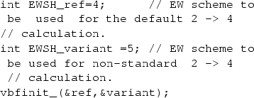
The EWSH_ref will set the initialization as used for the default calculation, and EWSH_variant for the reweighting with modified amplitudes. The choices 1, 2, 3, 4 correspond to EWSH=1, EWSH=2, EWSH=3, EWSH=4 respectively. The default EWSH=4, as explained in the main text, leads to correct \(\uptau \) lepton polarisations and angular distributions. As it causes at tree-level inconsistencies in the calculation of the WWZ coupling, we provide an additional option, EWSH=5, for which the parameter setting as for EWSH=4 is used, but with the WWZ coupling modified by 5 %. It can be used for testing sensitivity of the analysed distributions to the missed higher order corrections to the WWZ coupling. For more discussion, see Sect. 3.3.
-
PDFs and \({\varvec{\alpha }}_s\): Any PDF set from LHAPDF5 library [28] can be used for calculating weights. The choice can be configured by setting, string name=“cteq6ll.LHpdf”; LHAPDF::initPDFSetByName(name); The choice of renormalization and factorization scales (imposed is case of \(\mu _F=\mu _R\)) can be set with the help of the following command:
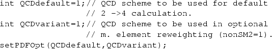
The choice can be different for the default (SM) calculation and the variant one (nonSM=true), see Appendix A.1, point 9. The \(Q^2\) evolution and starting value of \(\alpha _s\) used in PDF’s is internally defined by the LHAPDF5 library. For the matrix element calculations we do not impose consistent definition of \(\alpha _s\) but it can be enforced by the user, see the next point. As a default, we fix the starting point at \(\alpha _s(M_Z)=0.1180\) value and evolve it with \(Q^2\) with a simple formula of Eq. (4).
-
User own \({\varvec{\alpha }}_s\) in matrix element calculation: User can supersede the simple, leading logarithmic function provided by us for \(\alpha _s(Q^2)\) used in the matrix element calculation (Eq. (4)) with his preferred one, and pass it to the program. The function calculating \(\alpha _s\) has to have the following arguments: alphasModif(double Q2,int scalePDFOpt, int KEY) In alphasModif one can also use directly a method LHAPDF::alphasPDF(sqrt(Q2)) of LHAPDF5 library [28], the same assuring consistency between the value of \(\alpha _s\) in the matrix element and the structure functions. Such a function can be used by executing set_alphas Modif(alphasModif); . An example of such a setup has been provided in the example-VBF.cxx program.


1.3 A.3 Random number initialization
In most of the calculations the TauSpinner algorithms are not using random numbers. However, there are two exceptions. In both cases random generators from TAUOLA are used, see Appendix C.12 of Ref. [15].
-
The attribution of the helicity states uses Tauola::Ran domDouble. It should be replaced by the user, with the help of Tauola::setRandomGenerator(double (* gen)()) method and then properly initialized, with a distinct seed for each parallel run. In our example program the actual command is Tauola::setRandomGenerator( randomik );
-
If the read_particles_for_VBF.cxx code is required to generate \(\uptau \) decays, then a second random generator, coded in FORTRAN has to be also initialized with a distinct seed for each individual parallel run: Tauola::setSeed(int ijklin, int ntot in, int ntot2n).
1.4 A.4 Main program—an example
The following files are prepared for the user prototype program in the TAUOLA/TauSpinner/examples/examp le-VBF directory
-
The user example program example-VBF.cxx.
-
The prototype method read_particles_for_VBF. cxx to read in events stored in HepMC format is prepared specifically for MadGraph5 generated events.
-
The separate program lhef-to-hepmc.cxx for translating MadGraph5 events from the lhe [22] to HepMC [25] format.
-
The README file which contains auxiliary information.
Only the program example-VBF.cxx is generic, and does not depend on the specific environment for event generation. This is why we provide an extract from this code below. For the TauSpinner library to work, the \(\uptau \) decay products must be present in the event. In the case they are absent, like e.g. in events generated with \(\uptau \)’s as final states in MadGraph5, we prepared settings for their decays in the Tauola library using the mode of not-polarised \(\uptau \) decays of Tauola universal interface. Such additional processing is implemented in read_particles_for_VBF.cxx code.
In our demonstration program for TauSpinner spin correlations between \(\uptau \) leptons are then introduced, using \((2 \rightarrow 4)\) matrix elements and calculating the respective spin weight. The purpose of the example is to demonstrate the default initialisation of the TauSpinner program and a flow of the main event loop.
Extract from an example for main user program, example-VBF.cxx file.


1.5 A.5 New option for the \( (2 \rightarrow 2)\) case
We synchronize the old code for the \( (2 \rightarrow 2)\) processes with the method implemented for (\(2 \rightarrow 4\)) process TauSpinner::set_vbfdistrModif(vbfdistrMod if).
From now on, the first argument ID (passed by the TauSpinner library to the user-defined function nonSM_ado pt) denotes the incoming parton flavour PDGid. It is activated by the pointer: set_nonSM_born(nonSM_adopt) of /TAUOLA/TauSpinner/examples/tau-reweig ht-test.cxx.
In contrast, in earlier versions of TauSpinner library [8], it was possible to invoke user-defined function nonSM_adopt activated by the pointer in set_nonSM_born(nonSM_adopt). The first argument of this method was passing to the user function the information if incoming parton was up- or down-type quark only, without specifying its family affiliation.
B Tests of reweighting the differential cross-sections for Drell–Yan-like processes
In this Appendix we show in Figs. 9 and 10a complete set of kinematic distributions validating the implementation of (\(2 \rightarrow 4\)) non-Higgs Drell–Yan-like processes. We split \(pp \rightarrow \uptau \uptau jj\) events into four groups, depending on the initial partons, see Table 1 for definition of parton level processes. We use the implemented (\(2 \rightarrow 4\)) matrix elements to calculate per event a weight, \(wt_{prod}^{C \rightarrow D} = d\sigma _D/d\sigma _C\), see Eq. (6), defined as a ratio of the cross-sections for events of groups C and D. The expression is similar to Eq. (3) except that the sum is over subprocesses which belong to the chosen groups C or D. We apply \(wt_{prod}^{C \rightarrow D}\) to events from the group C and compare both the absolute normalisations and shapes of the re-weighted distributions with the distributions of events from the group D.
These tests were done on the large statistics samples and have been repeated between each groups of processes and within groups between subgroups. The achieved agreement between the reference and re-weighted distributions validates the correctness of the implemented matrix elements.

Shown are: the generated \(g\ q \rightarrow \uptau \uptau jj\) (thin red line), after reweighing to \( q\ q\ (qx\ qx) \rightarrow \uptau \uptau jj\) (red points). The reference \( q\ q\ (qx\ qx) \rightarrow \uptau \uptau jj\) distribution shown with a black line

Shown are: the generated \(g\ q \rightarrow \uptau \uptau jj\) (thin red line), after reweighting to \( q\ q\ (qx\ qx) \rightarrow \uptau \uptau jj\) (red points). The reference \( q\ q\ (qx\ qx) \rightarrow \uptau \uptau jj\) distribution shown with a black line
C Tests of reweighting differential cross-sections for Higgs boson production
Similar tests, as discussed in Appendix B, have been repeated for the \(pp \rightarrow H(\rightarrow \uptau \uptau ) jj\) processes. Results are shown in Figs. 11, 12, 13 and 14. Very good agreement between the reference and re-weighted distributions is observed, both for shapes and relative normalisations.

Shown is an example of test distributions for the generated process \(q\ q, qx\ qx \rightarrow H(\rightarrow \uptau \uptau ) jj\) (thin red line) after reweighting to \(q\ qx \rightarrow H(\rightarrow \uptau \uptau ) jj\) process (red points). The reference \(q\ qx \rightarrow H(\rightarrow \uptau \uptau ) jj\) distribution shown with a black line

Shown is an example of test distributions for generated process \(q\ q, qx\ qx \rightarrow H(\rightarrow \uptau \uptau ) jj\) (thin red line), after reweighting to \(q \ qx \rightarrow H(\rightarrow \uptau \uptau ) jj\) (red points). The reference \(q \ qx \rightarrow H(\rightarrow \uptau \uptau ) jj\) distribution shown with a black line

Shown is an example of tests distributions for generated process \(q\ qx \rightarrow H(\rightarrow \uptau \uptau ) jj\) (thin red line), after reweighting to \(q\ q, qx\ qx \rightarrow H(\rightarrow \uptau \uptau ) jj\) process (red points). The reference \(q\ q, qx\ qx \rightarrow H(\rightarrow \uptau \uptau ) jj\) distribution shown with a black line

Shown is an example of test distributions for the generated process \(q\ qx \rightarrow H(\rightarrow \uptau \uptau ) jj\) (thin red line), after reweighting to \(q \ q, qx\ qx \rightarrow H(\rightarrow \uptau \uptau ) jj\) (red points). The reference \(q\ q, qx\ qx \rightarrow H(\rightarrow \uptau \uptau ) jj\) distribution shown with a black line
D Optimalization of interface to Standard Model matrix element calculation
The steering function for calculating (\(2 \rightarrow 4\)) matrix elements squared REAL*8 FUNCTION VBFDISTR(ID1, ID2,ID3,ID4,HH1,HH2,PP,KEYIN) is coded in FORTRAN and stored in the VBF_distr.f file. Before invoking the calculation of particular matrix element squared of the Standard Model, it performs several steps of filtering to speed up the CPU needed for numerical calculations by setting matrix element squared to zero without calculation for the cases when configuration of partonic PDG identifiers for incoming and outgoing partons imply that it is the case. The following conditions are consecutively checked (strictly in the given order; in the case of non-standard calculations, these checks are not performed, because the function VBFDISTR is not invoked). Each condition must be passed to go to the next one, and finally to invoke the matrix element calculation.
Check if Matrix Element can be set to zero
-
1.
Two incoming (or two outgoing) parton identifiers correspond to gluons and the sum of the other two identifiers is zero, otherwise ID1 \( \cdot \) ID2 \(\cdot \) ID3 \(\cdot \) ID4 must be positive, to pass to the next step.
-
2.
mod(ID1 + ID2 + ID3 + ID4, 2) = 0,
-
3.
If both ID1,ID2 are negative or both ID3,ID4 are negative, and at least one of the other two ID’s is positive, then the result is zero.
-
4.
Charge conservation imposes that for processes without gluons the following condition must be fulfilled: mod(ID1,2) \( \cdot \) sign(ID1)+ mod(ID2,2) \( \cdot \) sign (ID2)=mod(ID3,2) \( \cdot \) sign(ID3) +mod(ID4,2) \(\cdot \) sign(ID4).
-
5.
The number of gluons in the process must be zero or two.
-
6.
If there are two gluons, then for the process to give a non zero contribution it is required that ID1 + ID2 = ID3 + ID4 or ID1 + ID2 =0 or ID3 + ID4 =0.
For some configurations it is enough to change the order of partons (arguments of VBFDISTR routine) or to apply the CP symmetry, to avoid duplicating routines for matrix element calculations. It is achieved by first copying kinematic variables into the local ones of VBFDISTR routine and then performing the following permutations/modifications of the parton positions and momenta:
Reorder arguments and apply the CP symmetry for a convenient choice of ID1, ID2
-
1.
For incoming quark-quark pair, we interchange the order, if necessary, to assure |ID1| \(\ge \) |ID2|.
-
2.
If all ID’s which do not correspond to gluons are negative, we change their signs. At the same time we interchange positions of \(\uptau ^+\) with \(\uptau ^-\) and flip signs of helicities. Finally we change signs of all 3-momenta to complete the CP transformation.
-
3.
For incoming quark–antiquark pair where at least one is non-first family, we require that |ID2| \(\le \) |ID1|. For the first family quarks we require that ID1=-1 or ID1=2 or |ID2|=|ID1|. To achieve that goal, if the condition is not fulfilled, we change the signs of all ID’s. At the same time we interchange positions of \(\uptau ^+\) with \(\uptau ^-\); their helicities signs are changed as well. Finally, we change signs of all 3-momenta to complete the CP transformation.
-
4.
We enforce (by reordering) that the first parton is not an antiquark, nor a gluon in the case of gluon-fermion initial state.
-
5.
If both ID1, ID2 are non gluon and positive, we enforce that ID1 \(\ge \) ID2
That completes transformations triggered by the configuration of identifiers of incoming partons. Note that if the third family is to be taken into account, also the sign of the CP symmetry breaking phase will have to be changed to complete the CP transformation.
Reorder arguments for a convenient choice of ID3, ID4
-
1.
The ID3 can not be negative and ID4 can not be alone the gluon.
-
2.
If both ID3 and ID4 are non-gluon and positive, then ID3 can be even and ID4 odd but not the other way.
-
3.
If both ID3 and ID4 are odd non-gluon and also ID3 \(\cdot \) ID4>0 , then ID4 must be larger/equal ID3.
-
4.
If ID3, ID4 are simultaneously even and also ID3 \(\cdot \) ID4>0, then ID4 must be larger/equal ID3.
Note that all of the above conditions are checked one after another. In particular, all necessary transformations (flipping the position of partons or invoking the CP transformation) are performed in the order as listed above. If all the above conditions are met, the matrix element is not set to zero and the order of arguments is adjusted to the available parton level routines, then numerical calculation of matrix element squared for a given helicity configuration, parton identifiers and momenta is performed.
Rights and permissions
Open Access This article is distributed under the terms of the Creative Commons Attribution 4.0 International License (http://creativecommons.org/licenses/by/4.0/), which permits unrestricted use, distribution, and reproduction in any medium, provided you give appropriate credit to the original author(s) and the source, provide a link to the Creative Commons license, and indicate if changes were made.
Funded by SCOAP3
About this article

Cite this article
Kalinowski, J., Kotlarski, W., Richter-Wa̧s, E. et al. Production of \(\uptau \) lepton pairs with high \(p_T\) jets at the LHC and the TauSpinner reweighting algorithm. Eur. Phys. J. C 76, 540 (2016). https://doi.org/10.1140/epjc/s10052-016-4361-9
Received:
Accepted:
Published:
DOI: https://doi.org/10.1140/epjc/s10052-016-4361-9