HistFitter software framework for statistical data analysis

Abstract

We present a software framework for statistical data analysis, called HistFitter, that has been used extensively by the ATLAS Collaboration to analyze big datasets originating from proton–proton collisions at the Large Hadron Collider at CERN. Since 2012 HistFitter has been the standard statistical tool in searches for supersymmetric particles performed by ATLAS. HistFitter is a programmable and flexible framework to build, book-keep, fit, interpret and present results of data models of nearly arbitrary complexity. Starting from an object-oriented configuration, defined by users, the framework builds probability density functions that are automatically fit to data and interpreted with statistical tests. Internally HistFitter uses the statistics packages RooStats and HistFactory. A key innovation of HistFitter is its design, which is rooted in analysis strategies of particle physics. The concepts of control, signal and validation regions are woven into its fabric. These are progressively treated with statistically rigorous built-in methods. Being capable of working with multiple models at once that describe the data, HistFitter introduces an additional level of abstraction that allows for easy bookkeeping, manipulation and testing of large collections of signal hypotheses. Finally, HistFitter provides a collection of tools to present results with publication quality style through a simple command-line interface.

1 Introduction

This paper describes a software framework for statistical data analysis, called “HistFitter”, that has been used extensively by the ATLAS Collaboration [1] to analyze big datasets originating from proton–proton collisions at the Large Hadron Collider (LHC) at CERN. Most notably, HistFitter has become a de facto standard in searches for supersymmetric particles since 2012, see for example [2–19], with some usage for Exotic [20, 21] and Higgs boson [22] physics. HistFitter is written in Python and C++, the former being used for configuration and the latter for CPU-intensive calculations. Internally, HistFitter uses the software packages HistFactory [23] and RooStats [24], which are based on RooFit [25] and ROOT [26, 27], to construct parametric models and perform statistical tests of the data. HistFitter extends these tools in four key areas:

• 1. Programmable framework: HistFitter performs complete statistical analyses of pre-formatted input data samples, from a single user-defined configuration file, by putting together tools from several sources in a coherent and programmable framework.

• 2. Analysis strategy: HistFitter has built-in concepts of control, signal and validation regions, which are used to constrain, extrapolate and validate models that describe that data, henceforth called “data models”, across an analysis. The framework also introduces a statistically rigorous treatment of the validation regions.

• 3. Bookkeeping: HistFitter can keep track of numerous data models, including all generated input histograms, both before and after adjustment to measured data, and can perform statistical tests and model-parameter scans of all these models in an organized way. This introduces a powerful additional level of abstraction, which aids the processing of large collections of signal hypothesis tests.

• 4. Presentation and interpretation: HistFitter provides a collection of methods to determine the statistical significance of signal hypotheses, estimate the quality of likelihood fits, and produce publication-quality tables and plots expressing these results.

This paper details these extensions and is organized as follows. Section 2 summarizes key concepts of the data analysis strategy used for many searches and measurements at the LHC, and which are ingrained in the HistFitter framework. Section 3 describes the central HistFitter configuration, the bookkeeping machinery, and the external statistics software packages that are steered. Section 4 describes the technical implementation of HistFitter, and how support for multiple Probability Density Function (PDF) instances of nearly arbitrary complexity has been implemented with a modular object-oriented design. Section 5 explains how the PDFs can be used to perform statistical fits¹ of various types. Section 6 describes how these fit results can be conveniently presented and visualized with different methods, for example for validation purposes. Finally, Sect. 7 explains the statistical formalism used, and shows how signal hypotheses can be tested quantitatively in several ways. The publicly available release of HistFitter is briefly described in Sect. 8, before concluding in Sect. 9.

2 Data analysis strategy

Particle physics experiments require the careful analysis of large data samples, coming from an experimental apparatus, in order to measure the properties of fundamental particles. A very active field of research is focused on using these datasets to discover physical processes that have been predicted by theoretical models, but have not yet been observed in nature.

Analyses generally rely on external predictions for the various background and signal components in the data to aid the interpretation of observations, where the signal component describes the process of interest. In particle physics, simulations of known and hypothesized physics processes are run through a detailed detector simulation, and are subsequently reconstructed with the same algorithms as the data. In addition, background samples can be constructed using data-driven methods. The simulated samples may depend on one or many model parameters, for example the masses of hypothesized new particles such as foreseen by supersymmetry. It may be required, for instance when signals are analyzed over a multi-dimensional space of model parameters, to sample from a “grid” of potential signal scenarios, with each point on that grid corresponding to a unique point in the multi-dimensional parameter space. If no excess is observed in the data, exclusion limits may be set within this grid, excluding a subset of the tested parameter values.

HistFitter configures and builds parametric models to describe the observed data, and provides tools to interpret the data in terms of these models. It uses the concepts of control, validation, and signal regions in the construction and handling of these models. A key innovation of HistFitter is to weave these concepts into its very fabric, and to treat them with statistically rigorous methods. The technical implementation of HistFitter is detailed in the following sections, where we explain two key ideas in data analysis strategy that have helped shape HistFitter.

2.1 Use of control, signal and validation regions

Any physics analysis aiming to study a specific phenomenon involves defining a region of phase space, obtained by applying selections to a set of kinematic observables, where a particular signal model predicts a significant excess of events over the predicted background level. Such a signal enriched region is called a signal region, or SR.

To estimate background processes contaminating the SR(s) in a semi-data-driven way, one typically defines control region(s), or CR(s), in which the dominant background(s) can be controlled by comparison to the data samples. CRs are specifically designed to have a high purity for one type of background, and should be free of signal contamination.

A third important component of data analysis is the validation of the model used to predict the number of background events in the SR(s). Validation region(s), VR(s), are defined for this purpose. VR(s) are typically placed in between the CR(s) and SR(s) in terms of selection criteria on the main kinematic observable(s) of the analysis. Hence, the choice of VR(s) is typically a trade-off between maximizing the statistical significance of the expected analysis result and minimizing signal contamination, while controlling the assumptions in the extrapolation from CR(s) to SR(s).

The concept of extrapolation between CRs, VRs and SRs is schematically shown in Fig. 1. Any such region can have one or many sub-regions, as illustrated by the dashed lines, where each sub-region is a histogram bin counting the number of events. The extrapolation happens in observables chosen to separate the regions, as discussed in Sect. 2.2, and shown by the arrows on the figure.

Fig. 1

A schematic view of an analysis strategy with multiple control, validation and signal regions. All regions can have single- or multiple bins, as illustrated by the dashed lines. The extrapolation from the control to the signal regions is verified in the validation regions that lie in the extrapolation phase space

To extract accurate and quantitative information from the data, particle physicists frequently use a Probability Density Function (PDF) whose parameters are adjusted with a fitting procedure. The fit to data is based on statistically independent CRs and SRs, which ensures that they can be modeled by separate PDFs and combined into a simultaneous fit. A crucial point of the HistFitter analysis strategy is the sharing of PDF parameters in all regions: CRs, SRs and VRs. This procedure enables the use of information from each signal and background component, as well as systematics uncertainties, consistently in all regions.

The analysis strategy flow is schematically shown in Fig. 2. If the dominant background processes are estimated with Monte Carlo (MC) simulations, their initial predictions are scaled to the observed event levels in the corresponding CRs, using normalization factors computed in the fit to data. Details on this fit follow in Sect. 5. Each such background sample has a single normalization factor, so the background predictions are scaled coherently in all regions, notably the SR(s). This results in so-called “normalized background predictions”, which are used to extrapolate into the VRs and SRs, as discussed in the next sub-section.

Fig. 2

Overview of a typical analysis strategy flow with HistFitter

2.2 Extrapolation and transfer factors

An underlying assumption has been made in the previous sections, that the kinematic variables are well modeled after fitting the PDF to the data, such that the extrapolation from CR(s) to SR(s) is valid. Once the dominant background processes have been normalized in the CR(s), the corresponding modifications to the PDF can be extrapolated to the VR(s), which is (are) then used to verify the validity of this assumption. In HistFitter, the PDF is coherently defined in all the CRs, SRs and VRs simultaneously, even though the VRs are never used as a constraint in the fit. This allows for a correct statistical extrapolation to the SRs and VRs, including any correlations between the fit parameters. Technical details on the extrapolation technique used in HistFitter are given in Sect. 5.2.

Once a satisfactory agreement is found between normalized background predictions and observed data in the VRs, the background predictions are further extrapolated to the SR(s), and, by convention, are only then compared with the observed data (see Fig. 2); a process generally called “unblinding” or “opening the box”. This ordering, of first validating the performance of the extrapolations, and, in a wider physics context, to get confidence in the methods used, avoids analyzers from using premature SR predictions, and thus potentially biasing the physics results.

A key underlying concept of the fitting procedure is the implicit use of ratios of expected event counts, called transfer factors, or TFs, for each simulated background process between each SR and CR. The normalized background predictions used in fit are:

$$\begin{aligned}&\begin{aligned}&N_p(\mathrm{CR}, \mathrm{est.}) = \mu _{p}\times \mathrm{MC}_p(\mathrm{CR},\mathrm{init.}) , \\&N_p(\mathrm{SR}, \mathrm{est.}) = \mu _{p}\times \mathrm{MC}_p(\mathrm{SR},\mathrm{init.}) , \end{aligned} \end{aligned}$$

(1)

where $N_p(\mathrm{CR}, \mathrm{est.})$ ($N_p(\mathrm{SR}, \mathrm{est.})$) is the CR (SR) background estimate for each simulated physics processes $p$ considered in the analysis, $\mathrm{MC}_p(\mathrm{CR}, \mathrm{init.})$ ($\mathrm{MC}_p(\mathrm{SR}, \mathrm{init.})$) is the initial estimate as obtained from the MC simulation, and $\mu _{p}$ is the normalization factor as obtained in the fit to data. In the fit, the background estimate(s) is (are) typically driven by the statistics in the CR(s). Define $N_p(\mathrm{CR}, \mathrm{fit})$ as the fitted number of events for process $p$ in the CR. Then equivalently:

$$\begin{aligned} N_p(\mathrm{SR}, \mathrm{est.})= & {} \mu _{p} \times \mathrm{MC}_p(\mathrm{SR},\mathrm{init.}) \nonumber \\\equiv & {} N_p(\mathrm{CR}, \mathrm{fit}) \times \left[ \frac{\mathrm{MC}_p(\mathrm{SR}, \mathrm{init.})}{\mathrm{MC}_p(\mathrm{CR}, \mathrm{init.})}\right] \,. \end{aligned}$$

(2)

The ratio appearing in the square brackets of Eq. 2 is defined as the transfer factor TF. The two notation are equivalent in terms of the fit: there is a normalization quantity, derived from the fit to data, multiplied by a fixed constant. In other words, albeit the fit uses Eq. 1 internally, $N_p(\mathrm{SR}, \mathrm{est.})$ can always be interpreted as a TF multiplied by the fitted number of background events in the CR.

An important feature of the TF approach is that systematic uncertainties on the predicted background processes can be (partially) canceled in the extrapolation; a virtue of the ratio of MC estimates. The total uncertainty on the number of background events in the SR is then a combination of the statistical uncertainties in the CR(s) and the residual systematic uncertainties of the extrapolation. For this reason, CRs are sometimes defined by somewhat loose selection criteria, in order to increase CR data event statistics without significantly increasing residual uncertainties in the TFs, which in turn reduces the extrapolation uncertainties to the SR.

3 HistFitter software framework

HistFitter provides a programmable framework to build and test a set of data models. To do so, HistFitter takes a user-defined configuration as input, together with MC simulation samples and the observed data. The HistFitter processing sequence then consists of three steps, illustrated by Fig. 3. From left to right:

• 1. Based on the user-defined configuration, HistFitter automatically prepares initial histograms, using ROOT, from the provided input source(s) that model the physics processes in the data. (The user-defined configuration and histogram creation is discussed further below and in Sect. 4.)

  Fig. 3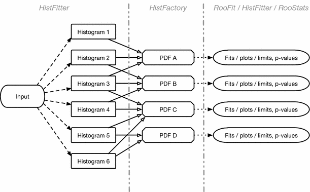

  

  Overview of the HistFitter processing sequence. Each column, separated by the dashed vertical lines, represents a step in the HistFitter processing sequence, and each row is a fit configuration. See the text for a description

• 2. According to each specified configuration, e.g. including or excluding the VR(s), the generated histograms are combined by HistFactory to construct a corresponding PDF. At the end of this process, each PDF is stored together with the observed dataset.

• 3. The constructed PDFs are used to perform fits of the data with RooFit, perform statistical test with RooStats, and to produce plots and tables.

These steps all require a substantial bookkeeping and configuration machinery, which is provided by HistFitter. The following sub-sections summarize the central HistFitter configuration and the prominent features of the HistFactory and RooStats software tools that HistFitter utilizes.

3.1 Configuration and steering

The various steps of Fig. 3 can be executed individually or consecutively in a single run, and are all controlled with a single (and simple) user-defined configuration file. For example, in early stages of an analysis selection criteria may need to be determined, requiring frequent regeneration of just the histograms that describe the data. Whereas, when moving to later stages in an analysis, allowing one to go straight to e.g. the statistical significance determination of the analysis result can have quite a beneficial impact.

One of the key benefits of having a single configuration is to aid collaboration between the various members of an analysis group. The ability to rerun an analysis reasonably quickly, as long as the histograms have been created, helps tremendously in sharing workload between a collaboration, as does having the statistical tools easily accessible to the various members of an analysis group. Likewise, the process of combining existing analyses is made more efficient than if each group has to submit histograms independently to some third party for a statistical combination.

The central HistFitter configuration and bookkeeping machinery is built around a configuration manager. When executing HistFitter, users interact with the configuration manager to define a number of so-called fit configurations. (The technical implementations of these objects are described in Sect. 4.) A fit configuration describes the configuration of all processing steps of Fig. 3: it contains a PDF describing the CR, SR and VR data belonging to that fit configuration, together with meta-data required for the sequence of building, fitting, visualizing and interpreting each configuration, including the generation of all relevant input histograms.

The construction of each data model typically requires the preparation of tens to hundreds of histograms. This can lead to memory exhaustion problems for long lists of models. However, while signal samples tend to be unique to each model, the background samples are often identical in most of the models. When preparing input histograms for each sample of each model, the configuration manager stores unique auto-generated names in a dictionary. The dictionary is used in turn to identify and re-use the histograms that can be shared between independent data models (see Fig. 3), which significantly reduces the memory usage of the software. Additionally, the generated histograms are stored in an external file, allowing them to be directly loaded when rerunning HistFitter in the same configuration. This avoids the need for their, usually time-consuming, regeneration, and helps in sharing workload between a collaboration.

3.2 HistFactory

HistFitter uses the HistFactory package to construct a parametric model² describing the data, based on provided input histograms. This parametric model describes the nominal, i.e. preferred, prediction together with associated systematic variations of multiple signal and background processes in multiple regions, up to nearly arbitrary complexity. The input histograms can be generated by HistFitter, or can be provided externally by users.

As detailed in Ref. [23], the PDF constructed by HistFactory contains the parameter(s) of interest, such as the rate of a signal process, the normalization factors for background processes (as estimated from the data), and the so-called nuisance parameters that model the impact of systematic uncertainties. Each systematic uncertainty $i$ is described with a nuisance parameter, $\theta _i$, that continuously interpolates between the nominal and (systematic uncertainty) variation templates, e.g. $\theta _i=\pm 1$ for $\pm 1\sigma$ variations of the systematic uncertainty, and $\theta _i=0$ for the nominal template, where $1\sigma$ means one standard deviation.

The general likelihood $L$ of the event-counting analyses considered here is the product of Poisson distributions of event counts in the SR(s) and/or CR(s) and of additional distributions that implement the constraints on systematic uncertainties. It can be written as:

$$\begin{aligned} L({\varvec{n}},\varvec{\theta }^0|\mu _\mathrm{sig},{\varvec{\mu }_p},{\varvec{\theta }})= & {} \mathcal {P}_\text {SR} \;\times \; \mathcal {P}_\text {CR} \;\times \; \mathcal {C}_\text {syst} \nonumber \\= & {} \prod _{i\in \text {SR}} P(n_{i}|\lambda _{i}(\mu _\mathrm{sig},{\varvec{\mu }_p,\varvec{\theta }})) \nonumber \\&\quad \times \prod _{i\in \text {CR}} P(n_{i}|\lambda _{i}(\mu _\mathrm{sig},{\varvec{\mu }_p,\varvec{\theta }})) \nonumber \\&\quad \times \, C_\text {syst}(\varvec{\theta }^0,\varvec{\theta }) \,. \end{aligned}$$

(3)

The first two factors of Eq. 3 ($\mathcal {P}_\text {SR}$ and $\mathcal {P}_\text {CR}$) reflect the Poisson distributions, $P$, of $n_{i}$, which is the number of observed events in each signal and control region bin $i$. The Poisson expectations $\lambda _i$ are functions depending on the predictions for the signal and various background sources $p$, the nuisance parameters that parametrize systematic uncertainties, $\varvec{\theta }$, the normalization factors for background processes, $\varvec{\mu }_{p}$, and also the signal strength parameter $\mu _\mathrm{sig}$. ($\mu _{p}$ is the same parameter as in Eq. 1.) For $\mu _\mathrm{sig}=0$ the signal component is turned off, and for $\mu _\mathrm{sig}=1$ the signal expectation equals the nominal value of the model under consideration.

The predictions for signal and background sources are forced to be positive in HistFactory for any values of the nuisance parameters and in any histogram bin.

Systematic uncertainties are included using the probability density function $C_\text {syst}(\varvec{\theta }^0,\varvec{\theta })$, where $\varvec{\theta }^0$ are the central values of the auxiliary measurements around which $\varvec{\theta }$ can be varied, for example when maximizing the likelihood. The impact of changes in nuisance parameters on the expectation values are described completely by the functions predicting the amount of signal and background, $\lambda _{S}$ and $\lambda _{i}$. For independent nuisance parameters, $C_\text {syst}$ is simply a product of the probability distributions corresponding to the auxiliary measurements describing each of the systematic uncertainties, typically Gaussians $G$ with unit width,

$$\begin{aligned} C_\text {syst}(\varvec{\theta }^0,\varvec{\theta }) = \prod _{j\in \text {S}} G(\theta _\text {j}^0-\theta _\text {j}), \end{aligned}$$

(4)

where S is the full set of systematic uncertainties considered. The auxiliary measurements $\theta _\text {j}^0$ are typically fixed to zero, but can be varied when generating pseudo experiments (see below).

Several interpolation (and extrapolation) algorithms are employed in HistFactory to describe the PDF for all values of nuisance parameters $\theta _\text {j}$. For a complete overview the reader is referred to Ref. [23].

The execution of HistFactory results in a a persistable RooFit object containing the parametrized PDF, the dataset, and a helper object summarizing the model configuration (used for the statistical interpretation). These are used as input to perform statistical tests with the RooStats package, as discussed in the next sub-section.

3.3 RooStats

HistFitter is capable of performing a list of pre-configured statistical tests to one or several dataset(s) from a single command-line call. To do so, it interfaces with the RooStats package. These tests are:

• 1. hypothesis tests of signal models;

• 2. the construction of expected and observed confidence intervals on model parameters. For example, the 95 % confidence level upper limit on the rate of a signal process;

• 3. the significance determination of a potentially excess of observed over expected events in a signal region.

A suite of statistical calculations can be performed, as configured by the user, ranging from Bayesian to Frequentist philosophies and using various test statistic quantities as input.³ By default, HistFitter employs a Frequentist method to perform hypothesis tests and uses the profile likelihood ratio $q_{\mu _\mathrm{sig}}$ as test statistic. The CLs method [28] is used to test the exclusion of new physics hypothesis. Whenever appropriate, this method is approximated by asymptotic formulae [29] to speed up the evaluation process.

More details about how hypothesis tests are performed with HistFitter are given in Sect. 7.

4 Programming of probability density functions

HistFitter is designed to build and manipulate PDFs of nearly arbitrary complexity.

In the terminology of HistFactory, the likelihood function in Eq. 3 has multiple channels, which need inputs in the form of samples, corresponding to the signal and background processes for that region. In turn, the various samples have systematic uncertainties, or systematics. A HistFactory “channel” is a synonym for a “region”, generically referring to either CR, SR or VR in this section. The systematic uncertainties can be either statistical, theoretical or experimental in nature. These HistFactory C++ classes are mirrored (overloaded) by HistFitter in Python, and extended by adding the flexibility to construct multiple PDFs from these building blocks in a programmable way.

The technical components to do this are discussed in this section, which follows a top-to-bottom description of the classes illustrated in Figs. 4 and 5.

Fig. 4

Illustration of a fit configuration in HistFitter. Each fitConfig instance defines a PDF built from a list of channel (i.e. CR, SR or VR), sample and systematic objects. Each channel owns a list of samples and each sample owns a list of systematic uncertainties. Correlated samples and systematics are declared by being given identical names. Otherwise they are treated as un-correlated

Fig. 5

The methods addChannel(), addSample() and addSystematic() are used to build complex PDFs in an intuitive way. The methods addSample and addSystematic implement a “trickle down” mechanism, discussed in the text

4.1 The configuration manager

The HistFitter configuration and bookkeeping machinery is built around a central configuration manager, config Manager, implemented by two singleton objects: one in Python and one in C++. When executing HistFitter, users interact with the Python interface of the configManager to define, for each data model, a fitConfig object, describing the fit configuration.

The fitConfig class configures each processing step of Fig. 3; it is described below in Sect. 4.2. The configuration manager can hold any number of fitConfig objects.

In terms of design patterns, the configManager can be seen as a “factory of factories”, since it generates the fitConfig objects that are themselves factories of PDF objects. By producing a list of data models, HistFitter thus introduces an additional level of abstraction which allows hypothesis tests to be performed over sets of signal models.

4.2 The fit configuration

HistFitter uses the fitConfig class to construct its PDFs. The design of this class allows for the creation of highly complex PDFs, describing highly non-trivial analysis setups, with only a few lines of intuitive code.

This is configured by users as follows:

where myFitConfig is a reference to a new fitConfig object owned by the configManager. The fitConfig class logically corresponds to a PDF decorated with meta-data about the properties of the contained channels (CR, SR, VR), including visualization, fitting and interpretation options.

During configuration, instances of channels, samples and systematics are put together by fitConfig objects, together with links to the corresponding input histograms. During execution, the fitConfig information is used to steer the HistFactory package’s creation of a RooSimultaneous object modelling the actual PDF with RooFit.

Figure 4 illustrates the modular design of a typical HistFitter fit configuration. The user interface provides the methods addChannel(), addSample() and addSystematic () to build up data models in an intuitive manner. For instance, samples and systematics can be efficiently added to multiple channels through a “trickle-down” mechanism, as illustrated by Fig. 5. This means that fitConfig.addSample () adds a sample to all the channels owned by the fitConfig, while channel.addSample() adds a sample to one specific channel. Similarly, sample.addSystematic() only adds a systematic to one specific sample while channel.addSystematic() adds a systematic to all the samples owned by the channel and fitConfig.add Systematic() adds a systematic to all the samples of all the channels owned by the fitConfig.

Since different channels often share the same samples (i.e., processes), and different samples often share the correlated systematic uncertainties, the trickle-down mechanism is in fact an extremely useful feature. This ensures that complex configurations of PDFs can often be described with only a few lines of code. As illustrated in Fig. 5, one simply adds all channels, samples, and systematic uncertainties directly to the fitConfig object and lets these “trickle down”, thereby automatically creating a highly advanced fit configuration.

A basic fit configuration can also be conveniently cloned and extended to specify new configurations, a feature which is frequently used to build data models corresponding to multiple signal hypotheses from a common background description.

4.3 Channels

The Channel objects contain data from a region of phase space defined by event selection criteria on the input dataset. Channels can represent either a simple event count (i.e. one bin), or the multi-binned distribution of a physical observable. New binned and un-binned channels can be added to a fitConfig by calling:

where myObs is the name of an element of the input dataset, nBins, varLow and varHigh indicate the number of bins and the range of values as for a one-dimensional histogram, and mySelection specifies the selection criteria of the considered region. For un-binned channels, cuts is a reserved keyword indicating that only the total the number of events passing the selection criteria needs to be considered.⁴

A Channel object can represent a CR, SR or VR. This information is configured by users as follows:

It is possible to add an arbitrary number of channels to a given fitConfig by simply calling addChannel() multiple times. Consequently, HistFitter automatically performs simultaneous fits constrained by the data of all BkgConstrainChannels (CR) and SignalChannels (SR), but not by the ValidationChannels (VR). The data itself is described by a list of Sample objects owned by each channel, as discussed in the next sub-section.

4.4 Samples

The Sample class logically corresponds to a component of a RooFit PDF decorated with HistFitter meta-data. In a typical particle physics analysis, each sample corresponds to a specific physics process and several samples are needed to model a complete dataset.

In HistFitter, samples can be defined in a specific channel or defined simultaneously in multiple channels. The Sample class also owns a list of objects representing its systematic uncertainties. Importantly, samples provide the link between input data and the respective components of the PDF. Three types of inputs are supported:

• 1. TTree: a ROOT data structure, stored in a TFile, in which a list of events is mapped to a list of key-value pairs characterizing the properties of each event;

• 2. Float: floating point numbers provided by users through the Python interface of HistFitter;

• 3. Histogram: pre-made histograms using the ROOT TH1 data structure, stored in an external TFile.

The most commonly used type of input is TTree, which provides maximal flexibility and features but requires the largest amount of processing power and disk I/O. Float inputs tend to be used for quick tests and simple processes. Histogram inputs can be used for compatibility with external frameworks, and also allow the user to conveniently skip the TTree-to-histogram processing when re-building PDFs. In all cases, the initial input is transformed into histograms as specified by Sample objects, before being saved to a temporary file and passed to HistFactory to build the RooFit PDFs (see Sect. 4.2).

A basic sample can be created and configured by users as follows:

which constructs a sample object owned by myChannel and displayed with myColor color by the visualization tools. In this example, HistFitter takes inputs from a TTree object named SampleName in the default ROOT file specified at the configManager level. To construct the sample, HistFitter uses the event selection criteria of the parent channel and applies a default sample weight.

The default settings can be over-written by users to achieve specific goals. For instance, a sample can be built from Float input with:

where the list [100,34,220] specifies the bin content of three bins in an histogram. The default sample weight and path to the input data can also be over-written as follows:

Weights are passed as a string to also allow the easy use of weights stored in a ROOT TTree. In addition, the Sample class has optional methods to configure its corresponding RooFit PDF, such as:

resulting in the deactivation (activated by default) of built-in Poisson statistical uncertainties, and in the creation of a fit normalization factor my_Norm with initial value 1.0 and allowed range 0.0 to 10.0, respectively.

Last but not least, HistFitter provides many features for modeling the systematic uncertainties associated to each sample, as discussed in the next sub-section.

4.5 Systematic uncertainties

For each component of the PDF, a nominal distribution representing the best available prediction is typically provided to the physics analysis as a histogram owned by a Sample object. These components typically have systematic uncertainties whose impact gets quantified in dedicated studies. This is often modeled as variations of one standard deviation around the nominal prediction, provided to the physics analysis as sets of two additional histograms. These systematic uncertainties are parametrized in the PDF with nuisance parameters, as in Eq. 3.

In HistFitter, systematic uncertainties are implemented with a dedicated Systematic class with several options. In a typical analysis, several Systematic objects are built and owned by a parent Sample. Through the trickle down mechanism described in Sect. 4, systematics can be defined for a specific sample or defined simultaneously for multiple samples and/or multiple channels.

A Systematic object can be conceived as a doublet of samples specifying up and down variations around the parent Sample. Hence Systematic objects can be constructed from the same types of inputs as Samples, namely: TTree, Float and histogram.

When using TTree inputs, two methods can be used to compute the up/down variations of a systematic: weight-based or tree-based. In the weight-based method, histograms are always built from the same TTree, using three different sets of weights: up, nominal and down. In the tree-based method, histograms are built from three different TTrees using the same set of weights. If only one variation is available, users can either build a one-sided uncertainty or symmetrize the variation as $\mathrm {\frac{nominal\, \pm \, (up-nominal)}{nominal}}$.

Systematic objects can be created by users as follows:

where myTreeSys and myWeightSys rely on the tree-based and weight-based methods. myUserSys relies on the Float input discussed above, and, in this example, has asymmetric up and down input uncertainty values of 10 and 20 %. The last argument myMethods is discussed below. Systematic objects are then associated to Sample or Channel objects with:

As illustrated in Fig. 4, correlated systematic uncertainties are declared simply by giving them identical names in the corresponding Samples. Otherwise they are treated as uncorrelated.

When turning the above into nuisance parameters, additional input is required to specify the interpolation (extrapolation) algorithm and constraint parametrization for each systematic uncertainty. This is done with the argument myMethods above. Several possible analysis strategies can be envisaged, requiring a detailed discussion, case by case. To address this, HistFitter does not enforce a specific strategy but provides users with as many methods as possible to cover all reasonable possibilities.

The basic methods for systematic uncertainties defined in HistFactory are called: overallSys, histoSys and shapeSys, and are listed in the top half of Table 1.

Table 1 Sub-set of the systematic methods available in HistFitter. The methods are specified by a string argument containing a combination of basic HistFactory methods and optional HistFitter keywords: norm, OneSide and/or Sym. Systematic objects can be built with Tree-based, weight-based, Float or histogram input methods in all cases

An overallSys describes an uncertainty of the global normalization of the sample. This method does not affect the shape of the distributions of the sample. A histoSys describes a correlated uncertainty of the shape and normalization. Both methods use a Gaussian constraint to model an uncertainty and allow for asymmetric uncertainties, simply by providing asymmetric input values or histograms. By default they are configured to use a 6th-order polynomial interpolation technique between the $\pm 1 \sigma$ and nominal histograms and a linear extrapolation beyond $|1\sigma |$ [23], though they can be configured differently.

A shapeSys describes an uncertainty of statistical nature, typically arising from limited MC statistics. In HistFactory, shapeSys is modeled with an independent parameter for each bin of each channel. It is shared between all samples of that channel with StatConfig==True (see Sect. 4.3). For simplicity, users can also set a threshold below which samples are neglected when building a shapeSys. The interpolation and extrapolation technique used for shapeSys are as for histoSys, and parametrized as a Poissonian constraint.

To respond to various use cases encountered during real-life analysis of ATLAS Run-1 data, HistFitter provides additional systematic methods derived from the basic HistFactory methods. A sub-set of the systematic methods available in HistFitter is listed in the bottom half of Table 1.

These methods can be specified with combinations of the norm, OneSide and Sym keywords. The norm keyword indicates that the total event count is required to remain invariant in a user-specified list of normalization region(s) when constructing up/down variations. This describes uncertainties of the shape only. Such a systematic uncertainty is transformed from an uncertainty on event counts in each region into a systematic uncertainty on the transfer factors, as discussed in Sect. 2 (Eq. 2). The OneSide and Sym keywords indicate that a one-sided or a symmetrized uncertainty should be constructed when using tree-based or weight-based inputs.

5 Performing fits

Different fit strategies are commonly used in physics analyses, differing by the usage of particular combinations of CRs, SRs, and VRs, and by the consideration of a signal model or not. Fit strategies aim to either derive background estimates in VRs and SRs, or to make quantitative statements on the compatibility of the background estimate(s) with the observed data in the SR(s). HistFitter is tailored specifically to the design and implementation of such fit strategies.

Also discussed in this section are the technical and statistical details of the extrapolation of background processes across CRs, SRs and VRs.

5.1 Common fit strategies

The three most commonly used fit strategies in HistFitter are defined as: the “background-only fit”; the “model-dependent signal fit”; and the “model-independent signal fit”.⁵ This section describes the details of each fit strategy, as also summarized in Table 2 at the end of the section. The application of these to validation and hypothesis-testing purposes is described in detail in Sects. 6 and 7, respectively.

5.1.1 Background-only fit

The purpose of this fit strategy is to estimate the total background in SRs and VRs, without making assumptions on any signal model. As the name suggests, only background samples are used in the model. The CRs are assumed to be free of signal contamination. The fit is only performed in the CR(s), and the dominant background processes are normalized to the observed event counts in these regions. The maximized likelihood function is that of Eq. 3 minus the signal regions. As the background parameters of the PDF are shared in all different regions, the result of this fit can be used to predict the number of events in the SRs and VRs.

The background predictions from the background-only fit are independent of the observed number of events in each SR and VR, as only the CR(s) are used in the fit. This allows for an unbiased comparison between the predicted and observed number of events in each region. In Sect. 6 the background-only fit predictions are used to validate the transfer factor-based background level predictions.

Another important use case for background-only fit results in the SR(s) is for external groups to perform an hypothesis test on an untested signal model, which has not been studied by the experiment. With the complex fits currently performed at the LHC, it may be difficult (if not impossible) for outsiders to reconstruct these. An independent background estimate in the SR, as provided by the background-only fit, is then the correct estimate to use as input to any hypothesis test.

For completeness we also introduce the concept of background-level estimates obtained from a background-only fit in both the CRs and SRs.⁶ The RooStats routines employed in HistFitter perform such a background only fit internally, before running any hypothesis testing; discussed further in Sect. 7. However, unless indicated explicitly, any background-level prediction made by HistFitter does not rely on SR (or VR) information.

Table 2 Summary of the fit strategies supported in HistFitter, as described in the text

5.1.2 Model-dependent signal fit

This fit strategy is used with the objective of studying a specific signal model. In the absence of a significant event excess in the SR(s), as concluded with the background-only fit configuration, exclusion limits can be set on the signal models under study. In case of excess, the model-dependent signal fit can be used to measure properties such as the signal strength. The fit is performed in the CRs and SRs simultaneously. Along with the background samples, a signal sample is included in all regions, not just the SR(s), to correctly account for possible signal contamination in the CRs. A normalization factor, the signal strength parameter $\mu _\mathrm{sig}$, is assigned to the signal sample.

Note that this fit strategy can be run with multiple SRs (and CRs) simultaneously, as long as these are statistically independent, non-overlapping regions. If multiple SRs are sensitive to the same signal model, performing the model-dependent signal fit on the statistical combination of these regions shall, in general, give better (or equal) exclusion sensitivity than obtained in the individual analyses. An example of this is given in Fig. 10 (right) of Sect. 7.2.

In a similar fashion, using multiple bins of a signal-sensitive observable in the definition of the SR(s) will generally give a better sensitivity to any signal model studied.⁷ An example of such a “shape-fit” signal region is shown in Fig. 8 of Sect. 6.1.

Typically, a grid of signal samples for a particular signal model is produced by varying some of the model parameters, e.g. the masses of predicted particles. The model-dependent signal fit is repeated for each of these grid points, thereby probing the phase space of the model. Examples of this are provided in Sects. 7.2 and 7.3.

5.1.3 Model-independent signal fit

An analysis searching for new physics phenomena typically sets model-independent upper limits on the number of signal events on top of the expected number of background events in each SR. In this way, for any signal model of interest, anyone can estimate the number of signal events predicted in a particular signal region and check if the model has been excluded by current measurements or not.

Setting the upper limit is accomplished by performing a model-independent signal fit. For this fit strategy, both the CRs and SRs are used, in the same manner as for the model-dependent signal fit. Signal contamination is not allowed in the CRs, but no other assumptions are made for the signal model, also called a “dummy signal” prediction. The SR in this fit configuration is constructed as a single-bin region, since having more bins requires assumptions on the signal spread over these bins. The number of signal events in the signal region is added as a parameter to the fit. Otherwise, the fit proceeds in the same way as the model-dependent signal fit.

The model-independent signal fit strategy, fitting both the CRs and each SR, is also used to perform the background-only hypothesis test, which quantifies the significance of any observed excess of events in a SR, again in a manner that is independent of any particular signal model. One main but subtle difference between the model-independent signal hypothesis test (Sect. 7.4) and the background-only hypothesis test (Sect. 7.5) is that the signal strength parameter is set to one or zero in the profile likelihood numerator respectively.

5.2 Extrapolation and error propagation

This section discusses the extrapolation of coherently normalized background estimates from the CR(s) to each SR and VR, as obtained from the background-only fit.⁸

The basic strategy behind the background extrapolation approach is to share the background parameters of the PDF in all the different regions: CRs, SRs and VRs. A background-only fit to the CRs technically requires a PDF modeling only the CRs. However, the extrapolation of the normalized background processes from the CRs to the SRs and VRs, which uses the background-only fit result, requires a different PDF containing all these regions.

In HistFitter, the construction of these various PDFs proceeds as follows. First a total PDF describing all CRs, SRs and VRs is constructed using HistFactory. This PDF is not used to fit the data, as the likelihood is unaware of the concept of different region types. HistFitter has dedicated functions to deconstruct and reconstruct PDFs, based on the channel type information of CR, VR and SR set in the configuration file, as discussed in Sect. 4.3.

To perform the background-only fit, the total PDF is deconstructed and then reconstructed describing only the CRs. The result of the background-only fit is stored, containing the values, the errors and the covariance matrix corresponding to all fit parameters. After this fit, the normalized backgrounds are extrapolated to the SRs (or VRs). For this HistFitter deconstructs and reconstructs the total PDF, now describing the CRs and SRs (or VRs). The background-only fit result is then incorporated into this PDF to obtain the extrapolated background prediction $b$ in any SR (or VR).

Once the background-only fit to data has been performed and the total PDF been reconstructed, an estimate of the uncertainty on an extrapolated background prediction $\sigma _{b,\,tot}$ can be calculated. The determination of this error requires the uncertainties and correlations from the stored fit result. The total error on $b$ is calculated using the typical error propagation formula

$$\begin{aligned} \sigma _{b,\,tot}^2 = \sum \limits _{i}^n \bigg (\frac{\partial b}{\partial \eta _i}\bigg )^2 \sigma ^2_{\eta _i} + \sum \limits _{i}^n \sum \limits _{j\ne i}^n \rho _{ij} \bigg (\frac{\partial b}{\partial \eta _i}\bigg ) \bigg (\frac{\partial b}{\partial \eta _j}\bigg ) \sigma _{ \eta _i}\sigma _{ \eta _j}, \end{aligned}$$

(5)

where $\eta _{i}$ are the floating fit parameters, consisting of normalization factors $\varvec{\mu _p}$ and nuisance parameters $\varvec{\theta }$, $\rho _{ij}$ is the correlation coefficient, between $\eta _{i}$ and $\eta _{j}$, and $\sigma _{\eta _i}$ is the standard deviation of $\eta _i$. Any partial derivatives to $b$ are evaluated on the fly.

The after-fit parameter values, errors and correlations are saved in the RooFit’s fit result class. Let us take an example of a background-only fit result (from CRs only) that needs to be extrapolated to a SR. The total PDF (consisting of CRs and SRs) contains a set of parameters that can be subdivided as follows.

• 1. There is a large set of parameters shared between CRs and SR, ${\varvec{\eta }}_{\mathrm {shared}}$, for example the background normalization factors and most systematic uncertainties.

• 2. There is a subset of parameters connected only to the CRs, ${\varvec{\eta }}_{\mathrm {CR}}$, for example the uncertainties due to limited Monte Carlo statistics in the CRs.

• 3. And finally, there is another subset of parameters connected only to the SR, ${\varvec{\eta }}_{\mathrm {SR}}$, for example the uncertainties due to limited Monte Carlo statistics in the SR.

When the fit is performed with the (deconstructed) CRs-only PDF, only the parameters ${\varvec{\eta }}_{\mathrm {shared}}$ and ${\varvec{\eta }}_{\mathrm {CR}}$ are evaluated and saved in the fit result.

Hence when this fit result is propagated to the SR, the estimated error only contains the parameters that are shared between the CRs and the SR, and thus is incomplete. The uncertainties corresponding to ${\varvec{\eta }}_{\mathrm {SR}}$ are not picked up in Eq. 5, as these are not contained in the fit result.

HistFitter uses an expanded version of RooFit’s fit result class that contains all of the nuisance parameters of all regions in the extrapolation PDF, even if these are not used in the background-only fit configuration. This expansion makes it possible to extrapolate all of the shared parameters to any region. Knowing also the unshared parameters of a particular region, a complete error can then be calculated for that region. In the expanded fit result, the correlations between the shared and unshared parameters are set to zero.

Using the expanded fit result class the VRs can now provide a rigorous statistical cross check. If the background-only fit to the CRs finds that changing the background normalization and/or shape parameters of a kinematic distribution gives a better description of the data, this will be reflected automatically in the VRs. Likewise, if the uncertainty on these parameters has a strong impact, and is reduced by the fit, the effect will be readily propagated.

In HistFitter, the before-fit parameter values, errors and correlations are stored in an expanded fit result object as well. The before-fit and after-fit background value and uncertainty predictions can thus be easily compared. A few assumptions are made to construct this before-fit object. First, all correlations are set to zero prior to the fit, effectively taking out the second term in Eq. 5. Second, the errors on the normalization factors of the background processes are unknown prior to the fit, and hence set to zero.

The fit strategies of Sect. 5.1 are illustrated in Fig. 6, together with the PDF restructuring detailed in this section. In Fig. 6, the various constructed PDFs are indicated as rounded squares and the fit configurations, on the right-hand side, as squares.

Fig. 6

An overview of the various PDFs HistFitter uses internally, together with their typical use. The large PDF for all regions is automatically deconstructed into separate, smaller ones defined on those subsets of regions depending on the fit and/or statistical test performed. The PDFs are indicated as rounded squares, and the fit configurations as squares

6 Presentation of results

HistFitter contains an extensive array of user-friendly functions and scripts, which help to understand in detail the results obtained from the fits. All scripts and plotting functions can be called by single-line commands. These scripts and plotting functions are generalized, and work for each model built with HistFitter.

Two main presentation components are the visualization of fit results and scripts for producing event yield and uncertainty tables. Both rely critically on the fits to data and uncertainty extrapolation features discussed in Sect. 5. All tables and plots, discussed in the next two sections, can be produced for any fit configuration of a defined model, as well as before and after the fit to the data. Multiple details, such as the legends on plots or the set of regions to be processed for tables, can be set in the configuration file or from the command line.

All tables and figures shown in this section come directly from publications by the ATLAS collaboration, and serve only as illustrations of the HistFitter tools that are discussed.

6.1 Visualization of fit results

HistFitter can produce several classes of figures to visualize fit results, as detailed below.

Figure 7 shows an example plot of a multi-bin (control) region before (left) and after (right) the fit to the data, taken from Ref. [2]. Similar plots can be produced for any region defined in HistFitter, either single- or multi-binned. Each sample in the example region (channel) is portrayed by a different color. The samples can also be plotted separately (not shown), for the purpose of understanding the distribution of the uncertainties over the samples. The impact of the fit to data can be studied by comparing the before-fit to after-fit distributions. In the after-fit plot, as a result of the fit, the normalization, shapes and corresponding uncertainties of the background samples have been adjusted to best describe the observed data over all bins.

Fig. 7

Example produced by the ATLAS collaboration and taken from Ref. [2]. Distribution of missing transverse momentum in the single lepton $W$+jets control region before (top) and after (bottom) the final fit to all background control regions

An example of two multi-binned SRs, used in Ref. [19], is shown in Fig. 8. Two different supersymmetry models, showing strong variations in the event yields over the bins of the SRs, are superimposed on the before-fit background predictions.

Fig. 8

Example produced by the ATLAS collaboration and taken from Ref. [19]. Effective mass distributions in the signal regions SR0b and SR1b, used as input for model-dependent signal fits. For illustration, predictions are shown from two SUSY signal models with particular sensitivity in each signal region

Figure 9 shows an example of a pull distribution for a set of non-overlapping VRs, as produced with HistFitter and taken from Ref. [2]. The example relies on the background prediction in each VR, as obtained from a fit to the CRs, and tests the validity of the transfer-factor based extrapolation. The pull $\chi$ is calculated as the difference between the observed $n_\mathrm{obs}$ and predicted event numbers $n_\mathrm{pred}$, divided by the total systematic uncertainty on the background prediction, $\sigma _\mathrm{pred}$, added in quadrature to the Poissonian variation on the expected number of background events, $\sigma _\mathrm{stat,\,exp}$.

$$\begin{aligned}&\chi = \frac{n_\mathrm{obs} - n_\mathrm{pred}}{\sigma _\mathrm{tot}} \end{aligned}$$

(6)

$$\begin{aligned}&\sigma _\mathrm{tot} = \sqrt{\sigma _\mathrm{pred}^2 + \sigma _\mathrm{stat,\,exp}^2} \end{aligned}$$

(7)

If, on average, the pulls for all the validation regions would be negative (positive), the data is overestimated (underestimated) and the model needs to be corrected. If the background model is properly tuned, on average good agreement is found between the data and the estimated background model.

Fig. 9

Example produced by the ATLAS collaboration and taken from Ref. [2]. Summary of the fit results in the validation regions. The difference between the observed and predicted number, divided by the total (statistical and systematic) uncertainty on the prediction, is shown for each validation region

Other validation plots can be produced, mostly helpful for internal or debugging purposes. Likelihood scans can be made for any of the fit parameters to help understand the likelihood maximization performed in the fit. Furthermore, the correlation matrix of any fit can be plotted to study correlations between the fit parameters and possible degenerate degrees of freedom. Those examples are not unique to HistFitter, and are therefore not shown here.

6.2 Scripts for event yield, systematic uncertainty and pull tables

The production of detailed tables showing the estimated background event levels, the number of observed events and the breakdown of the systematic uncertainties is an essential part of every analysis. HistFitter includes several scripts to produce publication ready (LaTeX) tables.

Table 3 shows the results of the background-only fit to the CRs, extrapolated to a set of SRs and broken down into the various background processes, as taken from Ref. [3] and produced with HistFitter. The total background prediction, combined with the number of observed events in a signal region, allows the discovery $p$-value or limit setting to be re-derived in good approximation by third parties that do not have access to the full analysis. The background predictions before the fit are shown in parenthesis. The error on the total background estimate shows the statistical (from limited MC simulation and CR statistics combined) and systematic uncertainties separately, while for the individual background samples the combined uncertainties are given as a single number. The uncertainties on the predicted background event yields are quoted as symmetric, except where the negative error reaches below zero predicted events, in which case the negative error gets truncated to zero. The errors shown are the after-fit uncertainties, though before-fit uncertainties can also be shown by the table-production script.

Table 3 Example produced by the ATLAS collaboration and taken from Ref. [3]. Illustration of observed numbers of events in data and fitted background components in each SR, as obtained from a background-only fit to CRs. For the total background estimates, the quoted uncertainties give the statistical (MC simulation and CR combined) and systematic uncertainties respectively. For the individual background components, the total uncertainties are given, while the values in parenthesis indicate the pre-fit predictions

There are two methods implemented in HistFitter to calculate the systematic uncertainty on a background level prediction of an analysis associated to a specific (set of) nuisance parameter(s), such as detector response effects or theoretical uncertainties.

• 1. The first method takes the nominal after-fit result and sets all floating parameters constant. Then, iteratively, it sets each (or several, as requested) nuisance parameter(s) $\eta _i$ floating, and calculates the uncertainty propagated to the background prediction due to the specific parameter(s), using the covariance matrix of the nominal fit and Eq. 5.

• 2. The second method sets a single (or multiple, as requested) floating nuisance parameter(s) constant and then refits the data, thus excluding these systematic uncertainties from the model. The quadratic difference between the total error of the nominal setup and the fixed parameter(s) setup is then assigned as the systematic uncertainty, as follows:

  $$\begin{aligned} \sigma _{\eta _i} = \sqrt{\Big (\sigma _\mathrm {tot}^\mathrm {nominal}\Big )^2 - \Big (\sigma _\mathrm {tot}^{\eta _i=C}\Big )^2 }\,. \end{aligned}$$

  (8)

Table 4 shows the systematic breakdown of the background estimate uncertainty in a set of signal regions, as produced with method one and taken from Ref. [19]. Each row shows the uncertainty corresponding to one or more nuisance parameters, as detailed in the reference.

Table 4 Example produced by the ATLAS collaboration and taken from Ref. [19]. Number of observed data events and expected backgrounds and summary of the systematic uncertainties on the background predictions for SR3b, SR0b, SR1b, SR3Llow and SR3Lhigh. The breakdown of the systematic uncertainties on the expected backgrounds, expressed in units of events, is also shown. The individual uncertainties are correlated and therefore do not necessarily add up in quadrature to the total systematic uncertainty

7 Interpretation of results

HistFitter provides the functionality to perform hypothesis tests of the data through calls to the appropriate RooStats classes, and to interpret the corresponding results in the form of plots and tables. Four different statistical tests are available in HistFitter. Each of these depend on the fit setups outlined in Sect. 5.1. In each of these setups both the CR(s) and SR(s) are part of the input to the fit.

In the absence of an observed excess of events in one or more SR(s), the first two methods set exclusion limits on specific signal models. Both use the model-dependent signal fit configuration. The third approach obtains exclusion upper limits on any potential new physics signal, without model dependency. The fourth interpretation performs the significance determination of a potentially observed event excess. Both of these rely on the model-independent signal fit configuration.

These different statistical tests are discussed in the following sections, after a summary of the statistical formalism.

All tables and figures shown in this section (except for Table 6) come directly from publications by the ATLAS collaboration and serve only as illustrations of the HistFitter tools that are discussed.

7.1 Statistical formalism

The RooStats routines of Sect. 3.3 are employed in HistFitter for hypothesis testing. A Frequentist approach is used in all of the methods explained below, together with the CLs method in case of exclusion hypothesis tests. Though not strictly HistFitter specific, some details on the statistical formalism used follow here.

7.1.1 The profile likelihood ratio

As described in detail in Ref. [29], the likelihood function $L$ used in the profile likelihood ratio is built from the observed data and the parametric model that describes the data.⁹ The profile log likelihood ratio for one hypothesized signal rate $\mu _\mathrm{sig}$ is given by the test statistic:

$$\begin{aligned} q_{\mu _\mathrm{sig}} = -2 \log \bigg ( \frac{L(\mu _\mathrm{sig},\hat{\hat{\varvec{\theta }}})}{L(\hat{\mu }_\mathrm{sig},\hat{\varvec{\theta }})} \bigg ) , \end{aligned}$$

(9)

where $\hat{\varvec{\mu }}_\mathrm{sig},\hat{\varvec{\theta }}$ maximize the likelihood function, and $\hat{\hat{\varvec{\theta }}}$ maximize the likelihood for the specific, fixed value of the signal strength $\mu _\mathrm{sig}$. Different definitions of $q_{\mu _\mathrm{sig}}$ apply to discovery and signal model exclusion hypothesis tests, and also to different ranges of $\mu _\mathrm{sig}$, as discussed in detail in Ref. [29].

The Frequentist probability value, or $p$-value, assigned by an hypothesis test of the data, e.g. a discovery or signal model exclusion test, is calculated using a distribution of the test statistic, $f( q_{\mu _\mathrm{sig}} |\, \mu _\mathrm{sig}, {\varvec{\theta }})$. This distribution can be obtained by throwing multiple pseudo experiments that randomize the number of observed events and the central values of the auxiliary measurements.

The test statistic $q_{\mu _\mathrm{sig}}$ has an important property. According to Wilks’ theorem [30] the distribution of $f( q_{\mu _\mathrm{sig}} |\, \mu _\mathrm{sig}, {\varvec{\theta }})$ is known in the case of a large statistics data sample. For a single signal parameter, $\mu _\mathrm{sig}$, it follows a $\chi ^2$ distribution with one degree of freedom and is independent of actual values of the auxiliary measurements, thus making it easy to approximate. The case of large statistics is also called “the asymptotic regime”. Approximation of large statistics holds reasonably well in most cases, e.g. from as few as $\mathcal {O}(10)$ data events. Typically one therefore uses asymptotic formulas¹⁰ to evaluate the $p$-value of the hypothesis test, avoiding the need for time-costly pseudo experiments.

7.1.2 The profile construction

When not working in the asymptotic regime, i.e. in cases of low statistics, the distribution of the test statistic $f( q_{\mu _\mathrm{sig}} | \mu _\mathrm{sig}, {\varvec{\theta }})$ needs to be sampled using pseudo experiments. As the true values of the auxiliary measurement are unknown, one ideally scans $\mu _\mathrm{sig}$ and ${\varvec{\theta }}^0$ to generate a sufficiently high number of pseudo experiments for each set. In this way one can find the values that give the highest covering $p$-value for the parameter of interest. For example, one cannot exclude a signal model if there is any set of auxiliary measurement values where the CLs value is greater than 5 %.

This is not a practical procedure when there is a large set of auxiliary measurements to consider. However, it turns out a good guess can be made of what values of ${\varvec{\theta }}^0$ maximize the $p$-value. The idea is the following. As a $p$-value is based on the observed data, the largest $p$-value essentially corresponds to the scenario that is most compatible with the data. Therefore one first fits the nuisance parameters based on the observed data and the hypothesized value of $\mu _\mathrm{sig}$, including all control and signal regions. These are then used to set the auxiliary measurement values. In statistics terms: the nuisance parameters have been “profiled” on the observed data. Based on this, one generates the pseudo experiments that are expected to maximize the $p$-value over the auxiliary measurements, and the observed $p$-value is evaluated as usual. This procedure is called “the profile construction”.

This procedure guarantees exact statistical coverage for a counting experiment in the case where the fitted values of ${\varvec{\theta }}^0$ correspond to their true values. Towards the asymptotic regime, however, the distribution of $f( q_{\mu _\mathrm{sig}} |\, \mu _\mathrm{sig}, {\varvec{\theta }})$ becomes independent of the values of the auxiliary measurements used to generate the pseudo experiments. As a result, when using this procedure, the $p$-value obtained from the hypothesis test is robust, and generally will not undercover.

Both the observed and expected $p$-values depend equally on the unknown true values of the auxiliary measurements. For consistency reasons, the convention adopted at the LHC is to use the same values to obtain the expected $p$-value as the observed $p$-value on the data; i.e. the same fitted background levels are used to generate pseudo experiments for both cases, such that the predicted expectation is the most compatible assessment for the actual observation.

These background-level estimates are obtained from a background-only fit to both the CRs and SRs; a strategy using the most accurate background information available. Stated differently, through this choice the expected $p$-value now depends on the observed data in all regions included in the fit, including the available SRs. A consequence of this is discussed in Sect. 7.4.

7.2 Signal model hypothesis test

In the signal model hypothesis test, a specific model of new physics is tested against the background-only model assumption. A signal model prediction is present in all CRs and SRs, as implemented in the model-dependent signal limit fit configuration of Sect. 5.1. The parameter of interest used in these hypothesis tests is the signal strength parameter, where a signal strength of zero corresponds to the background-only model, and a signal strength of one to the background plus signal model.

A fit of the background plus signal model is performed first, with the signal strength being a free normalization parameter, to obtain an idea about potential fit failures or problems in the later hypothesis testing. The fit result is stored for later usage in the interpretation of the hypothesis test results.

Usually, signal hypothesis tests are run for multiple signal scenarios making up a specific model grid, e.g. by modifying a few parameters for a specific supersymmetry model. HistFitter provides the possibility to collect the results for the different signal scenarios in a data text file, collecting in particular the observed and expected CLs values, but also the $p$-values for the various signals. Only results of hypothesis tests with a successful initial free fit are saved to the data text file. Another macro transforms these entries into two-dimensional histograms, for example showing the CLs values versus the SUSY parameter values (or particle masses) of the signal scenarios tested. A linear algorithm is used to interpolate the CLs values between signal model parameter values.

HistFitter provides macros to visualize the results of the hypothesis tests graphically. An example is shown in Fig. 10 (left), taken from Ref. [2]. The exclusion limits are shown at 95 % confidence level, based on the CLs prescription, in a so-called one decay step (1-step) simplified model [31]. There are only two free parameters in these particular SUSY models, $m_{\tilde{g}}$ and $m_{\tilde{\chi }_1^0}$, which are used as the variables on the axes to represent this specific SUSY model grid. The dark dashed line indicates the expected limit as function of gluino and neutralino masses and the solid red line the observed limit. The yellow band gives the $1 \sigma$ uncertainty on the expected limit, excluding the theoretical uncertainties on the signal prediction. The dotted red lines show the impact of the theoretical uncertainties of the signal model prediction on the observed exclusion contour.

Likewise Fig. 10 (right) shows the observed and expected exclusion limits on a gluino-mediated top squark production model, taken from Ref. [19], as obtained from the statistical combination of four multi-binned SRs performed with HistFitter. Besides the expected exclusion limit from the simultaneous fit to all SRs, the expected exclusion limits from the individual SRs are shown for comparison.

Fig. 10

Examples produced by the ATLAS collaboration. Excluded regions at 95 % confidence level in a 1-step simplified model (top), with initial gluino pair production and subsequent decay of the gluinos via $\tilde{g} \rightarrow qq\tilde{\chi }^{\pm }_1 \rightarrow qqW\tilde{\chi }_1^0$ and taken from Ref. [2]. Observed and expected limits on gluino-mediated top squark production (bottom), obtained from a simultaneous fit to four signal regions, and expected exclusion limits from the individual signal regions, produced by the ATLAS collaboration and taken from Ref. [19]

7.3 Signal strength upper limit

As in Sect. 7.2, we consider a specific signal model and the model-dependent signal limit fit configuration in this section. HistFitter provides the possibility to set an upper limit on the signal strength parameter $\mu _\mathrm{sig}$ given the observed data in the signal regions. To do so, the value of the signal strength needs to be evaluated for which the CLs value falls below a certain level, usually 5 % (for a 95 $\%$ CL upper limit).

In an initial scan, multiple hypothesis tests are executed using the asymptotic calculator [29] to evaluate the CLs values for a wide range of signal strength values, which are estimated from an a fit to the data. A second scan follows in a smaller, refined interval, using the expected upper limit derived from the first scan.

The obtained upper limit on the signal strength can then easily be converted into an upper limit on the excluded cross section of the signal model tested initially. These cross section upper limits are often displayed together with the limits obtained from the signal hypothesis test. The example discussed in Fig. 10 (left) includes the cross section upper limits as grey numbers for each of the tested signal models.

7.4 Model-independent upper limit

The 95 % CL upper limit on the number of signal events in a SR is obtained in a similar way as for the model-dependent signal fit configuration. Here the signal model predicts 1.0 signal events in the SR only, which consists of just one bin.

By normalizing the signal-strength from the fit to the integrated luminosity of the data sample, and accounting for the uncertainty on the recorded luminosity, this can be interpreted as the upper limit on the visible cross section of any signal model, $\sigma _\mathrm{vis}$. Here $\sigma _\mathrm{vis}$ is defined as the product of acceptance, reconstruction efficiency and production cross section.

HistFitter includes a script to calculate and present the upper limits on the number of signal events and on the visible cross section in a (LaTeX) table. An example, based on the background estimates of Table 4, is shown in Table 5.

Table 5 Example produced by the ATLAS collaboration and taken from Ref. [19]. The 95 $\%$ CL upper limits on the visible cross section ($\langle \sigma _\mathrm{vis}\rangle _\mathrm{obs}^{95}$), defined as the product of acceptance, reconstruction efficiency and production cross section, and the observed and expected 95 $\%$ CL upper limits on the number of signal events ($S_\mathrm{obs}^{95}$ and $S_\mathrm{exp}^{95}$) are shown in the second to fourth column, from left to right. The last column shows the probability, capped at $0.5$, that a background-only experiment is more signal-like than observed number of events in a signal region (discussed in Sect. 7.5)

The profile-likelihood based hypothesis tests use internally the background-level estimates obtained from a background-only fit to both the CRs and SRs (the best estimates available). For consistency, both the observed and expected upper limit (or $p$-value) determination use the same background-level estimates, such that the expected limit is the most compatible and predictive assessment for the observed limit. As a consequence, the expected upper limit depends indirectly on the observed data.

This feature is demonstrated in Table 6, which shows a counting experiment with a constant background expectation and an increasing number of observed events. (The background expectation can come from a background-only fit to a set of CRs, which is not discussed here.) The combination results in a consistent rise of the internal background-level estimates. As a result, the 95 % CL upper limit on the expected number of signal events rises as a function of the number of observed events. This behavior, though perhaps counter-intuitive, is a consequence of the profile-likelihood based limit setting procedure employed here.

Table 6 The observed and expected 95 $\%$ CL upper limits on the number of signal events ($S_\mathrm{obs}^{95}$ and $S_\mathrm{exp}^{95}$), as a function of the background expectation and the observed number of events, as obtained with asymptotic formulas for a single-bin counting experiment. The third column shows the background estimate obtained from a fit to the expected background and observed number of events

7.5 Background-only hypothesis test

For completeness, yet not tailored to HistFitter needs, the background-only hypothesis test quantifies the significance of an excess of events in the signal region by the probability that a background-only experiment is more signal-like than observed, also called the discovery $p$-value. The same fit configuration is used as in Sect. 7.4. An example of calculated discovery $p$-values is shown in the last column of Table 5. The probability of the Standard Model background to fluctuate to the observed number of events or higher in each SR has been capped at $0.5$.

8 Public release

The HistFitter software package is publicly available¹¹ through the web-page http://cern.ch/histfitter, which requires ROOT release v5.34.20 or greater. The web-page contains a description of the source code, a tutorial on how to set up an analysis, and working examples of how to run and use the code.

9 Conclusion

We have presented a software framework for statistical data analysis, called HistFitter, that has been used extensively by the ATLAS Collaboration to analyze big datasets originating from proton–proton collisions at the LHC at CERN.

HistFitter provides a programmable framework to build and test a set of data models of nearly arbitrary complexity. Starting from an input configuration, defined by users, it uses the software packages HistFactory, RooStats, RooFit and ROOT to construct PDFs that are fitted to data and interpreted with statistical tests, automatically.

HistFitter brings forth several innovative features. It provides a modular configuration interface with a trickle-down mechanism that is very efficient and intuitive for users. It has built-in concepts of control, signal and validation regions, with rigorous statistical treatment, tailored to support a complete particle physics analysis. It is capable of working with multiple data models at once, which introduces an additional level of abstraction that is powerful when searching for new phenomena in large experimental datasets. Finally, HistFitter provides a sizable collection of tools and options, resulting from experience gained during real-life analysis of ATLAS Run-1 data, that allows, through simple command-line commands, the presentation of results with publication-style quality.

References

ATLAS Collaboration, JINST 3(08), S08003 (2008). See http://atlas.web.cern.ch/Atlas/Collaboration/
ATLAS Collaboration, Phys. Rev. D 86, 092002 (2012)
ATLAS Collaboration, Phys. Rev. D 87, 012008 (2013)
ATLAS Collaboration, Phys. Rev. Lett. 109, 211802 (2012)
ATLAS Collaboration, Phys. Rev. Lett. 109, 211803 (2012)
ATLAS Collaboration, Phys. Lett. B 718, 879 (2013)
ATLAS Collaboration, Phys. Lett. B 718, 841 (2013)
ATLAS Collaboration, Phys. Lett. B 720, 13 (2013)
ATLAS Collaboration, JHEP 1211, 094 (2012)
ATLAS Collaboration, Eur. Phys. J. C 72, 2215 (2012)
ATLAS Collaboration, JHEP 1212, 124 (2012)
ATLAS Collaboration, Eur. Phys. J. C 73, 2362 (2013)
ATLAS Collaboration, JHEP 1310, 130 (2013)
ATLAS Collaboration, JHEP 1310, 189 (2013)
ATLAS Collaboration, JHEP 1404, 169 (2014)
ATLAS Collaboration, JHEP 1406, 124 (2014). doi:10.1007/JHEP06(2014)124
ATLAS Collaboration, Eur. Phys. J. C 74, 2883 (2014)
ATLAS Collaboration, JHEP 1405, 071 (2014)
ATLAS Collaboration, JHEP 2014, 035 (2014)
ATLAS Collaboration, JHEP 1304, 075 (2013)
ATLAS Collaboration, JHEP 1408, 103 (2014). doi:10.1007/JHEP08(2014)103
ATLAS Collaboration, ATLAS-CONF-2013-079 (2013)
K. Cranmer, G. Lewis, L. Moneta, A. Shibata, W. Verkerke, CERN-OPEN-2012-016 (2012)
L. Moneta, K. Belasco, K.S. Cranmer, S. Kreiss, A. Lazzaro, et al., PoS ACAT 2010, 057 (2010)
W. Verkerke, D.P. Kirkby, eConf C 0303241, MOLT007 (2003)
R. Brun, F. Rademakers, Nucl. Instrum. Meth. A 389, 81 (1997)
I. Antcheva, M. Ballintijn, B. Bellenot, M. Biskup, R. Brun et al., Comput. Phys. Commun. 182, 1384 (2011)
A. Read, J. Phys. G Nucl. Particle Phys. 28(10), 2693 (2002)
G. Cowan, K. Cranmer, E. Gross, O. Vitells, Eur. Phys. J. C 71, 1554 (2011)
S. Wilks, Ann. Math. Stat. 9, 60 (1938)
D. Alves et al., J. Phys. G 39, 105005 (2012)
Acknowledgments
We are grateful to the RooFit, RooStats, and HistFactory authors for a fruitful collaboration and useful feedback, in particular to Kyle Cranmer, Lorenzo Moneta and Wouter Verkerke. We thank our ATLAS colleagues for permission to reproduce the published figures and tables in Sects. 6 and 7 to illustrate the HistFitter tools discussed. We also thank the ATLAS collaboration and its SUSY physics group for useful discussions and suggestions for the development of HistFitter, and in particular thank Monica D’Onofrio and Jamie Boyd for their feedback on this paper. And we are specifically grateful to following members of the ATLAS SUSY physics group for their support and contributions to HistFitter: Andreas Hoecker, Till Eifert, Zachary Marshall, Emma Sian Kuwertz, Evgeny Khramov, Sophio Pataraia and Marcello Barisonzi. This work was supported by CERN, Switzerland; the DFG cluster of excellence “Origin and Structure of the Universe”; the Natural Sciences and Engineering Research Council of Canada and the ATLAS-Canada Subatomic Physics Project Grant; the Department Of Energy and the National Science Foundation of the United States of America; FOM and NWO, the Netherlands; and STFC, United Kingdom.
Author information
Authors and Affiliations
Corresponding author
Rights and permissions
Open Access This article is distributed under the terms of the Creative Commons Attribution License which permits any use, distribution, and reproduction in any medium, provided the original author(s) and the source are credited.
Funded by SCOAP3 / License Version CC BY 4.0.
About this article
Cite this article
Baak, M., Besjes, G.J., Côté, D. et al. HistFitter software framework for statistical data analysis. Eur. Phys. J. C 75, 153 (2015). https://doi.org/10.1140/epjc/s10052-015-3327-7
Received:
Accepted:
Published:
DOI: https://doi.org/10.1140/epjc/s10052-015-3327-7