
Abstract
The Gerda experiment located at the Laboratori Nazionali del Gran Sasso of INFN searches for neutrinoless double beta (0νββ) decay of 76Ge using germanium diodes as source and detector. In Phase I of the experiment eight semi-coaxial and five BEGe type detectors have been deployed. The latter type is used in this field of research for the first time. All detectors are made from material with enriched 76Ge fraction. The experimental sensitivity can be improved by analyzing the pulse shape of the detector signals with the aim to reject background events. This paper documents the algorithms developed before the data of Phase I were unblinded. The double escape peak (DEP) and Compton edge events of 2.615 MeV γ rays from 208Tl decays as well as two-neutrino double beta (2νββ) decays of 76Ge are used as proxies for 0νββ decay.
For BEGe detectors the chosen selection is based on a single pulse shape parameter. It accepts 0.92±0.02 of signal-like events while about 80 % of the background events at Q ββ =2039 keV are rejected.
For semi-coaxial detectors three analyses are developed. The one based on an artificial neural network is used for the search of 0νββ decay. It retains 90 % of DEP events and rejects about half of the events around Q ββ . The 2νββ events have an efficiency of 0.85±0.02 and the one for 0νββ decays is estimated to be \(0.90^{+0.05}_{-0.09}\). A second analysis uses a likelihood approach trained on Compton edge events. The third approach uses two pulse shape parameters. The latter two methods confirm the classification of the neural network since about 90 % of the data events rejected by the neural network are also removed by both of them. In general, the selection efficiency extracted from DEP events agrees well with those determined from Compton edge events or from 2νββ decays.
1 Introduction
The Gerda (GERmanium Detector Array) experiment searches for neutrinoless double beta decay (0νββ decay) of 76Ge. Diodes made from germanium with an enriched 76Ge isotope fraction serve as source and detector of the decay. The sensitivity to detect a signal, i.e. a peak at the decay’s Q value of 2039 keV, depends on the background level. Large efforts went therefore into the selection of radio pure materials surrounding the detectors. The latter are mounted in low mass holders made from screened copper and PTFE and are operated in liquid argon which serves as cooling medium and as a shield against external backgrounds. The argon cryostat is immersed in ultra pure water which provides additional shielding and vetoing of muons by the detection of Čerenkov radiation with photomultipliers. The background level achieved with this setup is discussed in Ref. [1]. Details of the apparatus which is located at the Laboratori Nazionali del Gran Sasso of INFN can be found in Ref. [2].
It is known from past experiments that the time dependence of the detector current pulse can be used to identify background events [3–8]. Signal events from 0νββ decays deposit energy within a small volume if the electrons lose little energy by bremsstrahlung (single site event, SSE). On the contrary, in background events from, e.g., photons interacting via multiple Compton scattering, energy is often deposited at several locations well separated by a few cm in the detector (multi site events, MSE). The pulse shapes will in general be different for the two event classes and can thus be used to improve the sensitivity of the experiment. Energy depositions from α or β decays near or at the detector surface lead to peculiar pulse shapes as well that allows their identification.
Gerda proceeds in two phases. In Phase I, five semi-coaxial diodes from the former Heidelberg-Moscow (HdM) experiment (named ANG 1–ANG 5) [9] and three from the Igex experiment (named RG 1–RG 3) [10] are deployed. For Phase II, 30 new detectors of BEGe type [11] have been produced of which five have already been deployed for part of Phase I (GD32B, GD32C, GD32D, GD35B and GD35C). The characteristics of all detectors are given in Refs. [1, 2].
Each detector is connected to a charge sensitive amplifier and the output is digitized with Flash ADCs with 100 MHz sampling frequency. The deposited energy and the parameters needed for pulse shape analysis are reconstructed offline [12, 13] from the recorded pulse.
The effect of the PSD selection on the physics data is typically always compared in the energy interval 1930–2190 keV which is used for the 0νββ analysis [1]. The blinded energy window 2034–2044 keV and two intervals 2099–2109 keV (SEP of 208Tl line) and 2114–2124 keV (214Bi line) are removed. The remaining energy range is referred to as the “230 keV window” in the following.
Events with an energy deposition in the window Q ββ ±5 keV (Q ββ ±4 keV) were hidden for the semi-coaxial (BEGe) detectors and were analyzed after all selections and calibrations had been finalized. This article presents the pulse shape analysis for Gerda Phase I developed in advance of the data unblinding.
2 Pulse shape discrimination
Semi-coaxial and BEGe detectors have different geometries and hence different electric field distributions. Figure 1 shows a cross section of a semi-coaxial and a BEGe detector with the corresponding weighting potential profiles. The latter determine the induced signal on the readout electrode for drifting charges at a given position in the diode [14]. For both detectors, the bulk is p type, the high voltage is applied to the n+ electrode and the readout is connected to the p+ electrode. The electrodes are separated by an insulating groove.

Cross section of a semi-coaxial detector (top) and a BEGe detector (bottom). The p+ electrode is drawn in grey and the n+ electrode in black (thickness not to scale). The electrodes are separated by an insulating groove. Color profiles of the weighting potential [14] are overlayed on the detector drawings. Also sketched for the BEGe is the readout with a charge sensitive amplifier
2.1 BEGe detectors
The induced current pulse is largest when charges drift through the volume of a large weighting potential gradient. For BEGe detectors this is the case when holes reach the readout electrode. Electrons do not contribute much since they drift through a volume of low field strength. The electric field profile in BEGes causes holes to approach the p+ electrode along very similar trajectories, irrespective where the energy deposition occurred [15]. For a localized deposition consequently, the maximum of the current pulse is nearly always directly proportional to the energy. Only depositions in a small volume of 3–6 % close to the p+ electrode exhibit larger current pulse maxima since electrons also contribute in this case [15, 16]. This behavior motivates the use of the ratio A/E for pulse shape discrimination (PSD) with A being the maximum of the current pulse and E being the energy. The current pulses are extracted from the recorded charge pulses by differentiation.
For double beta decay events (0νββ or two-neutrino double beta decay, 2νββ), the energy is mostly deposited at one location in the detector (SSE). Figure 2 (top left) shows an example of a possible SSE charge and current trace from the data. For SSE in the bulk detector volume one expects a nearly Gaussian distribution of A/E with a width dominated by the noise in the readout electronics.

Candidate pulse traces taken from BEGe data for a SSE (top left), MSE (top right), p+ electrode event (bottom left) and n+ surface event (bottom right). The maximal charge pulse amplitudes are set equal to one for normalization and current pulses have equal integrals. The current pulses are interpolated
For MSE, e.g. from multiple Compton scattered γ rays, the current pulses of the charges from the different locations will have—in general—different drift times and hence two or more time-separated current pulses are visible. For the same total energy E, the maximum current amplitude A will be smaller in this case. Such a case is shown in the top right plot of Fig. 2.
For surface events near the p+ electrode the current amplitude, and consequently A/E, is larger and peaks earlier in time than for a standard SSE. This feature allows these signals to be recognized efficiently [17]. A typical event is shown in the bottom left trace of Fig. 2.
The n+ electrode is formed by infusion of lithium, which diffuses inwards resulting in a fast falling concentration profile starting from saturation at the surface. The p–n junction is below the n+ electrode surface. Going from the junction towards the outer surface, the electric field decreases. The point when it reaches zero corresponds to the edge of the conventional n+ electrode dead layer, that is 0.8–1 mm thick (1.5–2.3 mm) for the BEGe (semi-coaxial) detectors. However, charges (holes) from particle interactions can still be transferred from the dead layer into the active volume via diffusion (see e.g. Ref. [18]) up to the point near the outer surface where the Li concentration becomes high enough to result in a significant recombination probability. Due to the slow nature of the diffusion compared to the charge carrier drift in the active volume, the rise time of signals from interactions in this region is increased. This causes a ballistic deficit loss in the energy reconstruction. The latter might be further reduced by recombination of free charges near the outer surface. The pulse integration time for A is ∼100 times shorter than the one for energy causing an even stronger ballistic deficit and leading to a reduced A/E ratio. This is utilized to identify β particles penetrating through the n+ layer [19]. The bottom right trace of Fig. 2 shows a candidate event.
A pulse shape discrimination based on A/E has been developed in preparation for Phase II. It is applied here and has been tested extensively before through experimental measurements both with detectors operated in vacuum cryostats [16] and in liquid argon [20–22] as well as through pulse-shape simulations [15].
For double beta decay events, bremsstrahlung of electrons can reduce A and results in a low side tail of the A/E distribution while events close to the p+ electrode cause a tail on the high side. Thus the PSD survival probability of double beta decay is <1.
2.2 Semi-coaxial detectors
For semi-coaxial detectors, the weighting field also peaks at the p+ contact but the gradient is lower and hence a larger part of the volume is relevant for the current signal. Figure 3 shows examples of current pulses from localized energy depositions. These simulations have been performed using the software described in Refs. [15, 23]. For energy depositions close to the n+ surface (at radius 38 mm in Fig. 3) only holes contribute to the signal and the current peaks at the end. In contrast, for surface p+ events close to the bore hole (at radius 6 mm) the current peaks earlier in time. This behavior is common to BEGe detectors. Pulses in the bulk volume show a variety of different shapes since electrons and holes contribute. Consequently, A/E by itself is not a useful variable for coaxial detectors. Instead three significantly different methods have been investigated. The main one uses an artificial neural network to identify single site events; the second one relies on a likelihood method to discriminate between SSE like events and background events; the third is based on the correlation between A/E and the pulse asymmetry visible in Fig. 3.

Simulated pulse shapes for SSE in a semi-coaxial detector. The locations vary from the outer n+ surface (radius 38 mm) towards the bore hole (radius 6 mm) along a radial line at the midplane in the longitudinal direction. The integrals of all pulses are the same. The pulses are shaped to mimic the limited bandwidth of the readout electronics
2.3 Pulse shape calibration
Common to all methods and for both detector types is the use of calibration data, taken once per week, to test the performance and—in case of pattern recognition programs—to train the algorithm. The 228Th calibration spectrum contains a peak at 2614.5 keV from the 208Tl decay. The double escape peak (DEP, at 1592.5 keV) of this line is used as proxy for SSE while full energy peaks (FEP, e.g. at 1620.7 keV) or the single escape peak (SEP, at 2103.5 keV) are dominantly MSE. The disadvantage of the DEP is that the distribution of the events is not homogeneous inside the detector as it is for 0νββ decays. Since two 511 keV photons escape, DEP events are dominantly located at the corners. Events due to Compton scattering of γ rays span a wide energy range and also contain a large fraction of SSE. Therefore they are also used for characterizing the PSD methods, especially their energy dependencies.
The 2νββ decay is homogeneously distributed and thus allows a cross check of the signal detection efficiency of the PSD methods.
3 Pulse shape discrimination for BEGe detectors
BEGe detectors from Canberra [11] feature not only a small detector capacitance and hence very good energy resolution but also allow a superior pulse shape discrimination of background events compared to semi-coaxial detectors. The PSD method and its performance is discussed in this section. The full period of BEGe data taking during Phase I (July 2012–May 2013) with an exposure of 2.4 kg yr is used in this analysis. One of the five detectors (GD35C) was unstable and is not included in the data set.
3.1 PSD calibration
Compton continuum and DEP events from 228Th calibration and the events in the 2νββ energy range in physics data feature A/E distributions with a Gaussian part from SSE and a low side tail from MSE as shown in Fig. 4. It can be fitted by the function:
where the Gaussian term is defined by its mean μ A/E , standard deviation σ A/E and integral n. The MSE term is parameterized empirically by the parameters m, d, f, l and t. σ A/E is dominated by the resolution σ A of A which is independent of the energy, i.e. for low energies σ A/E ∝σ A /E∝1/E.

A/E distribution for Compton continuum data fitted with function (1). The dashed blue curve is the Gaussian component and the green curve is the component approximating the MSE contribution (Color figure online)
There are a few effects which are corrected in the order they are discussed below. To judge their relevance, already here it is stated that events in the interval 0.965<A/E<1.07 are accepted as signal (see Sect. 3.2).
-
1.
After the deployment in July 2012, μ A/E drifted with a time scale of about one month for all detectors (see Fig. 5). The total change was 1 to 5 % depending on the detector. The behavior is fitted with an exponential function which is then used to correct A/E of calibration and physics data as a function of time. Additionally, jumps occurred e.g. after a power failure. These are also corrected.
Fig. 5 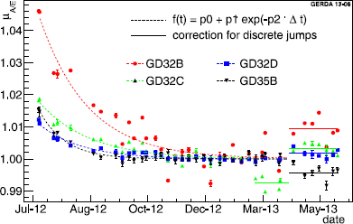
Gaussian mean μ A/E for DEP events for individual 228Th calibrations. The data points in the period before the occurrence of jumps are fitted with an exponential function as specified. Each A/E distribution is normalized such that the constant of the fit (p0) is one. Separate constant corrections are determined as averages over the periods corresponding to the discrete jumps
-
2.
μ A/E increases by up to 1 % during calibration runs which last typically one hour (Fig. 6). During physics data taking, μ A/E returns to the value from before the calibration on a time scale of less than 24 hours, which is short compared to the one week interval between calibrations. This causes μ A/E in calibrations to be shifted to slightly higher values compared to physics data taking. This effect is largely removed by applying a linear correction in time (fit shown in Fig. 6) to calibration data. Afterwards, μ A/E of physics data in the interval 1.0–1.3 MeV agrees approximately with Compton events from calibration data in the same energy region (see Fig. 7).
Fig. 6 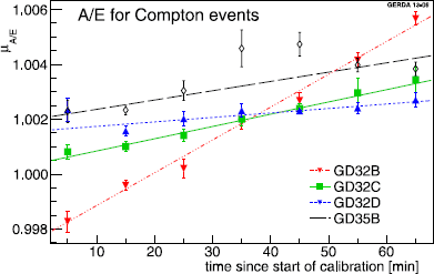
Gaussian mean μ A/E of the A/E distribution for Compton events as a function of the time since the start of a calibration run. The data from all calibrations are combined after the correction according to Fig. 5 has been applied
Fig. 7 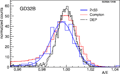
A/E distribution of GD32B from physics data events between 1.0 and 1.3 MeV (blue, dominantly 2νββ decays), Compton continuum in the same energy range (red) and DEP events (black). The latter two are taken from the sum of all calibrations. All corrections are applied. The tail on the left side of the Gaussian is larger in the Compton events due to a higher fraction of MSE compared to the physics data in this energy range (Color figure online)
-
3.
A/E shows a small energy dependence (Fig. 8). It is measured by determining the Gaussian mean μ A/E at different energies in the 208Tl Compton continuum between 600 and 2300 keV. The size is about 0.5 to 1 % per MeV. This approach is documented and validated in Refs. [16, 24]. The correction is applied to both calibration and physics data.
Fig. 8 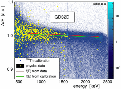
A/E energy dependence shown with 228Th calibration data (blue density plot) and events from physics data taking (predominantly 2νββ, yellow points). The distributions of μ A/E for the different energy bins are fitted with a linear function (green line). The 2νββ continuum is fitted with the same function, leaving only the constant of the fit free (red line). The data from GD32D are shown (Color figure online)


The corrections discussed above are empirical and result in energy and time independent A/E distributions. The origin of the time drifts might be due to electric charges collected from LAr on the surface of the insulating groove. This is a known phenomenon [25] and pulse shape simulations show that A/E changes of the observed size are conceivable. The small observed energy dependence of A/E (item 3) is thought to be an artefact of data acquisition and/or signal processing.
Since A/E has arbitrary units, it is convenient to rescale the distribution at the end such that the mean of the Gaussian is unity after all corrections. This eases the combination of all detectors.
The compatibility of calibration data with physics data after the application of all corrections is verified in Fig. 7. The A/E Gaussian parameters are quantitatively compared in Table 1. The agreement of μ A/E for DEP and 2νββ events validates also the energy dependence correction (item 3). Small differences remain due to imperfections of the applied corrections. They will be taken into account as a systematic uncertainty in the determination of the 0νββ efficiency in Sect. 3.3.
In contrast to the SSE Gaussian, the MSE part of the A/E distribution and the part from p+ electrode events is only negligibly affected by the A/E resolution and its change with energy. This motivates the use of an A/E cut that is constant at all energies: If the cut position is many σ A/E of the Gaussian resolution away from one, the survival fraction is practically independent of the energy. Only at low energies this is no longer the case. At about 1 MeV, the cut position A/E>0.965 corresponds to a separation from one by 2.6 σ A/E corresponding to the 99 % quantile of a Gaussian (see Fig. 9). For lower energies the efficiency loss of the Gaussian peak becomes relevant. Therefore the efficiency determination is restricted to energies above 1 MeV.

Width σ A/E of the A/E Gaussian versus energy (points with error bars) for GD35B with a fit (black dashed line). The blue full line shows the 99 % quantile of the Gaussian (2.6 σ A/E ). The red horizontal line corresponds to the low side PSD cut distance from the nominal μ A/E =1. The uncertainty band is given by the maximal deviation of the A/E scale as determined in Table 1 (Color figure online)
The energy dependence of μ A/E is determined between 600 keV and 2300 keV. Since the dependence is weak, even beyond these limits the cut determination is accurate to within a few percent. This is acceptable for example to determine the fraction of α events at the p+ electrode passing the SSE selection cut.
3.2 Application of PSD to data
Figure 10 shows A/E plotted versus energy for physics data in a wide energy range together with the acceptance range. The data of all detectors have been added after all applicable corrections and the normalization of the Gaussian mean to one. The cut rejects events with A/E<0.965 (“low A/E cut”) or A/E>1.07 (“high A/E cut”). The high side cut interval was chosen twice wider due to the much lower occurrence and better separation of p+ electrode events. The cut levels result in a high probability to observe no background event in the final Q ββ analysis window for the Phase I BEGe data set, while maintaining a large efficiency with small uncertainties. As can be seen from Fig. 9, at Q ββ the cut is ≥4.5 σ A/E apart from one.

A/E versus energy in a wide energy range for the combined BEGe data set. The acceptance region boundaries are marked by the red lines. The blinded region is indicated by the green band (Color figure online)
Figure 11 shows the combined energy spectrum of the BEGe detectors before and after the PSD cut. In the physics data set with 2.4 kg yr exposure, seven out of 40 events in the 400 keV wide region around Q ββ (excluding an 8 keV blinding window) are kept and hence the background for BEGe detectors is reduced from (0.042 ± 0.007) to (\(0.007_{-0.002}^{+0.004}\)) cts/(keV kg yr). In the smaller 230 keV region three out of 23 events remain. Table 2 shows the surviving fractions for several interesting energy regions in the physics data and 228Th calibration data. The suppression of the 42K γ line at 1525 keV in physics data is consistent with the one of the 212Bi line at 1621 keV. The rejection of α events at the p+ electrode is consistent with measurements with an α source in a dedicated setup [17].

Energy spectrum of the combined BEGe data set: grey (blue) before (after) the PSD cut. The inset shows a zoom at the region Q ββ ±200 keV with the 8 keV blinded region in green (Color figure online)
The energy spectrum of the physics data can be used to identify the background components at Q ββ as described in Ref. [1]. About half of the events are from 42K decays on the n+ electrode surface which are rejected by the low side A/E cut with large efficiency [19]. About one third of the background at Q ββ is due to 214Bi and 208Tl. Their survival probability can be determined from the calibration data (52 % for 208Tl) or extrapolated from previous studies [21, 22] (36 % for 214Bi). The remaining backgrounds e.g. from 68Ga inside the detectors and from the p+ surface are suppressed efficiently [15, 17]. The rejection of 80 % of the physics events at Q ββ is hence consistent with expectation.
In Fig. 12, the A/E distribution of physics data in the Q ββ ±200 keV region is compared with the distributions from different background sources. The peak at 0.94 can be attributed to n+ surface events. The A/E distribution of the other events is compatible within statistical uncertainty with the ones expected from the different background sources.

A/E histogram of the physics data within 200 keV of Q ββ (red) compared to Compton continuum events (green dot-dot-dashed) and 1621 keV FEP events (black) from calibration data. Also shown are simulations of 42K decays at the n+ electrode surface (blue dashed) and 60Co (black dot-dashed) [15]. The scalings of the histograms are arbitrary. Three physics data events have large A/E values (p+ electrode events) and are out of scale. The accepted interval is shown in grey (Color figure online)
3.3 Evaluation of 0νββ cut survival fraction for BEGes
The PSD survival fraction of DEP events can vary from the one for 0νββ events because of the difference of the event locations in a detector (see Sect. 2.3) and due to the different energy release and the resulting bremsstrahlung emission.
The influence of these effects was studied by simulations. The first effect was irrelevant in past publications since only a low A/E cut was studied and p+ electrode events have higher A/E. In the present analysis, we required also A/E<1.07. Therefore we use a pulse shape simulation of 0νββ events [15] to determine the rejected fraction of signal events by the high A/E cut.
The second effect can influence the low A/E cut survival. To estimate its size, we compare the pulse shape simulation result [15] with a Monte Carlo simulation [16] which selects events according to the bremsstrahlung energy. The latter is approximately equivalent to a cut on the spatial extent of the interaction since higher energy bremsstrahlung γ rays interact farther from the main interaction site (electron-positron pair creation vertex for DEP or 0νββ decay vertex). The fraction of DEP events with a Compton scattering before the pair creation was taken into account. The determined fraction of MSE in DEP and 0νββ events was the same within uncertainties. In contrast, the pulse shape simulation removes 1.8 % events more for A/E<0.965. This difference could be caused by a larger fraction of bremsstrahlung in 0νββ compared to DEP or due to simulation artefacts [15]. Here we follow the result of the Monte Carlo simulation, i.e. use the DEP survival fraction for the low A/E cut, and take the difference to the pulse shape simulation as systematic error.
Thus, the survival fraction ϵ 0νββ of the 0νββ signal is estimated as follows:
-
the rejected fraction for the low side cut of 0.054 is determined from DEP events (Table 2). This value varies from 0.042 ± 0.006 to 0.062 ± 0.010 for the different detectors and is hence within uncertainties the same for all of them.
-
the rejected fraction by the high A/E cut of 0.025 is determined from the 0νββ pulse-shape simulation [15].
Finally, the efficiency is ϵ 0νββ =0.92±0.02. The uncertainty is the quadratic sum of the following components:
-
statistical uncertainty of the DEP survival fraction: 0.003
-
uncertainty from the A/E energy dependence (item 3 in Sect. 3.1): 7.5×10⁻⁵
-
uncertainty due to the residual differences between calibration and physics data (change of the cut by the largest difference between μ A/E for 2νββ and Compton events in Table 1): 0.004
-
systematic uncertainty due to the difference between the survival fraction of 0νββ from the pulse shape simulation [15] and the one measured with DEP events: 0.018.
The 0νββ survival fraction can be cross checked with the one determined for 2νββ decays. The energy region is chosen between 1 and 1.45 MeV to exclude the γ lines at 1461 keV from 40K and 1525 keV from 42K. The spectral decomposition of the BEGe data [1] yields a fraction of f 2νββ =0.66±0.03 of 2νββ decays. The parts f i of the remaining components are listed in Table 3 together with the PSD survival fractions ϵ i . The background origins mostly from Compton scattered γ quanta. The fractions ϵ i were extrapolated from several studies involving experimental measurements as well as simulations. For 228Th, ϵ i is determined from present calibration data.
The PSD survival fraction for 2νββ decays ϵ 2νββ is then related to the overall PSD survival fraction for events in the interval ϵ data=0.748 ±0.011 (Table 2) by:
The resulting survival fraction of 2νββ events is ϵ 2νββ =0.90±0.05. This number needs a small correction due to decays in the n+ transition layer. The long pulse rise time for these events (see Sect. 2.1) leads to a ballistic deficit in the reconstructed energy, i.e. 0νββ events do not reconstruct at the peak position. This loss is already accounted for in the definition of the dead layer thickness. For 2νββ events the energy spectrum is continuous, i.e. the effective dead volume is smaller. But A/E is reduced as well and a fraction of about 0.015 ± 0.005 is rejected according to simulations. For the comparison with the 0νββ PSD survival fraction, this correction should be added such that finally a fraction of 0.91 ± 0.05 is obtained. It agrees well with ϵ 0νββ = 0.92 ± 0.02.
3.4 PSD summary for BEGe detectors
Due to their small area p+ contact BEGe detectors offer a powerful pulse shape discrimination between 76Ge 0νββ signal events of localized energy deposition and background events from multiple interactions in the detector or energy deposition on the surface.
The parameter A/E constitutes a simple discrimination variable with a clear physical interpretation allowing a robust PSD analysis. The characteristics of this quantity have been studied for several years and are applied for the first time in a 0νββ analysis. 228Th data taken once per week are used to calibrate the performance of A/E and to correct for the observed time drifts and small energy dependencies. The whole procedure of the PSD analysis was verified using 2νββ events from 76Ge recorded during physics data taking.
The chosen cut accepts a fraction of 0.92 ± 0.02 of 0νββ events and rejects 33 out of 40 events in a 400 keV wide region around Q ββ (excluding the central 8 keV blinded window). The latter is compatible with the expectation given our background composition and PSD rejection. The background index is reduced to (\(0.007_{-0.002}^{+0.004}\)) cts/(keV kg yr).
Applying the PSD cut to 2νββ events results in an estimated 0νββ signal survival fraction of 0.91 ± 0.05 that agrees very well with the value extracted from DEP and simulations.
4 Pulse shape discrimination for semi-coaxial detectors
In the current Phase I analysis, three independent pulse shape selections have been performed for the semi-coaxial detectors. They use very different techniques but it turns out that they identify a very similar set of events as background. The neural network analysis will be used for the 0νββ analysis while the other two (likelihood classification and PSD selection based on the pulse asymmetry) serve as cross checks.
All methods optimize the event selection for every detector individually. They divide the data into different periods according to the noise performance. Two detectors (ANG 1 and RG 3) had high leakage current soon after the deployment. The analyses discussed here consider therefore only the other six coaxial detectors.
4.1 Pulse shape selection with a neural network
The entire current pulse or—to be more precise—the rising part of the charge pulse is used in the neural network analysis. The following steps are performed to calculate the input parameters:
-
baseline subtraction using the recorded pulse information in the 80 μs before the trigger. If there is a slope in the baseline due to pile up, the event is rejected. This selection effects practically only calibration data,
-
smoothing of the pulse with a moving window averaging of 80 ns integration time,
-
normalization of the maximum pulse height to one to remove the energy dependence,
-
determination of the times when the pulse reaches 1,3,5,…,99 % of the full height. The time when the pulse height reaches A 1=50 % serves as reference. Due to the 100 MHz sampling frequency, a (linear) interpolation is required between two time bins to determine the corresponding time points (see Fig. 13).
Fig. 13 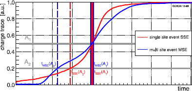
Example physics data pulses for SSE and MSE candidate events. The determination of the input parameters for the TMVA algorithms is shown for pulse heights A 1 and A 2

The resulting 50 timing informations of each charge pulse are used as input to an artificial neutral network analyses. The TMVA toolkit implemented in ROOT [26] offers an interface for easy processing and evaluation. The selected algorithm TMlpANN [27] is based on multilayer perceptrons. Two hidden layers with 51 and 50 neurons are used. The method is based on the so called “supervised learning” algorithm.
Calibration data are used for training. DEP events in the interval 1593 keV ±1⋅FWHM serve as proxy for SSE while events of the full energy line of 212Bi in the equivalent interval around 1621 keV are dominantly MSE and are taken as background sample. Figure 14 shows as an example of the separation power the distribution of the time of 5 % and 81 % pulse height for the two event classes. Note that both event classes are not pure samples but a mixture of SSE and MSE because of the Compton events under the peaks.

Time distribution for crossing the 5 % (left) and 81 % (right) pulse height for 228Th calibration events with energy close to the DEP (red) and close to the 1621 keV FEP (blue) (Color figure online)
The calibrations are grouped in three intervals. The first period spans from the start of data taking to July 2012 when the detector configuration and some electronics was changed (p1). The second period (p2) lasts the first four weeks afterwards and the third period (p3) the rest of Phase I. For RG 2, the second period spans until November 2012 when its operating voltage was reduced. For each period at least 5000 events are available per detector and event class for training.
The output of the neural network is a qualifier, i.e. a number between ≈0 (background like event) and ≈1 (signal like event). Figure 15 shows a scatter plot of this variable versus the energy. The distribution peaks for DEP events at higher qualifier values while for FEP events at 1621 keV and SEP events at 2104 keV the intensity is shifted to lower values. The qualifier distribution from Compton events at different energies can be compared to estimate a possible energy dependence of the selection (see Fig. 16). For most detectors no drift is visible. Only RG 2 shows a larger variation. An energy dependent empirical correction of the qualifier is deduced from such distributions.

TMlpANN response versus energy for 228Th calibration events. Shown is the distribution for RG 1. The line at ∼0.38 marks the position for 90 % DEP survival fraction

TMlpANN response for Compton events for RG 2 at different energies. The energy dependence for RG 2 is about twice bigger than for any other detector
The qualifier threshold which keeps 90 % of the DEP events is determined for each detector and each period individually. The cut values vary between 0.31 and 0.42. Figure 17 shows a 228Th calibration spectrum with and without PSD selection. For the analysis, the survival fraction of MSE is studied. The survival is defined as the fraction of the peak content remaining after the cut, i.e. the Compton events under the peak are subtracted by scaling linearly the event counts from energies below and above the peak. The fractions are listed in Table 4 for the different periods. The last column lists the number of events in the 230 keV window around Q ββ before and after the cut. About 45 % of the events are classified as background.

228Th calibration spectrum without and with TMlpANN pulse shape discrimination for ANG 3. The PSD cut is fixed to retain 90 % of DEP events (see inset)
Figure 18 shows the ANN response for DEP and SEP events. Shown are also the qualifier distributions for different samples from physics data taking: from the interval 1.0–1.4 MeV (dominantly 2νββ events, MSE part subtracted), from the 1525 keV 42K γ line (dominantly MSE) and the qualifier for events in the 230 keV window. The events from the 1525 keV gamma peak are predominantly MSE and the shape agrees with the SEP distribution. The events in the 1.0–1.4 MeV region are dominantly SSE and their distribution agrees quite well with the one for DEP events. The red curve shows the DEP survival fraction versus the cut position (right scale).

ANN response for 228Th calibration events for DEP (green, long dashes) and SEP (dark blue) for ANG 3 in the first period. The distributions from Compton events at these energies are subtracted statistically using events in energy side bands. Also shown in black are the qualifier values of events from physics data taking from a 230 keV window around Q ββ . The grey vertical line marks the cut position. Physics data events from the 1525 keV FEP of 42K are shown in magenta and the ones from the interval 1.0–1.4 MeV by brown dashes (dominantly 2νββ, MSE part subtracted) (Color figure online)
The training was performed for the periods individually by combining all calibration data. The rules can then be applied to every single calibration to look for drifts in time. Figure 19 shows the DEP survival fraction (blue triangles) for the entire Phase I from November 2011 to May 2013 for all detectors. The plots show a stable performance. Also shown are the equivalent entries (red circles) for events with energy around the SEP position. For several detectors the rejection of MSE is not stable. Especially visible is the deterioration starting in July 2012. This is related to different conditions of high frequency noise.

DEP (blue) and SEP (red) survival fraction for individual calibrations for the entire Phase I (Color figure online)
The distribution of the qualifier for all events in the 230 keV window around Q ββ is shown in Fig. 20. Events rejected by the neural network are marked in red. Circles mark events rejected by the likelihood method and diamonds those rejected by the method based on the current pulse asymmetry. Both methods are discussed below. In the shown energy interval, all events removed by the neural network are also removed by at least one other method and for about 90 % of the cases, all three methods discard the events. In a larger energy range about 3 % of the rejected events are only identified by the neural network.

Neural network qualifier for events with energy close to Q ββ . Events marked by a red dot are rejected. Circles and diamonds mark events which are rejected by the likelihood analysis and the method based on the pulse asymmetry, respectively (Color figure online)
Figure 21 shows the energy spectrum of all semi-coaxial detectors added up before and after the PSD selection.

Energy spectrum of semi-coaxial detectors with and without neural network PSD selection
4.2 Systematic uncertainty of the neural network signal efficiency
In this analysis we use the survival fraction of DEP events as efficiency for 0νββ events.
The distribution of DEP events in a detector is not homogeneous since the probability for the two 511 keV photons to escape is larger in the corners. It is therefore conceivable that the ANN—instead of selecting SSE—is mainly finding events at the outer surface. The DEP survival fraction would in this case not represent the efficiency for 0νββ decay which are distributed homogeneously in the detector.
2νββ events are also SSE and homogeneously distributed inside the detector. Hence a comparison of its pulse shape identification efficiency with the preset 0.90 value for DEP events is a powerful test.
Another SSE rich sample are events at the Compton edge of the 2614.5 keV γ line. The energy range considered is 2.3–2.4 MeV, i.e. higher than Q ββ . The comparison to the DEP survival fraction allows also to check for an energy dependence. The distribution of Compton edge events in detector volume is similar to DEP.
4.2.1 Efficiency of 2νββ for neural network PSD
The energy range between 1.0 and 1.3 MeV (position of the Compton edge of the 1525 keV line) is suited for the comparison of the SSE efficiency. At lower energies the electronic noise will deteriorate the discrimination between SSE and MSE. In this interval, the data set consists to a fraction f 2νββ =0.76±0.01 of 2νββ decays according to the Gerda background model [1]. The remaining 24 % are Compton events predominantly of the 1525 keV line from 42K decays, of the 1460 keV line from 40K decays and from 214Bi decays. Hence it is a good approximation to use the pulse shape survival fraction ϵ Compton from the calibration data to estimate the suppression of the events not coming from 2νββ decays. Typical values for ϵ Compton are between 0.6 and 0.7 for the different detectors, i.e. higher than the values quoted in Table 4 due to a small energy dependence (see Fig. 17).
Figure 22 shows the physics data (red) overlayed with the background model (blue, taken from Ref. [1]) and the same distributions after the PSD cut (in magenta for the data and in light blue for the model). For the model, the 2νββ fraction is scaled by the DEP survival rate while the remaining fraction is scaled according to ϵ Compton taken from the 228Th calibration data for each detector. Both pairs of histograms agree roughly in the range 1.0–1.3 MeV. This is qualitatively confirmed if the 2νββ PSD efficiency is calculated using (2). Its distribution is also shown as the green filled histogram in Fig. 22. The average efficiency for the range 1.0–1.3 MeV is ϵ 2νββ =0.85±0.02 where the error is dominated by the systematic uncertainty of ϵ Compton. The latter is estimated by a variation of the central value by 10 % which is the typical variation of ϵ Compton between 1 MeV and 2 MeV.

Effect of the PSD selection on the data (in red and magenta) and the expected effect on the background model (dark blue dotted and light blue dashed). Overlayed is also the extracted PSD efficiency (green filled histogram) for 2νββ events (right side scale) (Color figure online)
The obtained efficiency ϵ 2νββ is close to the DEP survival fraction of ϵ DEP=0.9 and indicates that there are no sizable systematic effects related to the differences in the distribution of DEP and 2νββ events in the detectors.
4.2.2 Neural network PSD survival fraction of Compton edge events
Calibration events at the Compton edge of the 2615 keV γ line, i.e. in the region close to 2.38 MeV, are enhanced in SSE and distributed similar to DEP events in the detector. The qualifier distribution for these events can be approximated as a linear combination of the DEP distribution and the one from multiple Compton scattered γ ray events (MCS). Events with energy larger than the Compton edge (e.g. in the interval 2420–2460 keV) consists almost exclusively of MCS. The total counts in the qualifier interval 0 to 0.2 for Compton edge events and MCS are used for normalization and the MCS distribution is then subtracted.
The “MCS subtracted” Compton edge distribution (red curve in Fig. 23) shows an acceptable agreement with the DEP distribution (green dotted curve). The survival fraction is defined as the part above the selection cut. Its value varies for the 3 periods and the 6 detectors between 0.85 and 0.94. No systematic shift relative to the DEP value e.g. due to an energy dependence of the efficiency is visible. If SEP events are used to model the multi site event contribution, consistent values are obtained.

Qualifier distribution for events at the Compton edge (magenta) as a linear combination of MCS (blue) and DEP (green dotted) distributions. The Compton edge distribution after the subtraction of the SEP part is shown in red (Color figure online)
4.2.3 Summary of systematic uncertainties
The cross checks of the PSD efficiency address a possible energy dependence and a volume effect due to the different distributions of DEP and 0νββ events. All studies performed are based on calibration or physics data and are hence independent of simulations.
The possible deviations from 0.90 seen are combined quadratically and scaled up to allow for additional sources of systematic uncertainties. The 0νββ efficiency is \(\epsilon_{\mathit {ANN}}=0.90^{+0.05}_{-0.09}\).
4.3 Alternative PSD methods
Two more PSD methods have been developed. They are used here to cross check the event selection of the neural network method (see Fig. 20). No systematic errors for the signal efficiency has been evaluated for them.
4.3.1 Likelihood analysis
In a second PSD analysis, 8 input variables calculated from the charge pulse trace are used as input to the projective likelihood method implemented in TMVA. Each input variable is the sum of four consecutive pulse heights of 10 ns spacing after baseline subtraction and normalization by the energy. The considered trace is centered around the time position where the derivative of the original trace is maximal, i.e. around the maximum of the current.
The training is performed for two periods: before (pI) and after (pII) June 2012. Instead of DEP events, the Compton edge in the interval 2350–2370 keV is used as signal region and the interval 2450–2570 keV as background sample. The latter contains only multiple Compton scattered photons and is hence almost pure MSE. The Compton edge events are a mixture of SSE and MSE. From the two samples a likelihood function for signal L sig and background L bkg like events is calculated and the qualifier q PL is the ratio q PL=L sig/(L sig+L bkg).
Figure 24 shows for the calibration data the scatter plot of the qualifier versus energy. The separation of DEP (1593 keV) and FEP at 1621 keV is visible by the different population densities at low and high qualifier values. The cut position is independent of energy and fixed to about 0.80 survival fraction for DEP events. The SEP survival fractions and for comparison also the ones for several other subsets are listed in Table 5. About 65 % of the events in the 230 keV window around Q ββ are rejected.

Likelihood response versus energy distribution for 228Th calibration events. Data are shown for ANG 3
Figure 25 shows the distribution of the qualifier for different event classes. The distribution for physics data events from the 42K line are well described by the FEP distribution in calibration data and the events in the 1.0–1.4 MeV interval are clearly enhanced in SSE as expected for 2νββ events.

Likelihood response for 228Th calibration DEP (green dotted) and FEP (dark blue dashed) events for ANG 3. The distributions from Compton events at these energies are subtracted statistically using events in energy side bands. Also shown in black are the qualifier values of events from physics data taking from a 230 keV window around Q ββ . The grey vertical line marks the cut position. Shown are also distributions of physics data events from the 42K γ line (light blue) and from the interval 1.0–1.4 MeV (red, dominantly 2νββ) (Color figure online)
4.3.2 PSD based on pulse asymmetry
In a third approach, only two variables are used to select single site events for the semi-coaxial detectors. As discussed above, the A/E variable alone is not a good parameter for semi-coaxial detectors. However, if A/E is combined with the pulse asymmetry, the PSD selection is much more effective. The asymmetry A s is defined as
Here I(i) is the current pulse height, i.e. the differentiated charge pulse at time i, and n m the time position of the maximum. A window of 200 samples (i.e. a 2 μs time interval) around the time of the trigger is analyzed.
To reduce noise, different moving window averaging with integration times of 0 (no filter), 20, 40, 80, 160 and 320 ns for the charge pulse are applied. For each shaping time, A/E and A s are determined. Empirically, the combination
exhibits good PSD performance. For SSE, the current pulse might contain more than one maximum (Fig. 3). To reduce ambiguities, A S is shaped with larger integration times.
An optimization is performed by comparing the DEP survival fraction ϵ DEP from calibration data to the fraction of background events f bkg between 1700 and 2200 keV (without a 40 keV blinded interval around Q ββ ) that remains after the PSD selection. The lower cut value of the qualifier q AS is determined by maximizing the quantity \(S=\epsilon_{\mathrm{DEP}} / \sqrt{f_{\mathrm{bkg}} + 3/N_{\mathrm{bkg}}}\); the upper cut is fixed at ≈+4σ of the Gaussian width of the DEP qualifier distribution (see Fig. 26). All combinations of shaping times for A/E and A s are scanned as well as different values for c in the range of 1–4. The one with the highest S is selected.

Distribution of qualifier for DEP (dotted green) and FEP (dashed dark blue) calibration events for ANG 3 after a statistical subtraction of the Compton events below the peaks. The grey band marks the acceptance range. Overlayed are also the PSD qualifier for physics data in the 230 keV window around Q ββ (black), data events from the 1525 keV 42K peak (light blue) and from the interval 1.0–1.4 MeV (dark green dotted). The DEP survival fraction is displayed in red (right scale) (Color figure online)
The term 3/N bkg with N bkg being the total number of background events is added to avoid an optimization for zero background. For N bkg≈40 the optimization yields a DEP survival fraction of 0.7–0.9 (see Table 6) and about 75 % of the events in the interval 1.7–2.2 MeV are rejected.
Figure 27 shows a scatter plot of the PSD qualifier versus the energy. A separation between the DEP and multi site events at the energy of the FEP or SEP is visible. Figure 26 shows qualifier distributions for DEP and FEP calibration events after Compton events below the peaks are statistically subtracted. Overlayed is also the PSD qualifier for physics data in the 230 keV window around Q ββ (black histogram), from the 1525 keV γ line (light blue) and the interval 1.0–1.4 MeV (yellow). The right scale shows the DEP survival fraction (red) as a function of the cut position. The grey area indicates the accepted range. The qualifier distribution of physics data around Q ββ has a larger spread than the one of FEP events. This is the reason why events at Q ββ are rejected stronger than MSE (see Table 6). A possible explanation is that the physics data contain a large fraction of events which are not MSE. These can be for example surface p+ events. The “maximal” background model of Gerda [1] is compatible with a significant fraction of p+ events. A pulse shape simulation also shows that the selection corresponds to a volume cut: events close to the p+ contact and in the center of the detectors are removed.

Distribution of the ANG 3 qualifier versus energy for 228Th calibration data for the PSD based on the pulse asymmetry
4.4 Summary of PSD analysis for coaxial detectors
For the semi-coaxial detectors three different PSD methods are presented following quite different concepts. The one based on an artificial neural network will be used for the 0νββ analysis. It has been tuned to yield 90 % survival fraction for DEP events of the 2.6 MeV γ line of 208Tl decays. Most of these events are SSE like 0νββ decays. For the study of a possible volume effect and energy dependence of the efficiency, 2νββ decays (ϵ 2νββ =0.85±0.02) and events with energy close the Compton edge (efficiency between 0.85 and 0.95) have been used. We conclude that the 0νββ efficiency is \(\epsilon_{\mathrm{ANN}} = 0.90^{+0.05}_{-0.09}\).
The event selection of the neural network is cross checked by two other methods. One is based on a likelihood ratio. Training is performed with events at the Compton edge (SSE rich) and at slightly higher energies (almost pure MSE). For a cut with a DEP survival fraction of about 0.8 only 45 % of the events around Q ββ remain.
Another method is only based on the A/E parameter and the current pulse asymmetry A S . Different signal shapings are tried and an optimization of a signal over background ratio is performed. The DEP survival fraction varies between 0.7 and 0.9 for the different detectors and periods. The background is reduced by a factor of four.
Of the events rejected by the neural network analysis in the 230 keV window around Q ββ , about 90 % are also identified as background by both other methods. This gives confidence that the classification is meaningful.
5 Summary
The neural network analysis rejects about 45 % of the events around Q ββ for the semi-coaxial detectors and the A/E selection reduces the corresponding number for BEGe detectors by about 80 %. With a small loss in efficiency the Gerda background index is hence reduced from (0.021±0.002) cts/(keV kg yr) to (0.010±0.001) cts/(keV kg yr). These values are the averages over all data except for the period p2, the “silver” data set, that covers the time period around the BEGe deployment and which corresponds to 6 % of the Phase I exposure [1].
The estimated 0νββ decay signal efficiencies for semi-coaxial detectors are \(0.90^{+0.05}_{-0.09}\) and for BEGe detectors 0.92±0.02. Despite this loss of efficiency, the Gerda sensitivity defined as the expected median half life limit of the 0νββ decay improves by about 10 % with the application of the pulse shape discrimination.
References
M. Agostini et al. (Gerda Collaboration), arXiv:1306.5084. Eur. Phys. J. C (submitted)
K.H. Ackermann et al., Eur. Phys. J. C 73, 2330 (2013)
F.S. Goulding et al., IEEE Trans. Nucl. Sci. NS-31, 285 (1984)
J. Roth et al., IEEE Trans. Nucl. Sci. NS-31, 367 (1984)
D. Gonzalez et al., Nucl. Instrum. Methods Phys. Res., Sect. A 515, 634 (2003)
F. Petry et al., Nucl. Instrum. Methods Phys. Res., Sect. A 332, 107 (1993)
B. Majorovits, H.V. Klapdor-Kleingrothaus, Eur. Phys. J. A 6, 463 (1999)
J. Hellmig, H.V. Klapdor-Kleingrothaus, Nucl. Instrum. Methods Phys. Res., Sect. A 455, 638 (2000)
H.V. Klapdor-Kleingrothaus et al., (HdM Collaboration), Eur. Phys. J. A 12, 147 (2001)
C.E. Aalseth et al., (Igex Collaboration) Phys. Rev. D 65, 092007 (2002)
Canberra Semiconductor NV, Lammerdries 25, B-2439 Olen, Belgium
M. Agostini et al., J. Instrum. 6, P08013 (2011)
M. Agostini et al., J. Phys. Conf. Ser. 368, 012047 (2012)
Z. He, Nucl. Instrum. Methods Phys. Res., Sect. A 463, 250 (2001)
M. Agostini et al., J. Instrum. 6, P03005 (2011). arXiv:1012.4300
D. Budjáš et al., J. Instrum. 4, P10007 (2009). arXiv:0909.4044
M. Agostini, Dissertation, Technical University Munich, 2013
E. Aguayo et al., Nucl. Instrum. Methods Phys. Res., Sect. A 701, 176 (2013). arXiv:1207.6716
A. Lazzaro, Master’s thesis, University Milan Bicocca, 2012
M. Barnabé Heider et al., J. Instrum. 5, P10007 (2010)
M. Agostini et al., J. Phys. Conf. Ser. 375, 042009 (2012)
M. Heisel, Dissertation, University of Heidelberg, 2011
P. Medina, C. Santos, D. Villaume, in Procs. of the 21st IEEE (IMTC 04), vol. 3 (2004), p. 1828
D. Budjáš, Dissertation, University of Heidelberg, 2009
M. Barnabé Heider et al., arXiv:0812.1907
Acknowledgements
The Gerda experiment is supported financially by the German Federal Ministry for Education and Research (BMBF), the German Research Foundation (DFG) via the Excellence Cluster Universe, the Italian Istituto Nazionale di Fisica Nucleare (INFN), the Max Planck Society (MPG), the Polish National Science Centre (NCN), the Foundation for Polish Science (MPD programme), the Russian Foundation for Basic Research (RFBR), and the Swiss National Science Foundation (SNF). The institutions acknowledge also internal financial support.
The Gerda Collaboration thanks the directors and the staff of the LNGS for their continuous strong support of the Gerda experiment.
We acknowledge guidance concerning the n+ surface layer modeling from D. Radford.
Open Access
This article is distributed under the terms of the Creative Commons Attribution License which permits any use, distribution, and reproduction in any medium, provided the original author(s) and the source are credited.
Author information
Authors and Affiliations
Corresponding author
Rights and permissions
Open Access This article is distributed under the terms of the Creative Commons Attribution 2.0 International License (https://creativecommons.org/licenses/by/2.0), which permits unrestricted use, distribution, and reproduction in any medium, provided the original work is properly cited.
About this article
Cite this article
Agostini, M., Allardt, M., Andreotti, E. et al. Pulse shape discrimination for Gerda Phase I data. Eur. Phys. J. C 73, 2583 (2013). https://doi.org/10.1140/epjc/s10052-013-2583-7
Received:
Published:
DOI: https://doi.org/10.1140/epjc/s10052-013-2583-7