
Abstract
The detrended fluctuation analysis (DFA) and its variants are popular methods to analyze the self-similarity of a signal. Two steps characterize them: firstly, the trend of the centered integrated signal is estimated and removed. Secondly, the properties of the so-called fluctuation function which is an approximation of the standard deviation of the resulting process is analyzed. However, it appears that the statistical mean was assumed to be equal to zero to obtain it. As there is no guarantee that this assumption is true a priori, this hypothesis is debatable. The purpose of this paper is to propose two alternative definitions of the fluctuation function. Then, we compare all of them based on a matrix formulation and the filter-based interpretation we recently proposed. This analysis will be useful to show that the approach proposed in the original paper remains a good compromise in terms of accuracy and computational cost.
Graphic abstract


Data availability statement
This manuscript has no associated data or the data will not be deposited. [Authors’ comment: The synthetic data can be computed thanks to the Matlab Toolbox FracLab available at the following https://project.inria.fr/ fraclab/.]
Notes
Weierstrass (WEI) functions are continuous functions that can be derived from nowhere [6]. Each WEI is constructed as a sum of damped sinusoids with increasing frequencies: \(WEI(t)=\sum _{n=1}^{+\infty }\lambda ^{-nH}sin(\lambda ^nt)\) with \(\lambda \ge 2\).
Indeed, if the detrended profile is assumed to be taken at time \(\frac{k}{f_s}\) with \(f_s\) the sampling frequency, the first sequence decimated by a factor N is characterized by the samples taken at time \(\frac{k}{f_s}N\).
To avoid any misunderstanding, it should be noted that these subsequences are not the local trends.
Let X be a random variable. When the statistical mean E[X] is known, an estimation of the variance \(V_X=E\big [X^2\big ]-E^2[X]\) using L values of the random variable \(\{X_i\}_{i=0,...,L-1}\) is \( \hat{V}_{X}=\frac{1}{L}\sum _{i=0}^{L-1}(X_i-E[X])^2\). In practice, the statistical mean being unknown is replaced by its estimate \(X_{mean} =\frac{1}{L} \sum _{i=0}^{L-1}X_{i}\). Therefore the empirical variance is \( \hat{V}_{X}=\frac{1}{L}\sum _{i=0}^{L-1}(X_i-X_{mean})^2=\frac{1}{L}\sum _{i=0}^{L-1} X_i^2-X_{mean}^2\). As \(E[X_{mean}^2]=\frac{1}{L}E[X^2]+\frac{L-1}{L}E^2[X]\), this estimator has the following mean and variance:
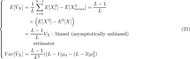
where \(\mu _k\) is the \(k^{th}\) central moment of X. In the Gaussian case, \(\mu _{2p+1}=0\) and \(\mu _{2p} =\frac{2p!}{2^p p!} V_X^p\). Therefore, \(Var[\hat{V}_{X}]=\frac{2(L-1)}{L^2}V_X^2\). When this estimator is averaged over N realizations, its variance has the advantage of being divided by N.
An alternative unbiased estimator \(\tilde{V}_{X}=\frac{L}{L-1}\hat{V}_{X}\) could be considered. It can be shown that its variance is \( Var[\tilde{V}_{X}]=\frac{1}{L}(\mu _4-\frac{L-3}{L-1}\mu _2^2)\). In the Gaussian case, \(Var[\tilde{V}_{X}(L)]=\frac{2}{L-1}V_X^2\). The variance of this estimator is larger than the variance of \(\hat{V}_{X}\).
When the mean is assumed to be zero, \(J_L\) reduces to \(I_L\) and \(\sum _{n=1}^N(D_n^TJ_L^TJ_LD_n)=\sum _{n=1}^N (D_n^TD_n)=I_{LN}\).
When the value is negative, it corresponds to subdiagonals below the main diagonal. When the value is positive, it corresponds to subdiagonals above the main diagonal.
Once again, when the mean is assumed to be zero, \(J_N\) reduces to \(I_N\) and \(\sum _{l=1}^L(E_l^TJ_N^TJ_NE_l) =\sum _{l=1}^L(E_l^TE_l)=I_{LN}\).
This can be done using the free Matlab Toolbox FracLab available at the following url: https://project.inria.fr/fraclab/.
Simulations were conducted from \(H=0.1\) to \(H=0.9\) with a step equal to 0.1. As the same type of comments can be drawn for any value of H, we only provide the results for \(H=0.1\), \(H=0.5\) and \(H=0.9\).
When \(\lambda =0\), the method corresponds to the DFA.

References
J. Gao, H. Jing, F. Liu, Y. Cao, Multiscale entropy analysis of biological signals: A fundamental bi-scaling law. Front. Comput. Neurosci. 9, 1–64 (2015)
F. Zappasodi, E. Olejarczyk, L. Marzetti, G. Assenza, V. Pizzella, F. Tecchio, Fractal dimension of EEG activity senses neuronal impairment in acute stroke. PLoS One 9, 1–8 (2014)
A.K. Mishra, S. Raghav, Local fractal dimension based ECG arrhythmia classification. Biomed. Signal Process. Control 5(2), 114–123 (2010)
D. Kelty-Stephen, J. Anastas, Fractal fluctuations in gaze speed visual search. Atten. Percept. Psychophys. 73, 666–77 (2010)
V. Pitsikalis, P. Maragos, Analysis and classification of speech signals by generalized fractal dimension features. Speech Commun. 51(12), 1206–1223 (2009)
G.H. Hardy, On weierstrass non-differentiable functions. Trans. Am. Math. Soc. 17(3), 301–325 (1916)
A. Benassi, S. Jaffard, D. Roux, Elliptic Gaussian random processes. Rev. Math. Iberoam. 13, 19–90 (1997)
A. Ayache, J. Lévy Véhel, On the identification of the pointwise hölder exponent of the generalized multifractional brownian motion. Stoch. Process. Appl. 111(1), 119–156 (2004)
J. Lévy Véhel, S. Seuret, 2-microlocal Formalism. [Research Report] RR-4741, INRIA, 2003. (inria-00071846)
P. Legrand, “Débruitage et interpolation par analyse de la régularité hölderienne : application à la modélisation du frottement pneumatique-chaussée,” PhD, Doctoranl school Univ. Nantes, with École centrale de Nantes (In French) , Supervisor: J. Lévy Véhel, et M.-T. Do, (2011)
C.K. Peng, S.V. Buldyrev, A.L. Goldberger, S. Havlin, F. Sciortino, M. Simons, H.E. Stanley, Long-range correlations in nucleotide sequences. Nature 356, 168–170 (1992)
R. Sun, “Fractional order signal processing: techniques and applications,” Thesis of Master of science in electrical Engineering, Utah State University (2007)
G. Rilling, P. Flandrin, P. Gonçalves, “Empirical mode decomposition, fractional gaussian noise and hurst exponent estimation,” International Conference on Acoustics, Speech and Signal Processing, pp. 489–492 (2005)
P. Abry, P. Flandrin, M.S. Taqqu, D. Veitch, “Self-similarity and long-range dependence through the wavelet lens,” Theory and Applications of Long-range Dependence, pp. 527–556 (2003)
H.E. Hurst, Long-term storage capacity of reservoirs. Trans. Am. Soc. Civ. Eng. 116, 770–799 (1951)
M.S. Taqqu, V. Teverovsky, W. Willinger, Estimators for long range dependence: An empirical study. Fractals 3(4), 785–788 (1995)
M.S. Taqqu, V. Teverovsky, “On estimating the intensity of long range dependence in finite and infinite variance time series,” A practical guide to heavy tails: statistical techniques and applications, pp. 177–217 (1996)
C.K. Peng, S.V. Buldyrev, S. Havlin, M. Simons, H.E. Stanley, A.L. Goldberger, Mosaic organization of DNA nucleotides. Phys. Rev. E 49(2), 1685–1689 (1994)
M.A. Riley, S. Bonnette, N. Kuznetsov, S. Wallot, J. Gao, A tutorial introduction to adaptive fractal analysis. Front. Physiol. 3, 371 (2012)
B. Berthelot, E. Grivel, P. Legrand, J.-M. André, P. Mazoyer, T. Ferreira, “Filtering-based Analysis Comparing the DFA with the CDFA for Wide Sense Stationary Processes,” In: EUSIPCO 2019 (2019)
B. Berthelot, E. Grivel, P. Legrand, J.-M. André, P. Mazoyer, “Regularized DFA to study the gaze position of an airline pilot,” In: EUSIPCO 2020 (2020)
L. Xu, P.C. Ivanov, K. Hu, Z. Chen, A. Carbone, H.E. Stanley, Quantifying signals with power-law correlations: A comparative study of detrended fluctuation analysis and detrended moving average techniques. Phys. Rev. E 71(5), 051101 (2005)
E. Alessio, A. Carbone, G. Castelli, V. Frappietro, Second-order moving average and scaling of stochastic time series. Eur. Phys. J. B 27(2), 197–200 (2002)
D. Osborn, Moving average detrending and the analysis of business cycles. Oxf. Bull. Econ. Stat. 57, 547–558 (1995)
S. Arianos, A. Carbone, C. Türk, Self-similarity of higher-order moving averages. Phys. Rev. E 84(4 Pt 2), 046113 (2011)
B. Berthelot, E. Grivel, P. Legrand, “New variants of DFA based on LOESS and LOWESS methods: Generalization of the detrended moving average,” In: ICASSP 2021 (2021)
A. Bashan, R. Bartsch, J.W. Kantelhardt, S. Havlin, Comparison of detrending methods for fluctuation analysis. Physica A 387(21), 5080–5090 (2008)
Y.-H. Shao, G.-F. Gu, Z.-Q. Jiang, W.-X. Zhou, D. Sornette, Comparing the performance of FA, DFA and DMA using different synthetic long-range correlated time series. Sci. Rep. 2, 835 (2012)
F. Esposti, M.G. Signorini, “Evaluation of a blind method for the estimation of Hursts exponent in time series,” In: European Signal Processing Conference, pp. 1–5 (2006)
H. Salat, R. Murcio, E. Arcaute, Multifractal methodology. Physica A 473, 467–487 (2017)
E.M. Cirugedan–Roldan, A. Molina-Picó, D. Cuesta-Frau, S. Oltra–Crespo, P. Miró–Martınez, “Comparative study between sample entropy and detrended fluctuation analysis performance on EEG records under data loss,” IEEE EMBS, pp. 4233–4236 (2012)
X. Navarro, A. Beuchée, F. Porée, G. Carrault, “Performance analysis of Hursts exponent estimators in higly immature breathing patterns of preterm infants,” In: International Conference on Acoustics, Speech and Signal Processing, pp. 701–704 (2011)
B. Audit, E. Bacry, J. Muzy, A. Arneodo, Wavelet-based estimators of scaling behavior. IEEE Trans. Inf. Theory 48(11), 2938–2954 (2002)
S. Sanyal, A. Banerjee, R. Pratihar, A. Kumar Maity, S. Dey, V. Agrawal, R. Sengupta, D. Ghosh, “Detrended fluctuation and power spectral analysis of alpha and delta EEG brain rhythms to study music elicited emotion,” In: International Conference on Signal Processing, Computing and Control, pp. 206–210 (2015)
A.A. Pranata, G.W. Adhane, D.S. Kim, “Detrended fluctuation analysis on ECG device for home environment, ”In: Consumer Communications and Networking Conference, pp. 4233–4236 (2017)
A.G. Ravelo-Garcia, U. Casanova-Blancas, S. Martin-González, E. Hernández-Pérez, I. Guerra-Moreno, P. Quintana-Morales, N. Wessel, J.L. Navarro-Mesa, “An approach to the enhancement of sleep apnea detection by means of detrended fluctuation analysis of RR intervals,” Computing in Cardiology, pp. 905–908 (2014)
R.U. Acharya, C.M. Lim, P. Joseph, Heart rate variability analysis using correlation dimension and detrended fluctuation analysis. ITBM-RBM 23(6), 333–339 (2002)
R. Kumagai, M. Uchida, “Detrended fluctuation analysis of repetitive handwriting,” In: 2017 International Conference on Noise and Fluctuations (ICNF), pp. 1–4 (2017)
W. Mumtaz, A.-S. Malik, S.S.A. Ali, M.A. M.r Yasin, A. Hafeezullah, “Detrended fluctuation analysis for major depressive disorder,” In: Annual International Conference of the IEEE Engineering in Medicine and Biology Society, pp. 4162–4165 (2015)
A. Adda, H. Benoudnine, “Detrended fluctuation analysis of eeg recordings for epileptic seizure detection,” In: 2016 International Conference on Bio-engineering for Smart Technologies (BioSMART), pp. 1–4 (2016)
A. Kitlas Golińska, Detrended fluctuation analysis (DFA) in biomedical signal processing: Selected examples. Stud. Logic Gramm. Rhetor. 29, 107–115 (2012)
A. Tiwari, C. Albulescu, S.-M. Yoon, A multifractal detrended fluctuation analysis of financial market efficiency: Comparison using dow jones sector etf indices. Physica A 483, 182–192 (2017)
A. Serletis, O.-Y. Uritskaya, V.-M. Uritsky, Detrended fluctuation analysis of the US stock market. Int. J. Bifurc. Chaos 18(02), 599–603 (2008)
P. Talkner, R. Weber, Power spectrum and detrended fluctuation analysis: Application to daily temperatures. Phys. Rev. E 62, 150–60 (2000)
A. Király, I.M. Jánosi, Detrended fluctuation analysis of daily temperature records: Geographic dependence over australia. Meteorol. Atmos. Phys. 88(3–4), 119–128 (2005)
W.-W. Tung, J. Gao, J. Hu, L. Yang, Detecting chaos in heavy-noise environments. Phys. Rev. E 83, 046210 (2011)
K. Hu, P.C. Ivanov, Z. Chen, P. Carpena, E.H. Stanley, Effect of trends on detrended fluctuation analysis. Phys. Rev. E 64, 011114 (2001)
J.W. Kantelhardt, S.A. Zschiegner, E. Koscielny-Bunde, A. Bunde, S. Havlin, H.E. Stanley, Multifractal detrended fluctuation analysis of nonstationary time series. Physica A 316(1–4), 87–114 (2002)
Q. Fan, F. Wang, Detrending-moving-average-based bivariate regression estimator. Phys. Rev. E 102, 012218 (2020)
Y. Tsujimoto, Y. Miki, S. Shimatani, K. Kiyono, Fast algorithm for scaling analysis with higher-order detrending moving average method. Phys. Rev. E 93(5), 053304 (2016)
Y. Tsujimoto, Y. Miki, E. Watanabe, J. Hayano, Y. Yamamoto, T. Nomura, K. Kiyono, “Fast algorithm of long-range cross-correlation analysis using savitzky-golay detrending filter and its application to biosignal analysis,” In: International Conference on Noise and Fluctuations, pp. 1–4 (2017)
M. Höll, H. Kantz, The relationship between the detrendend fluctuation analysis and the autocorrelation function of a signal. Eur. Phys. J. B 88, 327 (2015)
K. Kiyono, “Theory and applications of detrending-operation-based fractal-scaling analysis,” In: International Conference on Noise and Fluctuations (ICNF) (2017)
B. Berthelot, E. Grivel, P. Legrand, J.-M. André, P. Mazoyer, Alternative ways to compare the detendred fluctuation analysis and its variants. Application to visual tunneling detection. Digit. Sig. Process. 108, 102865 (2020)
N. Crato, R. Linhares, S.R. Costa Lopes, Statistical properties of detrended fluctuation analysis. J. Stat. Comput. Simul. 80(6), 625–641 (2010)
M. Holl, H. Kantz, The fluctuation function of the detrended fluctuation analysis - investigation on the ar(1) process. Eur. Phys. J. B 88, 126 (2015)
M. Höll, H. Kantz, Y. Zhou, Detrended fluctuation analysis and the difference between external drifts and intrinsic diffusionlike nonstationarity. Phys. Rev. E 94, 042201 (2016)
B. Berthelot, P. Mazoyer, S. Egea, J. André, et al., “Self-affinity of an aircraft pilots gaze direction as a marker of visual tunneling. SAE Technical Paper 2019-01-1852 (2019)
B. Berthelot, E. Grivel, P. Legrand, M. Donias, J.-M. André, P. Mazoyer, T. Ferreira, “2D Fourier Transform Based Analysis Comparing the DFA with the DMA,” In: EUSIPCO 2019 (2019)
M. Höll, K. Kiyono, H. Kantz, Theoretical foundation of detrending methods for fluctuation analysis such as detrended fluctuation analysis and detrending moving average. Phys. Rev. E 99, 033305 (2019)
G. Sikora, M. Höll, J. Gajda, H. Kantz, A. Chechkin, A. Wylomanska, Probabilistic properties of detrended fluctuation analysis for gaussian processes. Phys. Rev. E 94, 032114 (2020)
K. Kiyono, Establishing a direct connection between detrended fluctuation analysis and Fourier analysis. Phys. Rev. E 92, 042925 (2015)
K. Kiyono, Y. Tsujimoto, Time and frequency domain characteristics of detrending-operation-based scaling analysis: Exact dfa and dma frequency responses. Phys. Rev. E 94, 012111 (2016)
A. Carbone, K. Kiyono, Detrending moving average algorithm: Frequency response and scaling performances. Phys. Rev. E 93, 063309 (2016)
S. Jaffard, Multifractal formalism for functions, i and ii. SIAM J. Math. Anal. 28(4), 971–998 (1997)
Author information
Authors and Affiliations
Contributions
Here is the credit author statement: 1. BB (bastien.berthelot@fr.thalesgroup.com): Methodology, Software, Writing- Original draft preparation, Validation. 2. EG (eric.grivel@ims-bordeaux.fr): Conceptualization, Methodology, Supervision, Software, Writing-Original draft preparation 3. PL (pierrick.legrand@u-bordeaux.fr): Methodology, Software, Writing- Original draft preparation, Validation. 4. AG (audrey.giremus@ ims-bordeaux.fr): Methodology, Conceptualization, Writing- Original draft preparation.
Corresponding author
Appendices
Appendix A: About the pointwise Hölder exponent
The pointwise Hölder exponent can be defined as follows. Let y be a function of \({\mathbb {R}}\) in \({\mathbb {R}}\), \(s>0\), \(s \in {\mathbb {R}}\backslash {\mathbb {N}}\) and \(t_0 \in {\mathbb {R}}\). Then, \(y \in C^s(t_0)\) if and only if there is a real \(\eta >0\), P a polynomial of degree smaller than s and c a constant such that
By definition, the pointwise exponent of y in \(t_0\), noted \(\alpha _p(t_0)\) is the supremum of the s such as \(y \in C^s(t_0)\).
An equivalent definition can be given to the without directly displaying the \(C^s\) space.
This definition is valid if y is not derivable in \(t_0\), otherwise one has to remove its regular part [65].
Geometrically, the equation 50 means that the graph of the y function around \(t_0\) is included in a envelope which will be called the Hölderian envelope (see figure 16). For every \(\epsilon >0\), there is a neighborhood of \(t_0\) such that the y graph in this neighborhood is all included in the space defined by the two curves that associate t respectively \(y(t_0)+c|t-t_0|^{\alpha _p(t_0)- \epsilon }\) and \(y(t_0)-c|t-t_0|^{\alpha _p(t_0)-\epsilon }\) and such that this property is no longer true for the space defined by curves that associate to t respectively \(y(t_0)+c|t-t_0|^{\alpha _p(t_0)+ \epsilon }\) and \(y(t_0)-c|t-t_0|^{\alpha _p(t_0)+\epsilon }\). We see that the higher the \(\alpha _p(t_0)\), the more the signal is smooth and inversely that the more \(\alpha _p(t_0)\) is small the more the signal is irregular in \(t_0\).

Hölderian envelope of a signal y at the point \(t_0\)
Appendix B: Some additional information about the DFA of order d, the CDFA and the RDFA
The DFA has several variants, such as the higher-order DFA (DFA\(_d\)), the so-called continuous DFA (CDFA) where the consecutive local trends are continuous [54] and the regularized DFA (RDFA) [21] the purpose of which is to reduce the discontinuities that appear in the global trend by using the Tikhonov regularization of parameterFootnote 10\(\lambda \) follow the same scheme. However, in these cases, the matrices \(B_{DFA,d}\), \(B_{CDFA}\) and \(B_{RDFA}(\lambda )\) defined similarly as \(B_{DFA}\) are given by:
where the \((LN \times (d+1)L)\) matrix \(A_{DFA,d}\) is block diagonal defined from the set of matrices \(\{A_{l,d}\}_{l=1,...,L}\), with \(A_{l,d} \) a \(N\times (d+1)\) matrix whose \(c^{th}\) column is defined by the set of values \(\{[(l-1)N+n]^{c-1}\}_{n=1,...,N}\), with \(c=1,...,d+1\).
where the \(LN \times (L+1)\) matrix \(A_{CDFA}\) is defined as follows:
and \(\forall l \in [2;L]\):
with \(\beta (l)=lN+1\).
with the \(2^{nd}\)-derivative operator \(\varDelta _2\) of size \((LN-2)\times LN\) defined by:
Consequently, for these methods, the trend estimation is based on the minimization of the following criteria (Table 3)
For more details about the variants, the reader may refer to the papers where they were proposed for the first time.
Rights and permissions
About this article

Cite this article
Berthelot, B., Grivel, E., Legrand, P. et al. Definition of the fluctuation function in the detrended fluctuation analysis and its variants. Eur. Phys. J. B 94, 225 (2021). https://doi.org/10.1140/epjb/s10051-021-00231-7
Received:
Accepted:
Published:
DOI: https://doi.org/10.1140/epjb/s10051-021-00231-7