Algorithms for parallel machine scheduling: a case study of the tracking and data relay satellite system

Abstract

This paper presents two algorithms for scheduling a set of jobs with multiple priorities on non-homogeneous, parallel machines. The application of interest involves the tracking and data relay satellite system run by the US National Aeronautics and Space Administration. This system acts as a relay platform for Earth-orbiting vehicles that wish to communicate periodically with ground stations. The problem is introduced and then compared to other more common scheduling and routing problems. Next, a mixed-integer linear programming formulation is given but was found to be too difficult to solve for instances of realistic size. This led to the development of a dynamic programming-like heuristic and a greedy randomized adaptive search procedure. Each is described in some detail and then compared using data from a typical busy day scenario.

Appendix A

R–B single machine heuristic

A.1. Procedure for determining the predecessor sets

Step 1: :

Create mutually exclusive artificial alternate for all request pairs not satisfying the condition that a _i <a _j implies d _i <d _j .

Step 2: :

Determine the maximum band length

Step 3: :

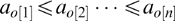
Order the requests in increasing order of earliest starting times. That is, find o[1], o[2],…, o[n] such that

Step 4: :

Initialize the current request to the first in the above order. That is, put k ← 1 and K ← o[k]

Step 5: :

Set the current request to the next in the above order. That is, put k ← k+1 and K ← o[k].

Step 6: :

For the current request, find its earliest immediate predecessor. That is, find smallest j such that if a _i ⩽a _j ⩽a _k and requests i and j are not mutually exclusive alternates, then

and

Denote such j as ĵ.

Step 7: :

Set the latest time a request can start such that it ends before the earliest starting time of the current request. That is,

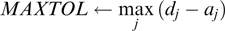
Step 8: :

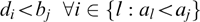
Include in the immediate predecessor set of the current request PRED _o[k], every request l such that a _l >a _ĵ which satisfies the following conditions:

a. Latest ending time is greater than the latest possible start time of its predecessors which was calculated in Step 7 (Theorem 1). That is, d _o[l]>LPT _o[k].

b. Requests o[l] and o[k] are not mutually exclusive alternates.

c. Latest ending time not greater than the earliest starting time of the current request plus the maximum band length. That is, d _o[l]⩽a _o[k]+MAXTOL.

d. The earliest starting time not greater than the begin time of the current request. That is, a _o[l]⩽a _o[k].

e. Earliest end time not greater than the latest start time of the current request (Theorem 3). That is, c _o[l]⩽b _o[k].

Step 9: :

If k⩽n, go to Step 5; otherwise stop.

A.2. Heuristic for sequencing requests

Step 1: :

Initialize the On-Schedule-Flags to zero for all requests. That is, put FLAG _j ← 0 for all j.

Step 2: :

Set the schedule generation period begin time to the earliest starting time of all the bands. That is, put SGB ← min _j a _j .

Step 3: :

Set the schedule generation period end time to the latest ending time. That is, put SGE ← max _j d _j .

Step 4: :

Define a fictitious request to represent the schedule period begin time. Set its duration to a small value, for example, 0.1. Set its earliest starting time to the schedule generation period begin time minus the small value. Set its latest ending time to the schedule generation period begin time. That is, put p ₀ ← 0.1, d ₀ ← SGB, c ₀ ← SGB, a ₀ ← SGB–0.1, and b ₀ ← SGB–0.1.

Step 5: :

Define a fictitious request to represent the schedule period end time. Set its duration to a small value, for example, 0.1. Set its earliest starting time to the schedule generation period end time minus the small value. Set its latest ending time to the schedule generation period end time plus the small value. That is, put p _n+1 ← 0.1, a _n−1 ← SGE, b _n−1 ← SGB, d _n+1 ← SGB+0.1, and c _n+1 ← SGB+0.1.

Step 6: :

Set the benefit associated with each request. The appropriate benefit for a request is the duration of the request if the objective is to maximize the total time scheduled. The appropriate benefit is 1 if the objective is to maximize the number of events scheduled. That is,

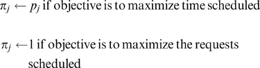
(Note that π _j has value 0 for fictitious requests, and value equal to that of the original request if j is an artificial mutually exclusive alternate.)

Step 7: :

Determine the set of immediate predecessor requests for each request using the above procedure. That is, determine PRED _j for each j. (Note that since a fictitious request is added and it can precede any request, PRED _j is not empty for any j.)

Step 8: :

Order the requests in increasing order of earliest starting times and, in case of ties, in increasing order of latest ending times. That is, find o[1], o[2], …, o[n] such that

and

(Note that n is the number of the original requests plus the number of mutually exclusive alternates created for each original request. In addition, there are two fictitious requests giving a total of n+2. However, the index of the first and last fictitious requests are zero and n+1, so the request indices are 0, 1,…,n+1.)

Step 9: :

Initialize the end time and the maximum cumulative benefit realized through the completion of an event for the schedule generation period begin time fictitious request. That is, put f ₀ ← SGB and z ₀ ← 0.

Step 10: :

Set the current request to the first request in the above order. That is, put k ← 1 and K ← o[k].

Step 11: :

Set the current request to the next request in the above order. That is, put k ← k+1 and K ← o[k].

Step 12: :

Determine the maximum cumulative benefit and the optimal predecessor for the current request using the following algorithm. Define

z _j as the maximum cumulative benefit realized through completion of the event for request j,

f _j as the end time of the event for request j,

PRED _j as the set of predecessors for request j,

OPT(j) as the optimal predecessor for request j.

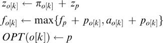
Find p∈PRED _o[k] to maximize z _o[k] such that

(i) f _p ⩽b _o[k],

(ii) the optimal predecessor chain for request

 p does not include a mutually exclusive

alternate for the current request,

(iii) p<o[k] (to make sure that z _p is already

 defined).

Then put

Step 13: :

If k⩽n, go to Step 11.

Step 14: :

Set the current request to the fictitious request representing the schedule generation period end time. That is, put k ← n+1.

Step 15: :

Calculate the earliest starting time of the effective band for the current request. That is, put EFF(a _k ) ← f _n+1–p _n+1.

Step 16: :

Calculate the latest ending time of the effective band for the current request. That is, put EFF(d _k ) ← f _n+1.

Step 17: :

Initialize the earliest starting time of the effective band of the immediate successor request. That is, put BSUCCR ← EFF(a _k ).

Step 18: :

Find the optimal immediate predecessor of the current request. That is, put p ← OPT(k).

Step 19: :

Go to Step 26 if the optimal immediate predecessor of the current request is the schedule generation period begin time fictitious request. That is, go to Step 26 if p=o[0].

Step 20: :

Set the On-Schedule-Flag for the optimal immediate predecessor of the current request to 1. That is, put FLAG _j ← 1.

Step 21: :

Set the earliest starting time of the effective band for the optimal immediate predecessor of the current request. That is, put EFF(a _p ) ← f _p –p _p .

Step 22: :

Set the latest ending time of effective band for the optimal immediate predecessor of the current request. That is, put EFF(d _p ) ← min{d _p , BSUCCR}.

Step 23: :

Reset the earliest starting time of the effective band of the immediate successor request. That is, put BSUCCR ← EFF(a _p ).

Step 24: :

Set the current request to its optimal immediate predecessor. That is, put k ← p.

Step 25: :

Go to Step 18.

Step 26: :

Stop. The sequence of scheduled requests described by On-Schedule-Flags and the effective bands define the schedule.

References

Arbabi M (1984). Range scheduling automation. IBM Technical Directions 10: 57–62.
Arbabi M and Pfeifer M (1987). Range and mission scheduling automation using combined AI and operations research techniques. In: Griffin S (ed). First Annual Workshop on Space Operations Automation and Robotics (SOAR ‘87): NASA Conference Publication 2491. Washington. DC, pp 315–320.
Reddy SC and Brown WL . Single processor scheduling with job priorities and arbitrary ready and due times. Working paper, October 1986, Computer Sciences Corporation. Beltsville, MD.
Cheng TCE and Sin CCS (1990). A state-of-the-art review of parallel-machine scheduling research. Eur J Opl Res 47: 271–292.
Gensch DH (1978). An industrial application of the traveling salesman's subtour problem. AIIE Trans 10: 362–370.
Butt SE and Cavalier TM (1994). A heuristic for the multiple tour maximum collection problem. Comput Opns Res 21: 101–111.
Kataoka S and Morito S (1988). An algorithm for single constraint maximum collection problem. J Opns Res Soc Japan 31: 515–530.
Golden BL, Levy L and Dahl R (1981). Two generalizations of the traveling salesman problem. Omega 8: 439–441.
Balas E (1989). The prize collecting traveling salesman problem. Networks 19: 621–636.
Golden BL, Levy L and Vohra R (1987). The orienteering problem. Nav Res Logist Q 34: 307–318.
Reddy SD (1988). Scheduling of tracking and data relay satellite system (TDRSS) antennas: scheduling with sequence dependent setup times. Presented at ORSA/TIMS Joint National Meeting, Denver, CO.
Gabrel V (1995). Scheduling jobs within time windows on identical parallel machines: new model and algorithms. Eur J Opl Res 83: 320–329.
Randhawa SU and Kuo CH (1997). Evaluating scheduling heuristics for non-identical parallel processors. Int J Prod Res 35: 969–981.
Tsiligirides T (1984). Heuristic methods applied to orienteering. J Opl Res Soc 35: 797–809.
Laporte G and Martello S (1990). The selective traveling salesman problem. Discrete Appl Math 26: 193–207.
Ramesh R and Brown KM (1991). An efficient four-phase heuristic for the generalized orienteering problem. Comput Opns Res 18: 151–165.
Ramesh R, Yoon YS and Karwan MH (1992). An optimal algorithm for the orienteering tour problem. ORSA J Comput 4: 155–165.
Kantor MG and Rosenwein MB (1992). The orienteering problem with time windows. J Opl Res Soc 43: 629–635.
Feo TA and Resende MGC (1995). Greedy randomized adaptive search procedures. J Glob Optimiz 6: 109–133.
Rojanasoonthon S and Bard JF (2001). A grasp for parallel machine scheduling with time windows. Working Paper, 2001, Graduate Program in Operations Research. University of Texas, Austin, TX.
Or I . Traveling salesmen-type combinatorial problems and their relation to the logistics of blood banking. PhD thesis, 1976, Department of Industrial Engineering and Management Sciences, Northwestern University, Evanston, IL.
Rojanasoonthon S . Parallel machine scheduling with time windows. PhD thesis, 2003. Graduate Program in Operations Research and Industrial Engineering, University of Texas, Austin, TX.
Dodd JC and Reddy SD . The scheduling technology in the NASA TDRSS network control center (NCC). AAS paper, October 1987, Computer Sciences Corporation. Beltsville, MD.
Author information
Authors and Affiliations
Corresponding author