
Abstract
This paper presents the bounds of exotic options, namely compound options, barrier options and Asian options. There are two purposes of this study: first, option price bounds are used to reveal much insightful information regarding the distinctive characteristics of exotic options, which help to understand those complex derivatives; second, although the bounds of vanilla options have been long recognized, there is no such development for exotic options. This paper aims to fill the gap.
INTRODUCTION
The bounds on option prices provide a range of possible values of options, place restrictions that narrow the search of exact option prices and provide many insightful perspectives about option prices. For example, by comparing the lower bounds of Asian options and vanilla options, Ye1, 2 shows that an Asian option can be more expensive than a similar plain vanilla European option. This finding corrects a commonly accepted misconception that Asian options are always cheaper than their plain vanilla counterparts.
The bounds on plain vanilla options have been extensively studied in the literature. For instance, Merton3 derived the upper and lower bounds on plain vanilla options based on a no-arbitrage argument. Perrakis and Ryan,4 Ritchken5 and Levy,6 among others, improved Merton's bounds by imposing more restrictive assumptions. However, little effort has been made in the literature to derive bounds on exotic options. This paper aims to fill the gap.
Although the no-arbitrage argument is useful in deriving plain vanilla option bounds, it is intractable to extend this approach to exotic options, because of the difficulty of constructing arbitrage strategies given the complex structures of exotic options. Instead, we derive bounds by incorporating the property that option values are monotonic in volatility. That is, for example, if the value of an option is monotonically increasing in the volatility of the underlying asset, the limit price as the volatility goes to zero is a lower bound of the option price.
ASSUMPTIONS
For simplicity, we assume that the underlying asset of an option is a stock paying a continuous dividend yield, q. We assume that the market is perfect. Transaction costs and taxes are ignored. The interest rate is constant over time and has a flat term structure.
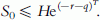
Let S t be the stock price at time t, 0⩽ t⩽ T, σ the volatility of the stock price and r the risk-free interest rate with continuous compounding.
As σ → 0, it yields

for any t>0.
The behaviours of plain vanilla European option prices as σ → 0 have been extensively studied in the literature. For example, Kolb7 shows that the price of a plain vanilla European option on a risk-free stock is equal to the lower bound that is derived by Merton by using the no-arbitrage argument. The lower bounds on plain vanilla European call and put with a strike price K and time to maturity T can be written as follows:


In the following sections, we derive the bounds for compounded options, barrier options and Asian options.
COMPOUND OPTIONS
The underlying asset of a compound option is an option, called the underlying option. Compound options include compound calls and compound puts.
Let K and T be the strike price and time to maturity of a compound option, and K* and T* the strike price and time to maturity of the underlying option, with T*>T>0. For convenience, we use the following notations:


To avoid trivia, we assume that  . Let C(t) and P(t) denote the value of the underlying option, call or put, at time t.
Bounds on compound puts
Compound puts include a put on a call and a put on a put. Compound puts have a very distinctive characteristic: the value of a compound put decreases as the volatility of the underlying stock price increases, in contrast to most options. This is because an increase in the volatility will increase the value of the underlying option, which, in turn, will reduce the value of the compound put. Consequently, as the volatility goes to zero, the limit value of a compound put provides an upper bound of the option, rather than a lower bound.
A put on a call
Let PC(t) be the values of a call on a call at time t. By definition, the payoff of a put on a call at t=T is as follows:

As σ → 0, C(T) is equal to the lower bound of the call. Thus, from equations (1) and (2), we have

This yields the upper bound of a put on a call as follows:

which is plotted in Figure 1(a).

Bounds of compound options.Notes: S 0 is the current market price of the underlying stock. q is the dividend yield of the stock. k and k * are defined as k=Ke−rT and k *=K *e−rT*, k *>k, where K and T are the strike price and time to maturity of a compound option, K * and T * are the strike price and time to maturity of the underlying option, and r is the risk-free rate of interest with continuous compounding, q is the continuous dividend yield of the underlying stock. (a) A put on a call. (b) A put on a put. (c) A put on a call. (d) A put on a put.
Noting that zero is the lower bound of an option, it follows from equation (4) that PC=0 when  . This indicates that if the underlying put is deep in-the-money, the value of a compound option is zero. In other words, a put on a call will be worth nothing if the underlying stock price exceeds a certain level. In particular, if the underlying stock is not expected to pay dividends during the life of the options, the price of a put on a call is zero when the stock price is greater than the sum of the strike prices of the compound option and the underlying option.
A put on a put
Let PP ( t) be the values of a call on a call at time t. By definition, the payoff of a put on a call at t=T is as follows:

From equations (1) and (3), as σ → 0, it yields

This yields the upper bound of a put on a put as follows:

which is plotted in Figure 1(b).
As zero is a lower bound of an option, it follows from equation (5) that PP=0 when  . This indicates that a put on a put will be worth nothing if the underlying stock price is below a certain level. In particular, if the underlying stock is not expected to pay dividends during the life of the options, the price of a put on a put is zero when the stock price is lower than the difference between the present value of the strike price of the underlying put and the present value of the strike price of the compound option. Noting that
  is usually much greater than
  , a put on a put can be worthless for quite a large range of stock price.
Bounds on compound calls
Compound call options include a call on a call and a call on a put. As a decrease in the volatility decreases the value of the underlying option, it also decreases the value of a compound call. Thus, as the volatility goes to zero, the limit value of a compound call provides a lower bound of the option. As the derivation of the lower bounds on compound calls is similar to that of the upper bounds on compound puts, we will only provide results below.
A call on a call
The lower bound of a call on a call is as follows:

As the value of the underlying call at time T cannot be higher than S T e−q(T*–T), the upper bound of the compound call is

The bounds given by equations (6) and (7) are plotted in Figure 1(c).
A call on a put
The lower bound of a call on a put as follows:

As the value of the underlying put at time T cannot be higher than  , the upper bound of the compound call is

The bounds given by equations (8) and (9) are plotted in Figure 1(d).
BARRIER OPTIONS
Barrier options include knock-out options and knock-in options. A knock-out option is a regular option that ceases to exist if the asset price reaches a pre-set barrier; a knock-in option is a regular option that comes into existence only if the asset price reaches a pre-set barrier. We denote the barrier by H.
As the value of a knock-out option may not be monotonic in volatility, as pointed out by Nelken,8 our volatility approach cannot be used to derive the bounds for knock-out options. Thus, we limit our discussion to knock-in options the values of which are monotonically increasing in volatility.
Up-and-in options
For up-and-in options, we have H>S 0. Noting that the case of r⩽q is trivial where the lower bound is zero, we limit our discussion to the case of r>q, in which, as σ goes to zero, the stock price becomes monotonic increasing in time.
Up-and-in call
To avoid trivia, we assume that H>K, because otherwise an up-and-in call is equivalent to a vanilla call.
Let LB UIC denote the lower bound of an up-and-in call option. As σ goes to zero, we consider two possible situations:
Case 1:
-
 Equation (1) implies that S
T
⩽H. This means that the barrier will not be reached during the life of the option. Thus, the lower bound of the up-and-in call is zero, that is,
Equation (1) implies that S
T
⩽H. This means that the barrier will not be reached during the life of the option. Thus, the lower bound of the up-and-in call is zero, that is,


Case 2:
-
 . Equation (1) implies that S
T
> H. This means that the barrier will be reached and the option becomes a vanilla European call before the expiration date of the option. Thus, the lower bound of the up-and-in call is the same as one of the vanilla European call, as follows:
. Equation (1) implies that S
T
> H. This means that the barrier will be reached and the option becomes a vanilla European call before the expiration date of the option. Thus, the lower bound of the up-and-in call is the same as one of the vanilla European call, as follows: 
 .
. 
However, as we assumed that  and H>K, we have S
0e−qT>Ke−rT. It yields
and H>K, we have S
0e−qT>Ke−rT. It yields

To summarise, a lower bound for an up-and-in call is as follows:

which is plotted in Figure 2(a) where r>q, H>K and S 0<H .

Bounds of barrier options. Notes: S 0 is the current market price of the underlying stock. q is the dividend yield of the stock. H, K and T are the barrier, strike price and time to maturity of a barrier option, respectively. r is the risk-free rate of interest with continuous compounding. (a) Up-and-in calls (r>q, H>K). (b) Up-and-in puts (r>q, H<K). (c) Down-and-in calls (r<q, H>K). (d) Down-and-in puts (r<q, H<K).
In contrast to vanilla options, Figure 2(a) shows that the lower bound of an up-and-in call is discontinuous at S 0 =He−(r−q)T. As option prices are close to the lower bound, especially when the volatility is small, this discontinuity indicates that the delta can be very high around the area, which makes it difficult to hedge.
Up-and-in puts
Let LB UIP denote the lower bound of an up-and-in put option. Similar to up-and-in calls, as σ goes to zero, we consider two possible situations:
Case 1:
-
S 0 ⩽He−(r−q)T. As the barrier will not be reached during the life of the option, the lower bound of the up-and-in put is


Case 2:
-
S 0>He−(r−q)T. The barrier will surely be reached. Thus, the option becomes a vanilla European put before the expiration date of the option. Therefore, the lower bound of the up-and-in put is the same as one of the vanilla European put, as follows:


If K⩽H, then Ke−rT<He−rT<S 0e−qT. This results in LB UIP =0. By combining Case 2 with Case 1, the lower bound is zero for all possible values of S 0.
If K>H, by combining Case 1, the lower bound of the up-and-in put is as follows:

which is plotted in Figure 2(b) where r>q, K>H and S 0<H.
Figure 2(b) shows that the lower bound of an up-and-in put is not a monotonic function of stock price. Instead, the lower bound jumps up at S 0 =He−(r−q)T, then decreases as the stock price increases. This is consistent with the fact that the value of an up-and-in put increases before the barrier is reached, as an increase in stock price increases the possibility that the barrier will be hit, and then decreases after the barrier is reached because now the option becomes a regular put.
Note that if K>He−(r–q)T, equation (11) is truncated and becomes:

Down-and-in options
For down-and-in options, we have H<S 0. Noting that the case of r⩾q is trivial where the lower bound is zero, we limit our discussion to the case of r<q, in which, as σ goes to zero, the stock price becomes monotonic decreasing in time. As the derivation is similar to that for up-and-in options, we will only present results for down-and-in options.
Let LB DIC and LB DIP denote the lower bounds of down-and-in call and down-and-in put, respectively.
Down-and-in calls
If H⩽K, the lower bound of a down-and-call is zero. However, if H>K, the lower bound of a down-and-in call is as follows:

where r<q, S 0>H>K.
Down-and-in puts
If the barrier is above the strike price, a down-and-in put is equivalent to a vanilla put. To avoid trivia, we assume that H<K. The lower bound of a down-and-in put is

where r<q, H<K and S 0>H. The lower bounds of down-and-in call and down-and-in put are plotted in Figures 2(c) and (d), respectively.
ASIAN OPTIONS
Asian options are options the payoffs of which depend on the average of the stock price over time. There are many variants of Asian options. Given the page limit, and because the bounds of fixed-strike arithmetic average price options have been presented in Ye,1, 2 this paper focuses on the bounds of floating-strike arithmetic average price options, in which the average price is defined as follows:

where S n is the underlying stock price at time t n =nΔt, with Δt=T/N, N represents the number of samples used for calculating the average price, and T is the expiration date of an Asian option. For simplicity, the following notations are used:


A floating-strike arithmetic average price option is similar to a vanilla option, with its strike price being replaced by the arithmetic average price, S ave . Let LB AC and LB AP be the lower bounds of the Asian call and Asian put, respectively. As σ → 0, we can have the lower bounds of the Asian options as follows:


If r>q, from equation (15) it can be shown that

Thus, the lower bounds of the Asian options are as follows:


In contrast, if r<q, then G>R/Q, and the lower bounds of the Asian options are as follows:


These bounds for Asian call when r>q and Asian put when r<q are plotted in Figures 3(a) and (b), respectively.

Lower bounds of Asian options and vanilla European options.Notes: S 0 is the current market price of the underlying stock, T is the time to maturity of options, K is the strike price of vanilla options, R, Q and G are defined by equation (16). (a) Floating strike average calls (r>q). (b) Floating strike average calls (r>q).
The figure presents several very distinctive characteristics: first, the lower bounds are linear to initial stock price, S 0, whereas the lower bounds of most options are non-linear; second, not only the lower bounds for Asian calls, but also the lower bounds for Asian puts are increasing in stock price; third, the lower bounds are positive for any positive stock price.
In order to make comparisons, the lower bounds of vanilla European calls and puts are also plotted in Figures 3 (a) and (b), along with their Asian counterparts. From the figure, we can see that, in the case of r>q, the lower bound of an Asian call is higher than the lower bound of its vanilla counterpart when S 0<K/G. This implies that, when S 0<K/G and the volatility is lower than a certain level, the value of a vanilla European call is lower than the lower bound of Asian calls. Thus, Asian calls can be more expensive than their vanilla European counterparts. In the case of r<q, the lower bound of an Asian put is higher than the lower bound of its vanilla counterpart when S 0>K/G. Reasoning similarly, we can conclude that Asian puts can be more expensive than their vanilla European counterparts. This contradicts a commonly accepted notion that Asian options are cheaper than their vanilla counterparts, in the case of floating-strike arithmetic average price options, whereas a similar result was presented in Ye1, 2 in the case of fixed-strike arithmetic average price options.
CONCLUSIONS
This paper presents the bounds on compound options, barrier options and Asian options. By examining these bounds, we learned many interesting and distinctive features of exotic options. For examples, the upper and lower bounds of compound puts will merge into zero for a certain range of the underlying stock prices, which implies that the value of a compound put is exactly equal to zero when the stock price is within the range; the lower bounds of knock-in options show discontinuity in the underlying stock price, which suggests that the delta of a compound put can be extremely high; the lower bound of an Asian option can be above the lower bound of its vanilla counterpart, which implies that Asian options can be more expensive than their vanilla counterparts, contrary to a common notion. Although only a small number of exotics and their applications are presented in this paper, our future research will explore more potential applications of those bounds and develop bounds of other exotic options.
References
Ye, G. (2005) Asian options can be more expensive than plain vanilla counterparts. Journal of Derivatives 13 (1): 56–60.
Ye, G. (2008) Asian options versus vanilla options: A boundary analysis. Journal of Risk finance 9 (2): 188–199.
Merton, R. (1973) Theory of rational option pricing. Bell Journal of Economics and Management Science 4: 141–183.
Perrakis, S. and Ryan, P. (1984) Option pricing bounds in discrete time. Journal of Finance 39: 519–527.
Ritchken, P. (1985) On option pricing bounds. Journal of Finance 40: 1219–1233.
Levy, H. (1985) Upper and lower bounds of put and call option value: Stochastic dominance approach. Journal of Finance 40: 1197–1217.
Kolb, R. (2007) Futures, Options, and Swaps, 5th edn., Blackwell Publishing, Malden, MA, p. 430.
Nelken, I. (1999) Pricing, Hedging, and Trading Exotic Options. NY: McGraw-Hill, p. 139.
Author information
Authors and Affiliations
Corresponding author
Additional information
Practical applications Exotic options are very powerful and widely used tools of risk management. However, because of the complexity of those contracts, the basic characteristics of many exotic options are not clearly understood, or are even misunderstood. Although most researches have been focused on developing models for pricing exotic options, it is important to study their unique characteristics and to understand them correctly. In addition, as the exact valuations of exotic options are usually difficult, it is useful to narrow the searching of the prices by placing boundary restrictions.
Rights and permissions
About this article
Cite this article
Ye, G. Exotic options: Boundary analyses. J Deriv Hedge Funds 15, 149–157 (2009). https://doi.org/10.1057/jdhf.2009.5
Received:
Revised:
Published:
Issue Date:
DOI: https://doi.org/10.1057/jdhf.2009.5