
Abstract
Shrunk sample covariance matrix is a factor model of a special form combining some (typically, style) risk factor(s) and principal components with a (block-)diagonal factor covariance matrix. As such, shrinkage, which essentially inherits out-of-sample instabilities of the sample covariance matrix, is not an alternative to multifactor risk models but one out of myriad possible regularization schemes. We give an example of a scheme designed to be less prone to said instabilities. We contextualize this within multifactor models.
Notes
Deliberately omitting many important details, that is.
Albeit, some elements of ‘risk management’ can be (and at times are) incorporated into the expected returns, for example, sector or industry neutrality.
Let R is be the time series of our returns, i=1, …, N, s=0, 1, …, M. Let
 be the serially demeaned returns, where
  is the time-series mean of R
is
. In matrix notation SCM is given by C=(1/M)XXT. (We are assuming M≫1, so the difference between the unbiased estimate with M in the denominator versus the maximum likelihood estimate with M+1 in the denominator is immaterial for our purposes). Since at most M columns of the matrix X are linearly independent (as its column sums ∑s=0MX
is
=0), the rank of the matrix C
ij
is at most M if M<N.
is the time-series mean of R
is
. In matrix notation SCM is given by C=(1/M)XXT. (We are assuming M≫1, so the difference between the unbiased estimate with M in the denominator versus the maximum likelihood estimate with M+1 in the denominator is immaterial for our purposes). Since at most M columns of the matrix X are linearly independent (as its column sums ∑s=0MX
is
=0), the rank of the matrix C
ij
is at most M if M<N.This statement is often regarded as stemming from empirical evidence. However, it is well-understood theoretically. We can always rotate our serially demeaned returns X is to an orthogonal basis and rescale them to have unit serial variances. Then the true covariance matrix is the N × N identity matrix. Pursuant to the Bai-Yin theorem (Bai and Yin, 1993), the smallest and largest eigenvalues of SCM have the limits
 and
and 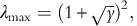 where y=N/M is fixed and N, M→∞. So for M, N≫1 we must have M≫N for all eigenvalues to be close to 1.
These are typically, but not necessarily, style factors.
In the model with uniform correlations used in (Ledoit and Wolf, 2004) we have Δ ij =ρσ i σ j for i≠j, where σ i 2=C ii . This is a special case of a 1-factor model Δ ij =ξ i 2δ ij +Ω i Ω j with ξ i 2=(1−ρ) σ i 2, Ω i 2=ρ σ i 2 and the 1 × 1 factor covariance matrix absorbed into Ω i .
See, for example, (Grinold and Kahn, 2000) and references therein.
Also, we are assuming that there are no pairwise 100 per cent (anti-)correlated returns.
In practice these null eigenvalues can be distorted by computational rounding and turn into small positive or negative values. So, we assume that all such ‘quasi-null’ eigenvalues are rounded to 0. Furthermore, this assumes that there are no N/As in any of the time series of returns. If there are (non-uniform) N/As and SCM is computed by omitting such pair-wise N/As, then the resulting correlation matrix can have negative eigenvalues that are not ‘small’ in the above sense, that is, they are not zeros distorted by computational rounding. In this case we can use the deformation method of Rebonato and Jäckel (1999). In any event, we assume that all λ(a)⩾0.
This can also be understood using the Bai-Yin theorem (see note 6): the limit for the largest eigenvalue
 holds even if y=N/M>1. So, the first principal component is relatively stable, but higher ones are not as constrained and tend to be less stable.
 be the serially demeaned returns, where
  is the time-series mean of R
is
. In matrix notation SCM is given by C=(1/M)XXT. (We are assuming M≫1, so the difference between the unbiased estimate with M in the denominator versus the maximum likelihood estimate with M+1 in the denominator is immaterial for our purposes). Since at most M columns of the matrix X are linearly independent (as its column sums ∑s=0MX
is
=0), the rank of the matrix C
ij
is at most M if M<N.
is the time-series mean of R
is
. In matrix notation SCM is given by C=(1/M)XXT. (We are assuming M≫1, so the difference between the unbiased estimate with M in the denominator versus the maximum likelihood estimate with M+1 in the denominator is immaterial for our purposes). Since at most M columns of the matrix X are linearly independent (as its column sums ∑s=0MX
is
=0), the rank of the matrix C
ij
is at most M if M<N. and
and  where y=N/M is fixed and N, M→∞. So for M, N≫1 we must have M≫N for all eigenvalues to be close to 1.
 holds even if y=N/M>1. So, the first principal component is relatively stable, but higher ones are not as constrained and tend to be less stable.
References
Bai, Z.D. and Yin, Y.Q. (1993) Limit of the smallest eigenvalue of a large dimensional sample covariance matrix. The Annals of Probability 21 (3): 1275–1294.
Grinold, R.C. and Kahn, R.N. (2000) Active Portfolio Management, New York: McGraw-Hill.
Kakushadze, Z. (2015) Russian-doll risk models. Journal of Asset Management 16 (3): 170–185.
Ledoit, O. and Wolf, M. (2004) Honey, I shrunk the sample covariance matrix. The Journal of Portfolio Management 30 (4): 110–119.
Markowitz, H. (1952) Portfolio selection. The Journal of Finance 7 (1): 77–91.
Menchero, J. and Mitra, I. (2008) The structure of hybrid factor models. Journal of Investment Management 6 (3): 35–47.
Rebonato, R. and Jäckel, P. (1999) The most general methodology to create a valid correlation matrix for risk management and option pricing purposes. Working Paper, http://ssrn.com/abstract=1969689.
Sharpe, W.F. (1966) Mutual fund performance. Journal of Business 39 (1): 119–138.
Sharpe, W.F. (1994) The Sharpe ratio. The Journal of Portfolio Management 21 (1): 49–58.
Author information
Authors and Affiliations
Corresponding author
Additional information
Disclaimer: This address is used by the corresponding author for no purpose other than to indicate his professional affiliation as is customary in publications. In particular, the contents of this article are not intended as an investment, legal, tax or any other such advice, and in no way represent views of Quantigic® Solutions LLC, the website www.quantigic.com or any of their other affiliates.
1received his PhD in theoretical physics from Cornell University, was a Postdoctoral Fellow at Harvard University and an Assistant Professor at the C.N. Yang Institute for Theoretical Physics at Stony Brook. He received the Alfred P. Sloan Fellowship in 2001. After expanding into quantitative finance, he was a Director at RBC Capital Markets, Managing Director at WorldQuant, Executive Vice President and substantial shareholder at Revere Data, Adjunct Professor at UConn and currently is the President and co-owner of Quantigic® Solutions and a Full Professor at Free University of Tbilisi. He has 100+ publications in physics and finance.
Rights and permissions
About this article

Cite this article
Kakushadze, Z. Shrinkage=factor model. J Asset Manag 17, 69–72 (2016). https://doi.org/10.1057/jam.2015.40
Received:
Revised:
Published:
Issue Date:
DOI: https://doi.org/10.1057/jam.2015.40