The Impact of Disaster Relief on Economic Growth: Evidence from China

Abstract

In this paper we construct a simple two-period equilibrium model for analysing the impact of post-disaster transfer payments on economic growth. This model can be used to show that direct payment of disaster relief funds may aggravate rather than mitigate the negative impact of disasters on the economy. The substitution effect of direct transfer payment depresses post-disaster labour supply and hence economic growth. This conclusion from the theoretical model is tested using Chinese provincial panel data and applying generalised method of moments (GMM) system estimation. The empirical analysis largely confirms the theoretical predictions. In China, post-disaster transfer payments are indeed found to exacerbate the negative impact of disasters on economic growth. Therefore, we suggest that relief should be oriented to create work incentive in order to avoid its depressing effect on economic growth.

Introduction and literature review

Natural disasters are one of the most serious external threats to sustainable economic development. On the one hand, they have a high human cost in terms of casualties that affect demand, labour supply and social stability. On the other hand, these economic losses hurt capital stock and subsequent production. China is a country that has experienced some of the most serious natural disasters in recent years, the frequency of which has increased significantly. As a consequence, both the population affected and the economic losses incurred have greatly increased. According to the database maintained by the Centre for Research on the Epidemiology of Disasters (CRED) at the Catholic University of Louvain in Belgium, China experienced the highest frequency of natural disasters during the last decade since 1900, when they were first recorded, accounting for 37 per cent of total occurrences since then.¹ In terms of population affected and economic loss, the share of the last decade is even as high as 50 per cent (see Table 1). Especially after the 2008 earthquake in China's Sichuan province and the 2011 tsunami in Japan, there has been a renewed interest on the part of economists both in China and abroad in studying the impact of natural disasters on economic growth.

Table 1 Natural disasters of the past decade in China relative to the period 1900–2012, in per cent

Most of the discussion has focused on disaster preparedness and prevention, while post-disaster macroeconomic development has received rather little attention.² An early exception is Hirshleifer,³ who undertook research into post-disaster development in his analysis of Western Europe after the onslaught of the Black Death in the 14^th century. Distinguishing between short-term and long-term effects, he noted that the short-term economic impact of the Black Death was in line with economic theory, namely a slowdown of production, changed distribution of income (workers’ wages rose, while capitalists’ returns fell), and even political disintegration. However, he did not believe the Black Death to be the primary reason for the observed drop in European economic output and was not willing to conclude that natural disasters inevitably lead to economic recession and its consequences for society. Changes in social networks are another important aspect of post-disaster development. Chang⁴ argues that community cohesion may have been strengthened by flooding in China, without, however amounting to a full substitute of outside assistance for economic recovery.

Some of the early empirical work applying econometric techniques examined changes in macroeconomic data after the occurrence of a disaster, such as a country's GDP, rate of inflation, balance of payments and general financial situation.⁵ More recently, advanced econometric methods have been applied to data of developed countries in an attempt to identify factors that magnify and mitigate, respectively, the effect of natural disasters on economic growth.⁶ In fact, some of the authors have found natural disasters to be a source of “creative destruction” promoting economic growth.⁷

In economic theory, there does not yet exist a theoretical framework for modelling the links between natural disasters and economic growth. Attempts at building a partial model, mainly by Anbarci and Escaleras,⁸ revolved around the collective nature of efforts designed to reduce losses due to earthquakes. Hallegatte et al.,⁹ extending Solow's model,¹⁰ specified a non-equilibrium dynamic model for analysing the macroeconomic impact of severe climate change. Wang¹¹ built a two-sector endogenous growth model subject to natural disasters, with long-term growth depending mainly on the loss of human rather than physical capital. McDermott¹² and Barry,¹³ based on the Solow model once more, introduced credit constraints, pointing out that these reflect the level of development rather than the acceleration or deceleration in economic growth caused by natural disasters.

In sum, it is fair to say that research on the impact of natural disasters on economic growth is still in its infancy, with limited connection to the development literature.

This study seeks to establish this connection, with particular emphasis on disaster relief. It examines whether disaster relief enhances economic growth, thus contributing to a rise in the standard of living, or whether it actually serves to depress labour supply and magnify the negative impact of disasters on the economy. The country to be analysed is China, where post-disaster assistance provided by the central government and by communities in the guise of donations is increasingly becoming the subject of debate. These types of assistance are suspected of being open to corruption and misappropriation of funds due to a lack of governance. Therefore, government relief and community donations may not be the best way to deal with disasters. In keeping with the adage, “Teaching a man to fish, rather than giving him a fish”, it might be preferable to create work incentives designed to foster post-disaster activities that contribute to GDP and employment.

The remainder of this paper is organised as follows. The second section contains a simple two-period equilibrium model that includes both post-disaster transfer payments and investments. The third section is devoted to testing the theory using the data from China, while the fourth section offers a summary and conclusions.

Theory

The theoretical model is inspired by the work of Barry13 and McDermott.12 In the first period, natural disaster causes a loss both in capital stock and labour supply (due to injuries or casualties). In the second period, consumers in disaster-hit areas receive a one-time transfer payment covering their cost of living during the post-disaster period.¹⁴ The following subsection presents the basics of this model.

The basic model

Consumers are assumed to maximise a utility function given by

The level of utility attained thus depends on consumption C₁ and C₂ in periods 1 and 2 and leisure (H–L₁) and (H–L₂), respectively, where H denotes the time available for work per period while L₁ and L₂ symbolise labour supply. The disaster causes a reduction in H and therefore labour supply, ceteris paribus. In the second period, consumers receive transfer payments amounting to Tr. It is important to note that Tr is used for consumption, serving as a perfect substitute for C₂, which is the decision variable of interest. B<1 reflects the rate of time preference. The utility weight of consumption share α satisfies 0<α<1. The inter-temporal budget constraint is therefore:

where R<1 is the discounting factor.¹⁵ The production function F has capital and labour as its arguments, with K₁ denoting the initial capital stock of the economy and I is the personal investment in the first period. Following Barry,13 it is assumed that additional new capital must become available in the first period to be productive in the second period. However, depreciation is neglected for simplicity. Investment entails a sacrifice of consumption during the first period, which means saving can be fully transferred to investment. For simplicity once more, we assume that there is no government investment and therefore I can be taken to directly affect the rate of economic growth. Indeed, I will be interpreted as the growth rate, neglecting issues surrounding its (potentially changing) marginal efficiency. Accordingly, the impact of a disaster on economic growth is analysed through its effect on I.¹⁶

The first-order conditions of this maximisation problem are¹⁷

Equations (1) and (4) represent the inter-temporal efficiency conditions for the consumption and investment decisions, respectively.¹⁸ Eqs. (2) and (3) are the inter-temporal efficiency conditions relating to the relationship between leisure and consumption. F _Li and F _Ki represent the marginal product of labour and of capital, respectively. Capital stock of each period satisfied K₂=K₁+I (Investment).

The market-clearing conditions read,¹⁹

The impact of disaster relief on post-disaster investment

A natural disaster hitting the economy in the first period has two effects. First, the capital stock is destroyed, that is, dK₁<0. Second, the potential supply of labour is impaired, due to injuries and casualties or due to the disruption of production processes because workers cannot reach their workplaces or lack important intermediate goods, that is, dH<0. In order to obtain definite results, the production function is assumed to be of the Cobb–Douglas form (0<β<1) with constant returns to scale and no technological change,²⁰

After substitution into (1)–(6), this results in the following expression for optimal second-period labour supply and investment, respectively²¹:

where A₁=α(1−β)(βR)^1/(1−β)/(1−αβ), A₂=(1−α)βR/(1−αβ).

Proposition 1:

• All else equal,

• 1) A decline in the initial capital stock is fully compensated by investment, that is, ∂I/(−∂K₁)=1;

• 2) A decline in the potential supply of labour depresses investment, that is ∂I/∂H=A₁0 since A₁0 (note that 0<αβ<1);

• 3) An increase in transfers depresses investment, that is ∂I/∂Tr=−A₂<0 since A₂0 (0<αβ <1).

These results are intuitive. Everything else being equal, when (1) the capital stock (K₁) declines while the market interest rate (1/R) remains unchanged, the marginal return on investment exceeds the rate of interest. In order to achieve equality again, the loss in K₁ must be fully compensated by extra investment.²² This is exactly how “creative destruction” works. The occurrence of disaster leads to extra investment, boosting the economy with a higher growth rate. By way of contrast, when (2) there is a drop in labour endowment (H), translating into a drop in actual labour supply (L₂), the marginal productivity of capital falls as well. Equality with the interest rate can only be achieved by reducing investment. Finally, when (3) transfer payments are stepped up, the substitution effect of disaster relief crowds out second-period consumption and discourages work incentive, which by Eq. (8) shows a further reduction in actual labour supply (L₂), making the marginal return of investment go lower and optimal investment go down. Therefore, direct disaster relief has a negative effect on investment.

Up to now, the size of the transfer payment has been independent of disasters. A more realistic assumption is that the amount of transfer payment is positively related to the disaster area's capital loss or labour endowment loss. Linking transfer payment to ΔK₁ (<0) or ΔH (<0) reduces post-disaster investment, as shown by Proposition 2.

Proposition 2:

• Transfer payments that are designed as a share of loss in capital stock or labour endowment (i.e. ΔTr=−δΔK₁ or ΔTr=−δΔH, with δ denoting the share of the loss compensated) drive down post-disaster investment (for proof, see Appendix A1).

Disaster relief of this type depresses investment due to its negative effect on work incentives, amounting to “giving a man a fish”. However, transfer payments could also be geared to second-period labour supply, encouraging a man to “fish” rather than “receive a fish”, as stated in Proposition 3.

Proposition 3:

• Transfer payments that are designed as a share of second-period labour supply (i.e. Tr=δL₂) can alleviate the negative effect of disaster relief on investment (for proof, see Appendix A2).

Propositions 2 and 3 can be interpreted as follows. When the economy has been hit by a natural disaster, the way disaster relief is implemented makes a difference. If relief reflects the loss in capital or labour, it runs the risk of depressing post-disaster investment. This is because relief payments crowd out private consumption, causing a fall in second-period labour supply that translates into reduced investment. However, if relief is designed to encourage work, it in fact serves to stabilise labour supply to some extent, thus alleviating its negative impact on post-disaster investment.

An empirical test

This section contains an empirical test especially of Proposition 2 in the section “Theory”,²³ stating that disaster relief related to the loss of capital and labour depresses investment and impedes post-disaster economic growth. The panel data refer to China, a choice that can be justified on at least two grounds. First, China has been hit by major natural disasters in the recent past (see the first section again). Second, Chinese disaster relief is indeed related to the losses in capital stock or labour. Therefore, the country constitutes an interesting case for testing Proposition 2.

Data

This paper uses panel data of 31 provinces, municipalities and autonomous regions (PMAs) in China over the period 2004–2010. Table 2 reports summary statistics for variables used in this study. There are two core variables to be constructed: disaster damages (DM) and disaster relief (Tr). Control variables are also included.

Table 2 Summary statistics of 31 provinces, regions and autonomous areas (PMAs), 2004–2010

Indicators of disaster damages

Three reported damage measures of disasters are often used in the related literatures: (1) The number of people affected (AFF)²⁴; (2) the amount of direct economic loss (LOSS)²⁵; (3) the number of people killed (KIL).²⁶ Tables 3 and 4 report natural disaster damages in China in terms of year and region, respectively. As can be seen from Table 3, AFF, LOSS and KIL are relatively stable except for the year 2008, when the earthquake occurred in Sichuan Province. In China, natural disasters such as floods and storms happen almost every year (see Table 5), with the western and central regions suffering most (see Table 4).

Table 3 Total natural disaster damage in China, 2004–2010

Table 4 Total natural disaster damage in three regions, 2004–2010

Table 5 Occurrences of major natural disasters in China, 2004–2010

In this paper, we use AFF and LOSS as the measures of damage and construct the indicator as follows.²⁷ Let AFFP be the number of affected population of the province divided by its population in the preceding year, indicating the per capita times affected every year.²⁸ Likewise, let LOSSP be the direct economic loss in billions of yuan relative to the GDP of the province in the preceding year, both in real terms. Then, the economic importance of a natural disaster can be measured either by AFFP or LOSSP.

Indicators of disaster relief

Data on disaster relief paid to victims is currently unavailable. We use the change of transferred income of residents as a proxy. It is constructed as follows.

• 1) Transfers to urban residents are excluded. Their main component (60–70 per cent) consists of pensions²⁹, which have nothing to do with disaster relief. By way of contrast, transfers to rural residents are to a great extent triggered by natural disasters, and they account for most of rural transferred income and their fluctuations.

• 2) Rather than levels, relative changes in transfers are used. In the rural population as well, levels would be dominated by pensions. However, pension income is relatively stable over years. As can be seen from Figure 1, percentage changes are much more likely to reflect the on-off nature of disaster relief.

  Figure 1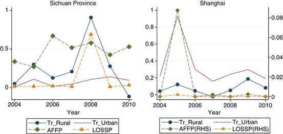

  

  Disaster damage and changes in transfers, Sichuan province and Shanghai.

• 3) Relief payments were not recorded separately at the central government level before 2010. Therefore, one is forced to rely on the times series for total transfers paid to residents.³⁰

Figure 1 is based on data from Sichuan Province and Shanghai city. The impact of the 2008 earthquake in Sichuan is clearly shown by the line labelled LOSSP on the left-hand side of Figure 1. Note that transfers to the urban population do not increase much in the wake of the earthquake, whereas transfers to the rural population exhibit a marked spike. This is consistent with the fact that farmers suffered more than urban citizens in such an agriculture-dominated province. By way of contrast, Shanghai is a city with few farmers and agricultural products. Transfers to urban residents in Shanghai are more sensitive to the impact of the powerful typhoon Matsa in 2005 as Figure 1 (RHS) shows. At the national level, however, rural residents are still the main victims of natural disasters to and income transferred to them is much less than urban citizens and more volatile (see Figure 2). This suggests that the relative change in total transfers paid to the rural population could be a more reliable proxy for the unobserved development of payments for disaster relief.

Figure 2

Disaster damage and average (change in) transfers to residents, whole China.

Two additional factors may affect the relative change in transfer payments: regional difference and the growth in agricultural subsidies. Table 6 reports the income transfers to three regions. While payments to eastern residents are almost two times as large as that of western and central ones, their rate of growth is the highest in the central part, with the western region ranking second.³¹ This calls for including regional dummy variables controlling for the increasingly preferential treatment of the central and western regions. Besides, Figure 2 indicates that the average growth rate of payments to rural residents is higher than that of payments to urban citizens, which likely reflects the agricultural subsidy policy started in early 2004. However, the growth in subsidies is relatively stable and can be controlled by adding a time trend in the empirical specification.

Table 6 Transfer payments to residents of three regions during 2004–2010 (in RMB per capita)

Other control variables

Other control variables include openness: total volume of exports and imports as a share of GDP; capital: gross capital formation as a share of GDP; and fdi: foreign direct investment as a share of GDP. These variables are frequently used in the literature on economic growth.³² The lagged terms of these variables are used in order to avoid simultaneity bias, since disasters may well affect their current values.

Empirical specification

The empirical model follows Noy2 by relating real per capita GDP growth to both the damage suffered from natural disasters and the amount of transfers paid for relief,

Here, y(i,t) denotes real GDP growth in region i in time t, with provincial GDP measured at constant prices, using the GDP deflator. This dependent variable is regressed on its lagged value y(i,t−1). In this way, region-specific influences that fail to be reflected in the fixed effect θ(i) are controlled for.³³ Also, recent research into the determinants of short- to medium-term growth suggests that the number of lags does not need to be extended beyond one year in annual data.³⁴ DM (disaster measure) is the relative importance of the damage caused by natural disasters as mentioned in the data section. The variable Tr is designed to reflect post-disaster transfers, calculated as the relative change in per capita transfers received by rural and urban households, divided by GDP deflator. The meaning of these two core variables is described in the data section above.

The interaction term DM × Tr is crucial for testing Proposition 2 because according to it, a given damage DM can have a different effect on economic growth depending on the extent to which transfers are paid (which are reflecting the loss in capital stock or loss in labour supply in the case of China). Here, the specification again follows Noy2 and McDermott.12

Finally, θ(i) represents the fixed effect pertaining to province i. Of course, there is no guarantee that unmeasured factors influencing θ(i) do not influence ɛ(it), the random error, as well. However, this risk is reduced by the inclusion of the lagged dependent variable, which picks up those unmeasured factors that are time-varying. t is the time trend as mentioned in data description section, controlling the time trend effect.

The coefficient β₂ pertaining to AFFP is expected to have a negative sign since natural disasters hurt labour supply, but it might also have a positive sign, being positively related to LOSSP to the extent that post-disaster investment might fully make up for the loss in capital. However, according to Proposition 2, the sign of β₃ should always be negative since transfers designed according to the loss in capital or labour are predicted to hamper economic growth more strongly when they increase in step with the size of the damage.

Estimation methodology

In view of the endogeneity introduced by the lagged dependent variable, Blundell-Bonds GMM estimation is applied. Blundell and Bond³⁵ combine Arellano and Bond's³⁶ difference GMM estimator with Arellano and Bover's³⁷ level GMM estimator. This approach significantly improves the efficiency of the two previous ones; however, it requires the lagged dependent variables after differentiation {Δy _i ,t−1, Δy _i ,t−2,…} to be uncorrelated with the random error term u _i ³⁸(pp. 179−181). However, Herzer et al.³⁹ point out that the GMM approach needs strong assumptions for consistent estimates and the weak instruments may bias coefficient estimates. Therefore, fixed effects regression is also employed as a check of robustness.⁴⁰ Robust standard errors are given in all the following regression reports in order to account for heteroscedasticity. The software used is STATA 10.0.

Regression results

Tables 7 and 8 relate real per capita income growth to the population affected and to direct economic losses incurred, respectively. Starting with Table 7, it may be noted that the coefficients of the lagged dependent variable have (highly significant) values between 0.39 and 0.44. After a shock, it therefore takes only between 1.64 and 1.79 years on average for a province to return to its long-term growth rate.

Table 7 Economic growth and share of population affected, system GMM estimator

Table 8 Economic growth and losses as a share of GDP, system GMM estimator

The four columns of Table 7 refer to different specifications. Column (1) abstracts from transfer incomes. The coefficient for AFFP says that a high share of population affected by natural disasters is strongly associated with a slower growth of real per capita GDP. An average disaster event (AFFP=0.33) would reduce growth contemporaneously by approximately 1.12 (=3.4 × 0.33) percentage points.

Column (2) introduces the two variables related to transfer, Tr_Rural and AFFP*Tr_Rural. While the (change in) transfers to rural households per se does not seem to have an impact on economic growth, the fact that it is geared to AFFP, the population affected, is seen to depress economic growth significantly, to the tune of some 6.85 percentage points per percentage point (change in) transfers, holding AFFP constant. This implies that at the mean values of about 0.33 for AFFP and 0.26 for Tr_Rural (see Table 2), disaster transfers to rural households are responsible for roughly 0.59 (=6.85 × 0.33 × 0.26) percentage points of growth loss. This does not seem much compared with the average growth rate of 12.8 per cent p.a.; however, there must be at least one instance where AFFP has reached its maximum value of 1.08 and Tr_Rural, its maximum value of 3.75 (both values reflecting the fact that a province can be hit by more than one disaster during a given year), while minimum average growth was as low as 5.4 per cent p.a. While this combination of values presumably does not apply to a single province, it does indicate that the effect of transfers on growth may be substantial in some cases.

In column (3) of Table 7, a test is performed by applying the specification of column (2) to the urban population. Since transfers paid to urban households are less sensitive to natural disasters (see the section “Data” above), the expectation is that they do not affect provincial economic growth significantly. This expectation is borne out in that AFFP is negatively related to growth as before, but the interaction variable AFFP × Tr_Urban is only significant at the 10 per cent level.

Finally, another specification test is performed in column (4) by using the (change in) total transfers as an explanatory variable. It is reassuring to see that while the other coefficients (among them, also the one pertaining to AFFP) are little affected, both Tr_All and AFFP*Tr_All are significant. In a less detailed analysis, one might have been tempted to conclude from the positive and significant coefficient of Tr_All that transfers possibly affect economic growth favourably. This shows the importance of distinguishing between relief payments going to rural and urban households when trying to discern their effects on economic growth. In sum, Table 7 provides clear empirical support for Proposition 2.

In Table 8, the same four specifications are displayed, but with AFFP replaced by the economic losses relative to GDP, LOSSP. It is gratifying to note that the coefficient of the lagged dependent variable implies an average adjustment period of 1.5 years, much the same as the values of Table 7.

Starting with specification (1), one recognises a (highly significant) negative effect of LOSSP on economic growth, amounting to an estimated 7.55 percentage points. To illustrate, let a province be hit by a disaster whose economic loss is the average of 2 per cent of its GDP (see Table 2). Ceteris paribus, one would predict its growth rate to drop by almost 0.15 (=7.55 × 0.02) percentage points. However, this estimate likely is on the high side because it is not replicated by the other specifications, where LOSSP never comes close to statistical significance.

Specification (2) again introduces an interaction term in the guise of LOSSP × Tr_Rural. Similar to the AFFP regression, the interaction term is negative and highly significant. More interestingly, the impact of LOSSP on growth turns out to be positive, though not quite significant. This might be consistent with the prediction of Proposition 1 that investment would increase after a disaster to compensate the loss of capital, boosting the economic growth. For an interpretation, let the growth of transferred income of rural household be the mean value of 0.26. A province with economic loss of 2 per cent of its GDP would tend to exhibit an increase in economic growth of 0.18 (=16.7 × 0.02–29.2 × 0.02 × 0.26) percentage points. However, the change in transfer payments still has a negative effect on growth by reducing the compensating investment.

Specification (3) in Table 8 again relates economic growth to the (change in) transfers paid to the urban population. As one would expect in view of the nature of these transfers (mainly pensions), these transfers do not contribute to economic growth, and there is no indication either of the interaction term LOSSP × Tr_Urban playing a role.

Column (4) of Table 8 contains a final specification check by again introducing the (change in) total transfers. The fact that LOSSP × Tr_All falls far short of statistical significance provides indirect corroborating evidence for the discussion in the section “Data”, which puts exclusive emphasis on the transfers paid to rural households.

The results displayed in Tables 7 and 8 may be summed up in two statements. First, the greater the share of the population affected by (and not necessarily the greater the economic loss suffered from) a natural disaster, the more important is the drop in the growth rates of Chinese provinces, ceteris paribus. Second, the faster the transfer payments increase as a signal of receiving disaster relief, the more they tend to stifle economic growth, likely through their depressing effect on the supply of labour and hence post-disaster investment.

Robustness checks

In this section, we present a range of robustness checks on the findings relating to the depressing effect of (the change in) transfer payments to rural residents.⁴¹ The findings suggest that the results reported in the previous section are quite robust to various changes in specification.

The disturbance of the year 2008

One concern with our results might be the potential disturbance of the year 2008, with its coincidence of the subprime mortgage crisis as well as the earthquake in Sichuan province. For this effect, we repeat the analysis by including a dummy for the year 2008 in Table 9 and excluding observations of this year in Table 10. The 2008 dummy variable in Table 9 is highly significant, suggesting that the subprime mortgage crisis led to a reduction by almost two percentage points in the growth rates of Chinese provinces. The coefficients of the interaction terms in the two tables are negative and significant in most cases. While the coefficients in Table 9 differ somewhat from the basic regressions, the estimation without the observations pertaining to the year 2008 is still consistent with the benchmark specification.

Table 9 Economic growth and disaster relief, including dummy for the year 2008

Table 10 Economic growth and disaster relief, with the year 2008 excluded

Including control variables

In Table 11 we present regression results including three growth-related factors as mentioned above. In addition, in order to control for the regional policy effects of transfer payments as discussed in the section “Data”, the variable Tr_Rural is interacted with the dummy for the western and central regions. As can be seen from Table 11, the coefficients of DM and DM × Tr_Rural are still consistent with the basic results. Note that the coefficients of openness, the share of total amount of imports plus exports in GDP, are negative and significant, which is quite counter-intuitive at first sight. However, a possible explanation is that in a first-order dynamic regression, reversion in a time series cannot be modelled directly. The variable openness might pick up this effect, since imports and exports typically decrease in the wake of a natural disaster which boosts transportation costs. This might be reasonable since we are running the regression in a dynamic structure and on the lagged term of openness, the negative sign might indicate the reversion behaviour in the time series. For the regional effect, the coefficients of Tr_Rural × West and Tr_Rural × Central imply that transfer payments to rural residents in the central and western regions are relatively higher than those going to the eastern part.

Table 11 Economic growth and disaster relief including control variables, GMM system estimator

Fixed effects regression

One might argue that the GMM approach could bias the estimation, since the instruments used might be weak while the assumptions for consistency are strong. In an attempt at avoiding these potential weaknesses of GMM estimation, we also present regression results using fixed effects regression (see Table 12). The lagged dependent variable is excluded to avoid an endogeneity problem. As can be seen from Table 12, the coefficients of the interaction term DM × Tr_Rural remain negative and significant. Most of the estimates are consistent with Table 11. Note that the effect of Tr_Rural on growth now becomes negative and significant, supporting the prediction of Proposition 1 that direct disaster relief has a negative impact on economic growth. However, the fixed effect model might fail to control for the time-variant region-specific influences as mentioned previously, and it might not be the appropriate methodology for empirical analysis in a dynamic structure.33

Table 12 Economic growth and disaster relief, fixed effects estimator

Binary measure of disaster relief

In Table 13 we present the regression results using a binary measure of disaster relief (=1 if Tr_Rural0.264, the mean value).⁴² As can be seen from Table 13, the major results reported previously are still robust. In columns (1) and (2) , the negative and significant coefficients of interaction term suggest that, for those provinces with Tr_Rural above mean value, the change in transfer payments aggravate the negative impact of AFFP by 1.36 percentage points. More interestingly, results in columns (3) and (4) indicate that LOSSP has a positive effect on economic growth only when provinces have a slower growth in Tr_Rural. For those provinces with Tr_Rural above average, LOSSP seems to hurt the economy by 9.41(=21.54–12.13) percentage points per one unit increase of LOSSP.

Table 13 Binary measure of disaster relief, system GMM estimator

Conclusion

The objective of this paper is to assess the impact of public relief on economic growth. A simple two-period model predicts that the substitution effect of disaster relief depresses labour supply, hampering post-disaster investment and hence economic growth. This prediction, formulated as Proposition 2, is tested using observations covering the 31 provinces and independent municipalities of China during 2004–2010. China provides an interesting test case because disaster relief is indeed paid according to the amount of disaster damage; moreover, it is reflected much more in the change in rural incomes than urban households, where pensions constitute the main component of public transfers.

The econometric inference combines level and change GMM estimation to deal with both endogeneity and heteroscedasticity. It produces a good deal of support for Proposition 2. First, disaster relief aggravates the negative impact of disaster damage measured by the population affected. Second, disaster relief impedes the possibly positive effect of disaster damage measured by direct economic losses.

These findings lend support to the policy advice based on Proposition 3 of Section “The Impact of Disaster Relief on Post-Disaster Investment”. It predicts that if transfers are conditioned on post-disaster labour supply rather than the loss of capital or labour endowment, the substitution effect of transfers can be alleviated by strengthening work incentives. One could cite the Chinese proverb, “If you give a man a fish, he will not go hungry for one day; if you teach him to fish, he will never go hungry again”. It appeals to the same logic as “food for work” in public welfare programmes. Public relief for disaster-stricken areas might take the form of investment in infrastructure and projects designed to prevent future disasters, both creating local employment. However, it could also take the form of assistance for finding employment in other areas of the country, not least by improving labour productivity through additional schooling and vocational training. In all, encouraging post-disaster labour supply is an important concern since it avoids the depressing effect of direct transfer payments.

Of course, this advice is based on an analysis that has its limitations. For one, the theoretical model may be too simplistic by neglecting problems of governance in the allocation of transfer relief. The fact that direct government assistance is often subject to corruption and the misappropriation of funds is an important aspect of the negative impact of transfer relief, which is not included in our model.⁴³ Second, the empirical evidence refers to China and may apply to other countries only with major modifications. Third, empirical testing has been hampered by data availability, the fact that the time series are fairly short, and disaster transfers were not measured directly. However, this work may still provide some preliminary insights into the adverse side effects of disaster relief and help redirect government intervention towards enhancing post-disaster labour supply.

Appendices

Appendix A

A1. Proof of Proposition 2

Proof: Given ΔTr=−δΔK₁, Eq. (9) shows that ΔI=−(1−δA₂) ΔK₁+A₁ΔH. Then we have ∂I/(−∂K₁)=1−δA₂<1. Post-disaster investment now does not fully compensate the loss in capital anymore. Similarly, when ΔTr=−δΔH, the change of investment is now ΔI=−ΔK₁+(A₁+δA₂)ΔH. Then ∂I/∂H=(A₁+δA₂)>A₁. Investment is now decreasing further. The reason is that one who suffers more is expected to receive larger transfer payments, and has less incentive to work in the second period. When labour supply declines, investment declines as well. In this case, direct disaster relief hinders post-disaster capital replacement and exaggerates the negative effect of labour loss. □

A2. Proof of Proposition 3

Proof: Since L₂ is an endogenous variable determined by the consumer, the first-order condition will be changed given that Tr=δL₂. The trade-off between second-period consumption and leisure is given by:

Using the Cobb-Douglas production function in Eq. (7), we can solve for the optimal investment in this case:

Then the marginal effect of Tr on investment can be easily obtained as follows⁴⁴:

Equation (A.2) shows that, given Tr=δL₂, the depressing effect of transfer payments on investment is now smaller. This is intuitive because the return of working now becomes higher with an extra income of transfer payments.

Appendix B

B1. The solution to Eqs. (1), (2), (3) and (4)

First, solve the following maximisation problem:

s.t.

Create a LaGrange function:

F.O.C

By solving the above-mentioned five first-order conditions the four equations (1), (2), (3) and (4) can be made available.

B2. Derivation of Eq. (9)

Eq. (6) substituted into Eq. (3) eliminates C2, and once that is substituted into the C–D production function (7) we get:

C–D function (7) substituted into Eq. (4) makes:

Simultaneously the above two equations create:

Substituting into the investment conditions (4) gives:

B3. The solution to Eqs. (11)–(12)

First, solve the following maximisation problem:

s.t.

Create a LaGrange function:

F.O.C

C-D function (7) substituted into above equations makes:

Combining with

We have

Since A₁=α(1−β)(βR)^1/(1−β)/(1−αβ), A₂=(1−α)βR/(1−αβ)

Substituting A1 and A2 into the above equation and we have

References

Anbarci, N., Escaleras, M. and Register, C.A. (2005) ‘Earthquake fatalities: The interaction of nature and political economy’, Journal of Public Economics 89 (9–10): 1907–1933.
Arellano, M. and Bond, S. (1991) ‘Some tests of specification for panel data: Monte Carlo evidence and an application to employment equations’, The Review of Economic Studies 58 (2): 277–297.
Arellano, M. and Bover, O. (1995) ‘Another look at the instrumental variable estimation of error-components models’, Journal of Econometrics 68 (1): 29–51.
Barry, F. (1999) ‘Government consumption and private investment in closed and open economies’, Journal of Macroeconomics 21 (1): 93–106.
Blundell, R. and Bond, S. (1998) ‘Initial conditions and moment restrictions in dynamic panel data models’, Journal of Econometrics 87 (1): 115–143.
Chang, K. (2010) ‘Community cohesion after a natural disaster: Insights from a Carlisle flood’, Disasters 34 (2): 289–302.
Chen, Q. (2010) Advanced Econometrics and the application of STATA, Beijing: Higher Education Press, pp. 179–181.
Hallegatte, S., Hourcade, J-C. and Dumas, P. (2007) ‘Why economic dynamics matter in assessing climate change damages: Illustration on extreme events’, Ecological Economics 62 (2): 330–340.
Han, L., Li, D., Moshirian, F. and Tian, Y. (2010) ‘Insurance development and economic growth’, The Geneva Papers on Risk and Insurance—Issues and Practice 35 (2): 183–199.
Herzer, D., Strulik, H. and Vollmer, S. (2012) ‘The long-run determinants of fertility: One century of demographic change 1900–1999’, Journal of Economic Growth 17 (4): 357–385.
Hirshleifer, J. (1966) ‘Disaster and recovery: The Black Death in Western Europe’, RAND Corporation Memorandum RM-4700-TAB, pp. 1–31.
Islam, N. (1995) ‘Growth empirics: A panel data approach’, The Quarterly Journal of Economics 110 (4): 1127–1170.
McDermott, T., Barry, F. and Tol, R. (2011) Disasters and development: Natural disasters, credit constraints and economic growth, ESRI Working Paper No 411.
National Bureau of Statistics of China (2012) China Statistical Yearbook 2012, Beijing: China Statistics Press.
Noy, I. (2009) ‘The macroeconomic consequences of disasters’, Journal of Development Economics 88 (2): 221–231.
Noy, I. and Vu, T.B. (2010) ‘The economics of natural disasters in a developing country: The case of Vietnam’, Journal of Asian Economics 21 (4): 345–354.
Raddatz, C. (2007) ‘Are external shocks responsible for the instability of output in low-income countries?’ Journal of Development Economics 84 (1): 155–187.
Rasmussen, T. (2004) Macroeconomic implications of natural disasters in the Caribbean, IMF Working Paper No. 04/224.
Skidmore, M. and Toya, H. (2002) ‘Do natural disasters promote long-run growth?’ Economic Inquiry 40 (4): 664–687.
Solow, R.M. (1956) ‘A contribution to the theory of economic growth’, The Quarterly Journal of Economics 70 (1): 65–94.
Toya, H. and Skidmore, M. (2007) ‘Economic development and the impacts of natural disasters’, Economics Letters 94 (1): 20–25.
Wang, Y., Chen, M. and Wang, X. (2008) ‘The impact of natural disasters on long-term economic growth’, Economics and Management 30 (19): 144–150.
Acknowledgements
We thank Peter Zweifel (University of Zurich) and Li Wang, Yu Shen and Jianpeng Zhang (Fudan University) for useful discussions. We also thank the anonymous reviewers for their valuable and constructive comments and suggestions to improve the paper. We gratefully acknowledge financial support from the 985 Project (2012SHKXQN006) and Shanghai Pujiang Program.
Author information
Authors and Affiliations