
Abstract
The paper presents a fault region identification method for the active distribution network (ADN) with limited PMU. First, PMU configuration and region division strategies are proposed based on the network topology. Next, the difference in three-phase current variations between the normal and fault regions of the ADN is analyzed. A multi-dimensional state monitoring matrix is built using the measured current data. The spectral norm ratio coefficient is constructed based on the 2-norm to lower the complexity of the multi-dimensional state monitoring matrix and quantify the difference in state changes before and after the fault occurs in each region. Then, the fault region is identified by combining each region’s spectral norm ratio coefficient and the change of the current phase. Finally, an IEEE 33-node simulation model is created to simulate faults under different working conditions. According to the simulation results, the suggested approach is less impacted by fault type, neutral point grounding mode, and transition resistance. Furthermore, even if the communication does not match the rigorous synchronization requirements, the proposed method can still complete the fault identification of the distribution network correctly and has high robustness.
Introduction
Active distribution network (ADN) is directly connected with users, which is the key link to ensure the quality of power supply and user service and improve the operation efficiency of power system. With the access of a large number of distributed energy resources such as photovoltaic solar, wind, and battery storage, the complexity of traditional fault location technology of single power system in active distribution network is also increasing. Therefore, it is urgent to propose an effective and fast fault location method for active distribution network.
The fault location methods of active distribution network are mainly based on electrical quantity, impedance, traveling wave method and intelligent algorithm. The method based on electrical quantities usually uses the positive sequence1,2 or zero sequence3,4,5 quantities during the fault to estimate the fault distance. However, too high transition resistance will make the change of electrical quantity not obvious, which will lead to the failure of location method. The impedance-based method mainly locates the fault by constructing the impedance matrix6,7,8. But the main flaw in the suggested techniques is that the impedance matrix construction cannot be done offline since the network structure changes due to sub-network formation and network reconfiguration. Thus, creating an impedance matrix does not significantly benefit large systems but increases complexity. The traveling wave method mainly uses the arrival time of the incident wave and the reflected wave to estimate the fault distance9,10. However, it must maintain the timing of measurements. What’s more, it requires high sampling frequencies and can be adversely affected by noise-corrupted measurements. The intelligent algorithm mainly uses the related optimization algorithm to realize the fault location. Refs.11,12,13 use Bayesian compressed sensing (BCS) to pinpoint all fault types in distribution networks. However, this method makes it easy to locate the adjacent regions of the fault region.
Phasor Measurement Units (PMUs) are being used increasingly often due to the ongoing advancements in communication technology, and they have grown to be a crucial component of the dynamic power system monitoring process. It obtains voltage and current phase data mainly by the discrete Fourier variation method. Based on the measurement data obtained by the PMU, it offers significant data support for the location of distribution network faults and effectively satisfies the demands for quick and precise fault location. Using the voltage threshold value determined by a thorough investigation of the test system, Reference14 uses the data from the optimal PMU locations to provide a two-stage fault detection method. However, does not specifically address how to get the optimal PMU location. Reference15 investigates a new field of study for defective region detection with little data from sensors in the power distribution system to address the issue of a large variety of PMU setups. In addition, literatures16,17,18 classify and locate the defects using deep learning algorithms based on measured data. The solutions, however, will not operate in a distribution network system with DGs and are only helpful for traditional distribution networks.
This paper analyzed the fault characteristics in ADN. Based on the characteristics of current variation before and after the fault occurs, the spectral norm ratio coefficient (SNRC) and current phase difference (CPD) are defined. The proposed method only needs current amplitude and phase data of any period before and after the fault occurs, so it can avoid the impact of time synchronization on fault region identification. Moreover, the method is not affected by fault type, neutral point grounding type, and transition resistance.
The remaining of this article is as follows: “Fault features of active distribution network” section analyzes current features in ADN. How to implement fault region identification using the SNRC and CPD is described in “Fault region identification method” section. “Simulation results” section uses PSCAD and MATLAB to verify the effectiveness of the proposed method from different fault position, fault types, neutral point grounding methods, and transition resistances. “Experiment results” section verifies the practical significance of the method. The conclusion is presented in “Conclusion” section.
Fault features of active distribution network
Fault features of distribution network without DG
Figure 1 illustrates this by using the A-phase ground fault at fault point F as an example (for research, L1 and L2 are set as the upstream and downstream lines of point F, respectively). The present relationship between lines L1, L2, and L3 is satisfied after the fault occurs as follows:
where I1AF, I1BF, and I1CF are the A, B, and C three-phase currents of line L1, respectively. IfA, IfB, and IfC are the fault currents of the A, B, and C phases at the fault point F, respectively. VfA, VfB, and VfC are the fault voltages of A, B, and C phases at the fault point F, respectively. Zd is the sum of Z2 and Z3.

Distribution network without DG.
When an A-phase grounding fault occurs, there are:
where Vf(0) is the voltage before fault at fault point F and a is equal to ej120. Z(1) is the sum of equivalent positive sequence impedance in line, Z(2) is the sum of equal negative sequence impedance in line, and Z(0) is the sum of equivalent zero sequence impedance in line. In this paper, Z(1) equals Z(2).
Combined with Eqs. (1)-(2), the currents of L1A, L1B, and L1C after fault are:
The currents of line L2 and L3 after the A-phase fault are:
Thus, the current variation of L1B, L1C, L2, and L3 are:
In the formula, VfB(0) and VfC(0) are the voltages of the B and C phases before fault at fault point F.
The current variation of lines L1A is:
According to Eqs. (5), (6), the sum of the fault current and the phase current downstream of the fault site is the fault phase current upstream of the fault point.
When a B and C two-phase ground short circuit occurs at point F, the current of line L1 may be determined as follows:
where, I1AF, I 1BF, and I1CF are the A, B, and C three-phase currents of line L1, respectively. IfB and IfC are the fault currents of the B and C phase at the fault point F, respectively. VfA, VfB, and VfC are the fault voltages of A, B, and C phases at the fault point F, respectively. Zd is the equivalent impedance from fault point F to the end of the line.
When a BC two-phase ground short circuit occurs in the distribution network, there are:
where IfB and IfC are the fault currents of B and C phases at fault point F. VfA, VfB, and VC are the fault voltages of the A, B, and C phases at fault point F. IfA(1) is the positive sequence current of the A phase in line L1 and a is equal to ej120, Vf(0) is the voltage before fault at fault point F. Z(1) is the sum of equivalent positive sequence impedance in line, Z(2) is the sum of equal negative sequence impedance in line, and Z(0) is the sum of equivalent zero sequence impedance in line. ZP is the parallel equivalent resistance of Z(2) and Z(0). In this paper, Z(1) equals Z(2).
Combined with Eqs. (7)-(8), the currents of L1A, L1B, and L1C after fault are:
The currents of line L2 and L3 after the B, and C two-phase ground fault are:
Therefore, the current variation of L1A, L2, and L3 is:
where, VfB(0) and VfC(0) are the voltages of the B and C phases before fault at fault point F.
The current variation of lines L1B and L1C is:
Equations (10)-(12) demonstrate that when a two-phase fault occurs, the current of the fault phase downstream of the fault point is zero. The sum of the fault current and the phase current downstream of the fault point is the fault phase current upstream of the fault point. Because the voltage at the fault point is zero when a three-phase short-circuit fault occurs, the current downstream of the fault point is also zero. The current of the fault phase downstream of the fault point decreases when a phase-to-phase short-circuit fault occurs, and the mechanism is identical to a two-phase short-circuit fault. This paper will not be duplicated due to space limitations. In summary, when a fault occurs, the current of the fault phase upstream of the fault point is greater than the current of the fault phase downstream of the fault point.
Fault features of distribution network with DG
For the fault features of the downstream region without DG (i.e., the Region 2 in the Fig. 2), as shown in Fig. 2, when a fault occurs, the system power supply and DG will both provide a short-circuit current to the fault point.

Distribution network with DG.
Assuming that the positive direction is the direction of current flow out of the bus. At this time, the current variations of nodes Q and J before and after faults are:
where, Δis is the current variation the system power supply provides before and after the fault. Δidg is the variation provided by DG, and iJ is the current at point J before the fault.
When a fault occurs in the Region 2, i.e., fault f3, the current variation downstream of the fault point equals the current before the fault, and the current variation upstream of the fault point equals the sum of the system power supply current variation and the current variation supplied by the DG. So, by contrasting the current amplitude difference before and after the fault, the fault region may be identified.
For the fault features of the downstream region with DG (i.e., the Region 1 in the Fig. 2), as shown in Fig. 2, when a fault occurs, the fault current from DG will flow to the fault point if DG is connected to the fault region. Point M of the Region 1 in Fig. 2 is arbitrarily chosen to study the current attributes of the upstream and downstream fault. The direction of the current flowing out of the bus is the positive direction.
When no fault occurs, the current IMpre of the point M is:
VS and VM are the system source and M-point voltage during the regular line operation. ZT is the sum of the internal impedance of the transformer and the system source. Z1 and Z2 are the line impedances.
-
1.
Single-phase fault feature in Region 1 of Fig. 2.
Suppose that an A-phase fault occurs upstream of the detection point M, as shown in f1 of Fig. 2. The current IMF1 of the point M is:
$$I_{{{\text{MF1}}}} = \frac{{V_{f1} - V_{Q} }}{{Z_{{2}} + Z_{3} + Z_{4} }}$$(16)where Vf1 and VQ are the fault point’s and Q point’s voltage, respectively. Z2, Z3, and Z4 are the line impedances.
If the transition resistance is 0, it is obvious to find:
$$\left\{ \begin{aligned} & V_{f1} = 0 \hfill \\ & I_{{{\text{MF1}}}} = \frac{{ - V_{Q} }}{{Z_{{2}} + Z_{3} + Z_{4} }} \hfill \\ \end{aligned} \right.$$(17)Hence, IMF1 is negative. the length of the line is generally not more than a few kilometers when the distribution network is operating normally, and the length of the line less impacts the impedance angle. It can be considered that the line impedance angle is roughly equal, ranging from 70° to 80°19. As a result, in Eq. (15), the amplitude of VS-VM is lower, and the phase is earlier than VS. Transformer impedance and system impedance are both contained in ZT. Its maximum impedance angle is not more than 90°, so the phase of IMF1 lies behind the phase of IMpre. If there is a transition resistance since the amplitude of the DG access point voltage is greater than Vf1, Vf1-VQ is negative, and the phase of IMF1 still lags behind the phase of IMpre.
Assume that an A-phase fault develops downstream of point M, as shown in f2 of Fig. 2. The current IMF2 of the point M is:
$$I_{{{\text{MF2}}}} = \frac{{V_{{\text{S}}} - V_{f2} }}{{Z_{{\text{T}}} + Z_{1} + Z_{2} + Z{}_{3}}}$$(18)where Vf2 and VS are the fault point and system source voltage, respectively. Z1, Z2, and Z3 are the line impedances. ZT is the sum of the internal impedance of the system source and the impedance of the transformer.
According to the study above, the phase of IMF2 is ahead of the phase of IMpre if the transition resistance is 0. On the other hand, the phase of Vf2 is behind the phase of the f2-point voltage when the line is operating normally. As a result, the phase of Vf2 is later than the phases of VM and VS. It can be determined that the phase of IMF2 is ahead of the phase of IMpre.
-
2.
Two-phase short fault and three-phase short fault feature in Region 1 of Fig. 2.
When a two-phase short-circuit fault occurs, the voltage phase of the access point will mutate. As a result, it is appropriate to use positive sequence quantity for analysis. Suppose that a BC two-phase short-circuit fault occurs upstream of point M, as illustrated in f1 of Fig. 2, and that the phase of the A-phase voltage at fault time is 0 degree as a reference. Figure 3 depicts the equivalent circuit at f1 fault.
Figure 3 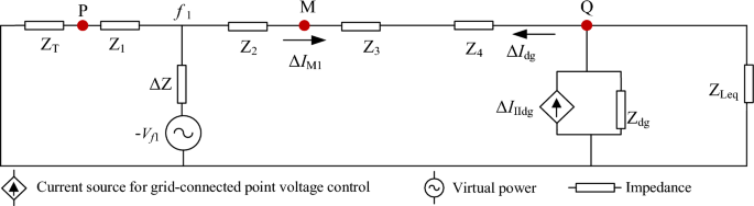
Equivalent circuit at f1 fault.
The positive sequence current variation ΔIM1 of M point is:
$$\Delta I_{{{\text{M1}}}} = - \Delta I_{dg}$$(19)where, ΔIdg is the variation of the output current of DG. When the inverter-type DG output current is equal to 1.2 p.u., the amplitude range of the positive sequence fault component before and after the M-point fault is obtained as follows:
$$|\Delta I_{{{\text{dg}}}} | \in 0.22p.u.\sim 0.61p.u.$$(20)ΔIM1 is negative, so the current of M point phase lags behind IMpre phase after a fault. Assume that a BC two-phase short-circuit fault occurs downstream of point M, as depicted in f2 of Fig. 2. The equivalent circuit at f2 fault is shown in Fig. 4.
Figure 4 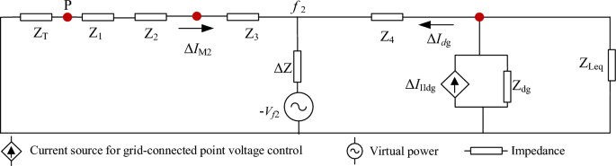
Equivalent circuit at f2 fault.
According to the superposition theorem, the current positive sequence variation ΔIM2 of M can be obtained as:
$$\begin{aligned} \Delta I_{{{\text{M2}}}} & = \frac{{V_{f2} }}{{\Delta Z + (Z_{T} + Z_{1} + Z_{2} + Z_{3} )||(Z_{4} + (Z_{{{\text{Leq}}}} ||Z_{dg} )}} \cdot \frac{{(Z_{4} + (Z_{{{\text{Leq}}}} ||Z_{dg} )}}{{Z_{T} + Z_{1} + Z_{2} + Z_{3} + Z_{4} + Z_{{{\text{Leq}}}} + Z_{dg} }} \hfill \\ & \quad - \Delta I_{dg} \cdot \frac{\Delta Z}{{\Delta Z + (Z_{T} + Z_{1} + Z_{2} + Z_{3} )}} \hfill \\ \end{aligned}$$(21)where Zdg is the internal impedance of DG and ZLeq is the sum of the impedance downstream of the Region 1 and the load. ΔZ is the transition resistance. “||” is the parallel operation of impedance. For the virtual power branch, because the internal impedance of the inverter-type DG is infinite, it can be simplified as follows:
$$\begin{aligned} \Delta I_{{{\text{M2}}}} & = \frac{{V_{f2} }}{{\Delta Z + (Z_{T} + Z_{1} + Z_{2} + Z_{3} )}} - \Delta I_{dg} \cdot \frac{\Delta Z}{{\Delta Z + (Z_{T} + Z_{1} + Z_{2} + Z_{3} )}} \hfill \\ & = \frac{{V_{f} - \Delta I_{dg} \Delta Z}}{{\Delta Z + (Z_{T} + Z_{1} + Z_{2} + Z_{3} )}} \hfill \\ \end{aligned}$$(22)When a fault occurs, the amplitude of the positive-sequence voltage at the fault point is half what it was before the fault, and the voltage phase stays unaltered. The amplitude of the positive-sequence fault component of the virtual power supply's current is 3 to 12 times that of the DG's current. When the inverter-like DG’s output current is set at 1.2 p.u., according to reference19, there is:
$$\left\{ \begin{aligned} & |\Delta I_{{{\text{M2}}}} | \in 2.86p.u.\sim 11.94p.u. \hfill \\ & |\Delta I_{{{\text{dg}}}} | \in 0.22p.u.\sim 0.61p.u. \hfill \\ \end{aligned} \right.$$(23)Therefore, the direction of ΔIM2 is positive, implying that the current phase of M point is ahead of the phase of IMpre after the fault. Taking the impedance angle of the overhead line as 72°19, the phase angle variation of the positive sequence fault component at both ends of the Region 1 may be calculated roughly as:
$$\arg (\Delta I_{PQ} ) \in (0^{ \circ } ,87.3^{ \circ } )$$(24)If a three-phase short-circuit fault occurs upstream and downstream of point M, it is seemingly possible to find:
$$\left\{ \begin{aligned} & |\Delta I_{{{\text{M1}}}} | = |\Delta I_{{{\text{dg}}}} | \in 0.22pu\sim 2.0pu \hfill \\ & |\Delta I_{{{\text{M2}}}} | \in 5.58pu\sim 12.44pu \hfill \\ \end{aligned} \right.$$(25)where |ΔIM1| is M point upstream fault current amplitude variation. |ΔIM2| is M point downstream fault current amplitude variation.
Combining Eqs. (19), (22), and (25), it can be obtained that the phase of ΔIM1 is behind the phase of IMpre, whereas the phase of ΔIM2 is ahead of the phase of IMpre. Therefore, the phase angle variation of the positive sequence fault component at both ends of the Region 1 can be approximated as follows:
$$\arg (\Delta I_{PQ} ) \in (0^{ \circ } ,162.9^{ \circ } )$$(26)From above, when a fault occurs in a downstream region with DG access, the positive sequence fault current phase upstream of the fault point will be ahead of the normal operation phase. In contrast, the positive sequence fault current phase downstream of the fault point will lag. If we define φp as the phase before the fault and φF as the phase after the fault, then the phase variation ∆φ is:
$$\Delta \varphi = \varphi_{{\text{p}}} - \varphi_{{\text{F}}}$$(27)If ∆φ is positive, the phase after the fault is ahead of the phase before the fault. If ∆φ is negative, the phase after the fault lags behind the phase before the fault.
When a fault occurs in the Region 2 in Fig. 2, there is IPF = IQF. At both ends of the Region 1, the CPD of the positive fault sequence current is:
$$\Delta \varphi_{PQ} = |\Delta \varphi_{P} - \Delta \varphi_{Q} | = 0$$(28)The above analysis shows that the fault positive sequence current phase at upstream of the fault point is ahead of the phase before the fault. In contrast, the fault positive sequence current phase at downstream of the fault point lags behind the phase before the fault, resulting in the maximum amount of phase difference in faulty region. Equations (24) and (26) illustrate the range.


Fault region identification method
Spectral norm ratio coefficient
The matrix 2-norm of the factual matrix Am×n is defined as follows:
where A is an m × n matrix, AT is a transposed matrix of A. eig(.) is the eigenvalue calculation function of a square matrix. eig (AT × A) represents the eigenvector [λ1, …, λi, …]T of matrix A. λi represents the ith eigenvalue.
In this research, the length of the data acquisition time window is set to 10 ms. A fault is considered to have occurred when the current data acquired by the PMU exceeds the threshold. Data from each cycle before the fault is collected and discretized. The phase current matrix of node i before the fault is:
where i = 1, 2, 3, …, N; k = 1, 2, 3, …, M. IiA(k), IiB(k), IiC(k) are the current amplitudes of the kth sampling point of the node I before the fault occurs, and M is the total number of data obtained by discretization.
After a length of time, the current IiF of each node is derived using discretization:
where i = 1, 2, 3, …, N; k = 1, 2, 3, …, M. I iFA(k), IiFB(k), IiFC(k) are the current amplitudes of the kth sampling point of the node i after the fault.
To realize fault region identification under limited PMU, the SNRC is defined to measure the difference between the upstream and downstream currents of the fault point. The expression of SNRC is as follows:
where, ||Ii||2 represents the 2-norm of the current before the fault of node i, and ||IiF||2 represents the 2-norm of the current after the fault of node i. Then the SNRC variation ΔKm of the region m (the first node and end node of region m are nodes i and j, respectively) is:
where m = 1, 2, 3, …, J; i, j = 1, 2, 3, …, N, and i ≠ j.
When the line is in normal operation, the 2-norm of the three-phase current calculated for the entire line for any period is not significantly different. Hence, the ΔK of each region is close to 0. When the line faults, the phase current is greater than the threshold Iset, and the ΔK of each region increases. Moreover, the ΔK of the fault region is significantly greater than the ΔK of the normal region. As a result, the fault region may be identified by comparing the variations in ΔK of each location.
Current phase angle difference
Because there is no current flowing downstream of the fault point when a fault occurs in the downstream region without DG integration, the fault region may still be recognized using the SNRC. When a fault occurs in the downstream region with DG access, the DG injects current into the fault point. Current flows downstream of the fault point. Relying exclusively on the SNRC may lead to errors. Equations (26)–(28) shows that the CPD of the normal region is 0. However, the CPD of the fault region will be much more significant than that in the normal region. To identify the fault region, this study combines the CPD stated in Eq. (34) with the SNRC.
where φMF and φNF are the current phases after node M and N fault, respectively. φM and φNP are the current phases before node M and N fault, respectively. ΔφM is the current phase variation of node M. ΔφN is the current phase variation of node N. ΔφMN is the CPD of the region (node M and node N are the first node and end node of the region, respectively.) If the region MN is normal, then its ΔφMN approaches 0. Inversely, its ΔφMN will be the maximum one.
Fault region identification start criterion
In this paper, PMUs are utilized to monitor the phase current in real-time. Meanwhile, the exists of faults is determined based on whether the phase current exceeds the limit. The particular requirement is as follows:
where Iset is the fault protection threshold. The neutral point ungrounded system threshold Iset-U and the neutral point through the arc suppression coil grounding system threshold Iset-A respectively, meet:
where, Krel is the reliability coefficient, generally 0.8; ICΣ is the total ground capacitive current; IL is the maximum line-to-ground capacitance current; and W is the over-compensation degree.
When the above starting criterion is satisfied at time t, PMU will take the point at time t as the fault starting point and record the phase current data before the fault starting point and the phase current data of a cycle after the fault starting point. According to the data, the PMUs at both ends of the region use Eqs. (32)–(34) to identify the fault region.
To eliminate the impact of other interference signals on the beginning fault region identification, the PMU is utilized to capture phase current data one cycle after the fault starting point for verification after finding the fault starting point. If Eq. (37) is fulfilled, the identification and the next step are determined.
where, Ikm is the practical phase current value in one cycle, and K is the reliability coefficient of phase current fault, generally K = 2–3. In is the reasonable value of phase current when the line is normal, and in(k) is the instantaneous value of phase current at the kth identification point after the fault.
PMU configuration and region division strategies
The PMU configuration and region division strategies are proposed in this paper, as shown in Fig. 5. Specifically, the PMU configuration strategy is as follows:
-
1.
The first node of main feeder and the end node of main feeder in ADN are arranged with PMU, respectively;
-
2.
The first node of branch and the end node of branch are arranged with PMU, respectively.

Diagram of PMU configuration and region division.
In addition, the region division strategy is:
-
1.
The first node of main feeder and the first node of the nearest brunch in distribution network is the regional boundaries;
-
2.
The first node of branch and the end node of the branch is the regional boundary;
-
3.
The end node of main feeder and the first node of the nearest branch is the regional boundaries.
Fault region identification method steps
The framework and flowchart of the proposed method shown in Figs. 6-7. The implementation steps are as follows:

The framework of the proposed method.

The flowchart of the proposed method.
- Step 1::
-
arrange the PMUs according to the proposed method and divide the region.
- Step 2::
-
use the three-phase current data collected by PMUs. Judge the fault according to Eqs. (35)–(37).
- Step 3::
-
calculate and compare ΔKj of each region based on Eqs. (29)–(33) to gain the region corresponding to the ΔKmax.
- Step 4::
-
calculate and compare Δφj of each region based on Eq. (34).
- Step 5::
-
if the region corresponding to ΔKmax is the same as that corresponding to ∆φmax, output the region name. Adversely, output the region corresponding to ∆φmax.
Simulation results
The IEEE 33-node system is built in PSCAD/EMTDC, using a simulation sampling frequency of 4 kHz. The parameters of the system are shown in the Supplementary Information. The capacities of DG1 and DG2 are 0.544 MVA and 1.4 MVA, respectively. MatlabR2016b is utilized for data analysis and computation to verify the effectiveness of the proposed fault region identification method. According to the method of PMU layout and region division, the nodes and region division of PMU in an IEEE 33-node distribution network are shown in Fig. 8.

IEEE 33-node distribution network.
Firstly, set an A-phase grounding fault in Region 7 and combine it with the phase current data collected by PMU. The curve of ΔK variation with time in each region is obtained, as depicted in Fig. 9(a). Secondly, set up a phase A grounding fault in Region 2 and use the data collected by PMU. The ΔK variation and CPD with time in each region is obtained, as shown in Fig. 9(b)-(c).

ΔK and Δφ in each region in case of fault in Region 7 and Region 5 respectively. (a) ΔK for each region in case of fault in Region 7; (b) ΔK for each region in case of fault in Region 5; (c) Δφ for each region in case of fault in Region 5.
Figure 9(a) shows that the ΔKmax occurs when a fault occurs in a region without DG access downstream. Additionally, Fig. 9(b)-(c) show that when a fault occurs in a region with DG access downstream, its ΔK is second only to ΔKmax, but the CPD is at its maximum. To accurately identify the fault region, the SNRC and CPD of the region can be combined.
To verify the reliability and robustness of the method, the fault type, neutral point grounding mode, and fault transition resistance of the line are changed, respectively. The results are illustrated in Figs. 10-11 and Tables 1-2. From the results in Fig. 10, the SNRC variation and CPD of Region 2 reach their maximum when two-phase faults and three-phase faults occur in Region 2. This is because the short-circuit current delivered by DG1 and DG2 is slight when a two-phase or three-phase fault occurs.

Identification results under different fault types in Region 2. (a) Single-phase fault; (b) Two-phase fault; (c) Three-phase fault.

Identification results of Region 2 fault under different neutral grounding modes. (a) Neutral point ungrounded mode; (b) Neutral point through low resistance grounding mode; (c) Neutral point grounding through arc suppression coil.
Figure 11 shows the identification results under various neutral point grounding modes, indicating that the grounding mode of the neutral point has little effect on the proposed method and that the fault region can still be accurately identified under various neutral grounding modes.
The results and analyses in Tables 1-2 reveal that the method has a decent identification impact in any location. The smaller the ΔK and Δφ of each region, the more excellent the transition resistance. Furthermore, the SNRC variation of the fault region will reach their maximum values. This is because the short-circuit current of the distributed power supply is reduced when the transition resistance increases. As a result, in the case of a high impedance fault, the method proposed can still identify the fault region.
Table 3 demonstrates the identification result with the PMU installed in node 2 takes 10 ms longer to gather data than other PMUs. It can be obtained that when a single-phase ground fault occurs in Region 7, the ΔK and Δφ of Region 7 are greater than those in other regions. While a single-phase ground fault occurs in Region 2, the Δφ of Region 2 reaches the maximum. And the ΔK of Region 2 is the second largest compared with other regions. This is because the estimated current spectrum norm measures the current's variation in a data window, whereas the current phase utilizes the steady-state value. As a result, the method suggested in this research has low communication needs between PMUs.
In order to verify the effectiveness of the proposed method in large-scale distribution networks, this paper builds an IEEE 69-node distribution network system as shown in Fig. 12. The parameters of the system are shown in the Supplementary Information. The capacities of DG1 and DG2 are 0.544 MVA and 1.4 MVA, respectively. Set an A-phase grounded fault in R7(node 12-node 27) and R8(node 3-node 69), respectively. Collect the current data of each cycle before and after the fault to calculate the ΔK of each region. The result is shown in Table 4. It can be obtained that when a fault occurs in the region downstream of the fault point accessing the DG (e.g., R7), the Δφ of the fault region are significantly larger than those of the other regions. And the ΔK will reach the maximum or the second largest. When a fault occurs in the region downstream of the fault point without access to the DG (e.g., R8), the ΔK and Δφ in the fault region are both significantly larger than those in normal regions. Therefore, the method proposed in this paper is still able to effectively and accurately identify fault region under large-scale distribution networks.

IEEE 69-node distribution network.
To further verify the superiority of the methods proposed, this paper compared it with other four methods. The four methods use the characteristics of the upstream and downstream currents at the fault point to realize fault identification. Reference20 realizes fault region identification with the help of zero sequence conductance. Although it is independent of neutral grounding method, transition resistance and communication desynchronization, it can only identify single-phase faults and can only be applied to single-supply systems. Literature21, compared to literature20, is independent of fault type, but it requires communication synchronization. The methods proposed in literatures22,23 are applicable to DG-integrated distribution networks, but do not consider the effects of neutral grounding method, transition resistance and communication desynchronization. The specific method comparison results are shown in Table 5. Therefore, method proposed in this paper is more comprehensively considered and superior to other methods.
Experiment results
To verify the efficacy and dependability of the proposed method, a real 6-node test platform is used to validate the method. Figure 13 depicts the test platform structure, PMU configuration, and region division. The power quality analyzer replaces the PMU in the actual test, and three power quality analyzers acquire the platform’s current data before and after the short-circuit defect at a 4 kHz acquisition frequency. Simultaneously, a sampling time of 10 ms is set between the three power quality analyzers mentioned above to examine the proposed method's performance change when the PMU clock is not synced.

Test platform (a) The topology of the test platform; (b) The actual test platform.
In the actual experiment, the fault is set in Region 1 and Region 2, respectively. Figure 14 depicts the measured waveforms of the currents at both ends of the region when Region 1 and Region 2 fault respectively. It can be found that when Region 1 faults, the current at node 1 increases and the currents at node 3 and node 6 remain essentially unchanged. Whereas, when Region 2 faults, the currents at both node 1 and node 2 increase and the current at node 6 remains essentially unchanged. The fault region identification results obtained by the proposed method are shown in Table 6. It can be obtained that the ΔK and Δφ of the faulty region are significantly larger than those of the normal region when either Region 1 or Region 2 fault. Thus, the method proposed in this paper can still accurately identify the fault region when the communication is not synchronized, proving its practical potential.

Measured current waveform of each node (a) Region 1 faults; (b) Region 2 faults.
Conclusion
The paper analyzes the fault characteristics of the ADN in detail. A fault region identification approach based on the SNRC and CPD is proposed for the ADN. It only needs to extract the current amplitude and phase data of any period before and after the fault occurs, avoiding the impact of time synchronization on fault region identification. Case studies of faults under different conditions are used to evaluate the performance of the proposed method. The results demonstrate that the method is less affected by fault type, neutral grounding mode, fault position, transition resistance, and communication. Moreover, the actual test platform shows that the proposed method can effectively identify the fault region and has practical significance.
With the further development of synchronous measuring technology, PMU will become more commonly employed in distribution networks. Understanding how to use restricted PMU to accomplish accurate fault location in the ADN is critical.
Data availability
The datasets used and/or analyzed during the current study available from the corresponding author on reasonable request.
References
Barik, M. A. et al. A decentralized fault detection technique for detecting single phase to ground faults in power distribution systems with resonant grounding. IEEE Trans. Power Deliv. 33, 2462–2473. https://doi.org/10.1109/TPWRD.2018.2799181 (2018).
Liao, F., Li, H. & Chen, J. High-impedance ground fault detection based on phase current increment ratio. In 2019 IEEE 8th International Conference on Advanced Power System Automation and Protection (APAP), 841–845 https://doi.org/10.1109/APAP47170.2019.9224929 (2019).
Fen, G. et al. Faulted line detection using time-frequency information for distribution system. In 2020 IEEE/IAS Industrial and Commercial Power System Asia (I&CPS Asia), 976–981 https://doi.org/10.1109/ICPSAsia48933.2020.9208520 (2020).
Liang, H., Li, H. & Wang, G. A single-phase-to-ground fault detection method based on the ratio fluctuation coefficient of the zero-sequence current and voltage differential in a distribution network. IEEE Access 11, 7297–7308. https://doi.org/10.1109/ACCESS.2023.3238072 (2023).
Li, L., Gao, H., Cong, W. & Yuan, T. Location method of single line-to-ground faults in low-resistance grounded distribution networks based on ratio of zero-sequence admittance. Int. J. Electr. Power Energy Syst. https://doi.org/10.1016/j.ijepes.2022.108777 (2023).
Galvez, C. & Abur, A. Fault location in active distribution networks containing distributed energy resources (DERs). IEEE Trans. Power Deliv. 36, 3128–3139. https://doi.org/10.1109/TPWRD.2020.3034179 (2021).
Buzo, R. F., Barradas, H. M. & Leão, F. B. A new method for fault location in distribution networks based on voltage sag measurements. IEEE Trans. Power Deliv. 36, 651–662. https://doi.org/10.1109/TPWRD.2020.2987892 (2021).
Mirshekal, H. et al. A novel fault location methodology for smart distribution networks. IEEE Trans. Smart Grid 12, 1277–1288. https://doi.org/10.1109/TSG.2020.3031400 (2021).
Shunhu, D. et al. Travelling wave signal processing method based on fruit fly algorithm and stochastic resonance. In 2021 IEEE Sustainable Power and Energy Conference (iSPEC), 4069–4073 https://doi.org/10.1109/iSPEC53008.2021.9736058 (2021).
Huo, W. et al. Fault location of cable hybrid transmission lines based on energy attenuation characteristics of traveling waves. Sci. Rep. 12, 22448. https://doi.org/10.1038/s41598-022-25976-8 (2022).
Majidi, M., Arabali, A. & Etezadi-Amoli, M. Fault location in distribution networks by compressive sensing. IEEE Trans. Power Deliv. 30, 1761–1769. https://doi.org/10.1109/TPWRD.2014.2357780 (2015).
Majidi, M. & Etezadi-Amoli, M. A new fault location technique in smart distribution networks using synchronized/nonsynchronized measurements. IEEE Trans. Power Deliv. 33, 1358–1368. https://doi.org/10.1109/TPWRD.2017.2787131 (2018).
Jiang, K. et al. Block-sparse Bayesian learning method for fault location in active distribution networks with limited synchronized measurements. IEEE Trans. Power Syst. 36, 3189–3203. https://doi.org/10.1109/TPWRS.2021.3049443 (2021).
Das, D., Maji, S. & Kayal, P. Detection of faulty regions in power distribution grid with limited measurement. In 2021 IEEE 2nd International Conference on Electrical Power and Energy Systems (ICEPES), 1–5 https://doi.org/10.1109/ICEPES52894.2021.9699580 (2021).
Jain, A., Archana, T. C. & Sahoo, M. B. K. A methodology for fault detection and classification using PMU measurements. In 2018 20th National Power Systems Conference (NPSC), 1–6 https://doi.org/10.1109/NPSC.2018.8771757 (2018).
Zhao, M. & Barati, M. A real-time fault localization in power distribution grid for wildfire detection through deep convolutional neural networks. IEEE Trans. Ind. Appl. 57, 4316–4326. https://doi.org/10.1109/TIA.2021.3083645 (2021).
Du, Y. et al. Single Line-to-ground faulted line detection of distribution systems with resonant grounding based on feature fusion framework. In 2020 IEEE Power & Energy Society General Meeting (PESGM), 1–1 https://doi.org/10.1109/PESGM41954.2020.9281661 (2020)
Hu, C., Qu, N. & Zhang, S. Series arc fault detection based on continuous wavelet transform and DRSN-CW with limited source data. Sci. Rep. 12, 12809. https://doi.org/10.1038/s41598-022-17235-7 (2022).
Gao, H., Li, J. & Xu, B. Principle and implementation of current differential protection in distribution networks with high penetration of DGs. IEEE Trans. Power Deliv. 32, 565–574. https://doi.org/10.1109/TPWRD.2016.2628777 (2017).
Li, L., Gao, H., Cong, W. & Yuan, T. Location method of single line-to-ground faults in low-resistance grounded distribution networks based on ratio of zero-sequence admittance. Int. J. Electr. Power Energy Syst. 102, 11–12 (2018).
Zhang, B., Liu, H., Song, J. & Zhang, J. Simulation on grounding fault location of distribution network based on regional parameters. In 2019 IEEE 19th International Symposium on High Assurance Systems Engineering (HASE), 216–221 (2019).
Ganivada, P. K. & Jena, P. A fault location identification technique for active distribution system. IEEE Trans. Ind. Inform. 18(5), 3000–3010 (2022).
Zhang, C., Liu, Z., Huang, J., Wang, B. & Wang, X. Fault location in active distribution network based on the change of current phase. In 2017 IEEE Conference on Energy Internet and Energy System Integration (EI2), 1–5 (2017).
Acknowledgements
This work was supported in part by the Science and Technology Projects of China Southern Power Grid, Co., Ltd. (Grant No. GDKJXM20231017), in part by Shenzhen Science and Technology R&D Fund for undertaking Major National Science and Technology Project of China (Grant No. CJGJZD20200617102405015), and in part by the International Science and Technology Cooperation Program of China (Grant No. 2022YFE0129300).
Author information
Authors and Affiliations
Contributions
J.C. contributed to conceptualization, formal analysis, design methodology, writing the original draft. Y.L. contributed to resources, supervision, validation, project management, and intellectual content revising. R.Z. contributed supervision, revising and language editing for intellectual content. JL.L. contributed resources and supervision. A.C. contributed to data reduction and project administration. L.H. contributed to project administration. L.Z. contributed to data curation and source code checking. M.S. contributed to project administration. All authors reviewed the manuscript.
Corresponding authors
Ethics declarations
Competing interests
The authors declare no competing interests.
Additional information
Publisher's note
Springer Nature remains neutral with regard to jurisdictional claims in published maps and institutional affiliations.
Supplementary Information
Rights and permissions
Open Access This article is licensed under a Creative Commons Attribution 4.0 International License, which permits use, sharing, adaptation, distribution and reproduction in any medium or format, as long as you give appropriate credit to the original author(s) and the source, provide a link to the Creative Commons licence, and indicate if changes were made. The images or other third party material in this article are included in the article's Creative Commons licence, unless indicated otherwise in a credit line to the material. If material is not included in the article's Creative Commons licence and your intended use is not permitted by statutory regulation or exceeds the permitted use, you will need to obtain permission directly from the copyright holder. To view a copy of this licence, visit http://creativecommons.org/licenses/by/4.0/.
About this article

Cite this article
Chen, J., Li, Y., Zeng, R. et al. Current spectral norm and phase variation based fault region identification for active distribution network. Sci Rep 14, 12640 (2024). https://doi.org/10.1038/s41598-024-62859-6
Received:
Accepted:
Published:
DOI: https://doi.org/10.1038/s41598-024-62859-6
- Springer Nature Limited