
Abstract
Accelerated searches, made possible by machine learning techniques, are of growing interest in materials discovery. A suitable case involves the solution processing of components that ultimately form thin films of solar cell materials known as hybrid organic–inorganic perovskites (HOIPs). The number of molecular species that combine in solution to form these films constitutes an overwhelmingly large “compositional” space (at times, exceeding 500,000 possible combinations). Selecting a HOIP with desirable characteristics involves choosing different cations, halides, and solvent blends from a diverse palette of options. An unguided search by experimental investigations or molecular simulations is prohibitively expensive. In this work, we propose a Bayesian optimization method that uses an application-specific kernel to overcome challenges where data is scarce, and in which the search space is given by binary variables indicating whether a constituent is present or not. We demonstrate that the proposed approach identifies HOIPs with the targeted maximum intermolecular binding energy between HOIP salt and solvent at considerably lower cost than previous state-of-the-art Bayesian optimization methodology and at a fraction of the time (less than 10%) needed to complete an exhaustive search. We find an optimal composition within 15 ± 10 iterations in a HOIP compositional space containing 72 combinations, and within 31 ± 9 iterations when considering mixed halides (240 combinations). Exhaustive quantum mechanical simulations of all possible combinations were used to validate the optimal prediction from a Bayesian optimization approach. This paper demonstrates the potential of the Bayesian optimization methodology reported here for new materials discovery.
Introduction
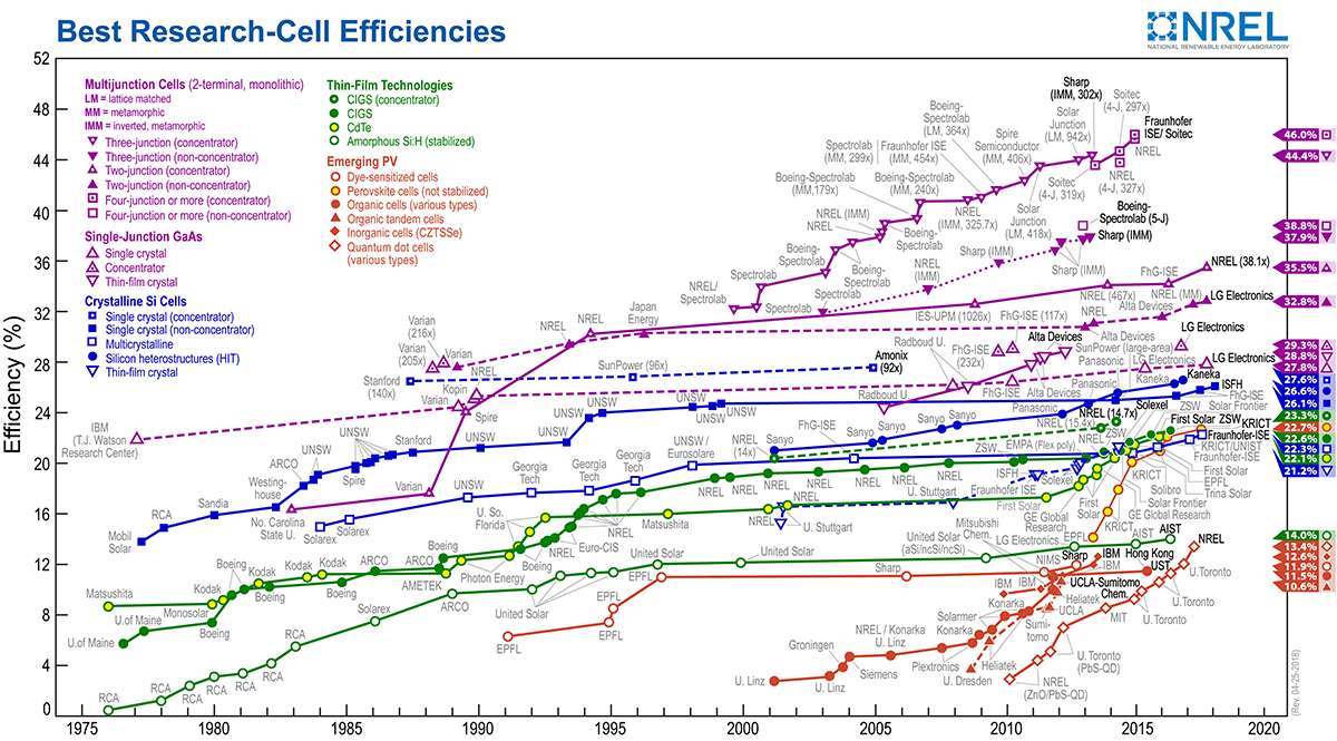
Hybrid organic–inorganic perovskites (HOIPs) are an exciting class of emergent materials that exhibit extremely promising photovoltaic (PV) properties.1 Among solution processable solar cell materials, HOIPs are—by far—the most efficient PV devices, with over 22% photovoltaic conversion efficiencies (PCEs).2 This combination of high efficiency and ease of fabrication promises a more readily scalable approach to solar cell manufacturing.3,4 HOIPs form a sub-set of a larger class of perovskite materials, all of which exhibit an ABX3 configuration. In HOIPs, the B-sites are occupied by metal cations (invariably, Pb, but sometimes Sn, or a mixture of both). A-site cations can be organic or inorganic in nature, and are typically methylammonium (MA), formamidinium (FA), or cesium (Cs). X denotes a choice of halide (Cl, Br, and/or I). These perovskites are usually processed in a solvent blend (S0:S1).1,4,5 In this paper, we will focus on the following commonly used HOIP solvents: Tetrahydrothiophene 1-oxide (THTO), dimethyl sulfoxide (DMSO), dimethylformamide (DMF), N-methyl-2-pyrrolidone (NMP), γ-butyrolactone (GBL), acetone, methacrolein, and nitromethane.
An exceedingly large combinatorial space thus exists from which HOIP salts can be fabricated. In principle, any combination of these species are possible, such as mixing 5% CsI with the binary HOIP blend of (FAPbI3)0.83 and (MAPbBr3)0.17.4,6,7,8 In addition, the choice of solvent is critical for producing high-quality films; hence, a wide variety of solvents, both pure and blended, have been studied (e.g., DMSO, DMF, GBL, NMP).9,10,11,12 Despite intense experimental scrutiny of many combinations of these species and different solvent processing protocols, there is no way to know whether a currently untested, but higher performing, material might exist, one comprised of an alternative combination of A-site cation, B-site cation, halide, and solvent blend.
We illustrate this combinatorial growth of the search space: Suppose we choose our HOIP candidate from among three A-site cations (MA, FA, Cs), one B-site cation (Pb), three X-site halides, all of which are constrained by 10% increments (e.g., MA0.9Cs0.1 is allowed, but not MA0.99Cs0.01), and allowing binary blends of solvents (from a reduced list of only eight solvent choices) of \({\textstyle{1 \over 3}}\) as the smallest ratio increments (allowing for 1:1:1 as the largest mixture). In that case, we would be faced with considering 522,720 possible combinations of species from which to form our ideal HOIP material.
We are interested in understanding molecular-scale interactions in solution. Unfortunately, no sufficiently accurate parameterized force field currently exists to model HOIP systems, essentially removing molecular dynamics (MD) as a viable information source for this high-fidelity investigation.13,14 As a result, we will restrict ourselves to using accurate ab initio density functional theory (DFT) to capture this information.15,16
To probe the solution processing of species that ultimately form thin films of perovskites, understanding the solubility of HOIP reagents in a so-called “bath” solvent is an important first step. Ideally, optimizing the enthalpy of solvation would be used as the metric by which to evaluate the ideal set of species that leads to the greatest solubility. However, an accurate estimate of the enthalpy of solvation requires the consideration of a full solvation shell around the lead salt, which can take weeks (or months) to compute using DFT. An appealing alternative is to use the Unsaturated Mayer bond order (UMBO), laid out by Stevenson et al.,17 as a measure of effective solubility. In contrast to enthalpy of solvation calculations, the UMBO typically takes only hours to compute, with the calculation time depending on the composition of the mixture and the level of theory used for the DFT. However, the UMBO is a descriptor that was solely designed for pure solvents, not solvent blends. As such, a good starting objective for validation purposes would be the limiting case of the enthalpy of solvation: the intermolecular binding energy between a perovskite salt (ABX3) and a pure solvent (S0).
Results
In the first test case, we searched the perovskite compositional space for an ABX3 combination with optimal intermolecular binding energy to a solvent molecule, S0. Note that only compositions with “pure” halides are considered, that is, all three halides are the same element. Each system contains a single halide, cation, central ion, and a pure solvent molecule. Hence, there exists a total number of 72 combinations. Using our approach, the Physical Analytics pipeLine (PAL), the intermolecular binding energy of a pure halide ABX3 − S0 was optimized, as shown in Fig. 1. The “optimal” mixture was found to be MAPbI3 in THTO.

Predictions of the binding energy between ABX3 and three solvent molecules during a single run of PAL to find the lowest energy for a given ABX3 composition (A ∈ {MA, FA, Cs} and X ∈ {Cl, Br, I}). The blue line depicts the binding energy of the composition recommended by PAL after iteration t = 1, …, 50 to the solvent. The red line gives the optimal binding energy of all 72 combinations, found by DFT calculations, thus identifying the optimal ABX3 − S0 mixture. PAL finds the optimal combination after about 12 iterations (16% of the 72 possible options). This particular demonstration was performed for five solvents. The molecule shown is an example of one such combination
In the second test case, a full-scale Bayesian optimization was run while also considering mixed halide systems (e.g., a Br/Cl/I mix). This involves a total of 240 possible combinations. An exhaustive search of all options was made using DFT calculations to provide a target (optimal) binding energy for validation purposes, as in test case 1. Starting with a randomly sampled combination, we iteratively update our hyperparameters until 10 total samples have been made. We then optimize hyperparameters every subsequent 10 iterations until we found the HOIP composition that minimized the ABX3 − S0 intermolecular binding energy (maximizing its magnitude). As seen in Figs. 2 and 3, the Bayesian optimization method identified a HOIP-solvent combination that produced a maximal target value within 50 iterations, with a mean of 31 and a standard deviation of 9 (averaged over 1000 replications). We also compare the results of our new method against a state-of-the-art optimization approach, pySMAC, as well as two Bayesian optimization methods that use Gaussian process (GP)-based models for the objective and differ in their handling of categorical variables (see below for details). Moreover, we compare to a random search:18
-
pySMAC19,20 is a highly optimized Bayesian optimization technique originally developed for the automated configuration of mathematical optimization algorithms. Its statistical model, based on random forests,21,22 is able to handle categorical variables, making it eligible to optimize over combinatorial spaces. pySMAC also employs the expected improvement acquisition criterion.
-
Simple BO follows a standard approach in Bayesian optimization and uses a standard GP model combined with the expected improvement acquisition function. Note that the latter is also employed by PAL. Simple BO incorporates categorical variables via “one-hot” encoding commonly used in Bayesian optimization, for example, in Google’s vizier.23
-
Hutter BO uses a tailored kernel for categorical variables that was proposed by Hutter in his Ph.D. thesis24 and follows Simple BO otherwise.
-
Random search18 picks an as-yet unevaluated combination uniformly at random in each iteration.

Test case 2: Bayesian optimization of the ABX3 HOIP-solvent intermolecular binding energy (A ∈ {MA, FA, Cs} and X ∈ {Cl, Br, I}). In this instance, we considered mixed halides. All 240 possible combinations of the binding energy were simulated using DFT calculations in order to find the most negative (and most favorable) binding energy, which is shown as a horizontal red line. Here, the optimal value for the binding energy was achieved in under 20 iterations (this may vary depending on initial sampled points)

Performance evaluation of PAL, Simple BO, Hutter BO, pySMAC, and random searches for the minimization of the intermolecular ABX3-solvent binding energy (maximizing its strength).44 PAL obtains a global optimum binding energy at considerably lower cost than the other methods. A shaded region of ±2 standard errors (SE) is shown for each method
The optimization process was replicated for multiple randomly chosen initial data sets. PAL, Simple BO, Hutter BO, and pySMAC were run for a thousand replications each, and Random for one million replications. The results of these evaluations are depicted in Fig. 3 and Table 1. The x-axis of Fig. 3 shows the number of observed points of each algorithm and the y-axis the binding energy of the best composition found after t iteration. We plot the highest found mean binding energy ±2 standard errors.
We observed that pySMAC initially obtains better combinations than any other method; however, PAL consistently obtains the global optimum first. That is, PAL involves the lowest number of DFT computations to find the best perovskite composition. Further, we can see the benefit of our statistical model when comparing PAL to Simple BO, in which PAL achieves global optimization in a under half the number of iterations than that of Simple BO (when comparing 99.9th percentile). Hutter BO performs worse than Simple BO. This is somewhat unexpected as Hutter BO uses a tailored covariance function designed for combinations of real-valued and categorical variables, whereas Simple BO uses an ad hoc encoding. Note that while both GP-based optimization methods perform worse than pySMAC initially, they require less steps to find an optimum on average (see Table 1 for details). All methods beat Random search eventually.
Discussion
We have proposed a new Bayesian optimization approach that overcomes challenges unique to materials discovery. While Bayesian optimization is commonly used for problems in machine learning and engineering with continuous rectangular search spaces, the specific perovskite design problem that we consider, in common with many chemical design problems, has search spaces with binary variables, indicating the presence or absence of a constituent species. Another critical challenge in this system is that the data are particularly scarce since the evaluation of a single design is often expensive, whether determined computationally or experimentally.
For challenging situations like these, we have demonstrated the promise of a Bayesian optimization approach that maximizes (or minimizes) an objective function, in this case, maximizing the intermolecular binding energy, to explore the combinatorial space of HOIP lead ion solvation. Our two test cases have demonstrated an improvement of close to 90% compared to that of an exhaustive search of 240 possible combinations of mixed-halide HOIP space. The same optimal compositions were found with both the Bayesian optimization prediction and the ab initio calculations. In addition, some of the top performers predicted by the Bayesian optimization approach have been found experimentally to be promising HOIP materials. Other, more unexpected, candidates promise potentially high-performing ABX3 − S0 mixtures that we suggest should be tested using experimental studies to validate these Bayesian optimization/DFT predictions. The improvement to Bayesian optimization using our Linear Belief model, laid out in the section “Linear Belief model”, suggests that atomic components contribute additively toward functions of cohesive energy. This can be seen by the considerable improvement of PAL over alternative benchmarked methods (pySMAC, Simple BO, Hutter BO, and Random). While we demonstrate our work in the context of HOIPs, the proposed methodology represents an advance that is broadly applicable for other materials design problems and constitutes a powerful new tool for the optimization of the design of chemical systems.
Applying Bayesian maximization of the intermolecular binding energy allowed us to predict the optimal HOIP–Solvent mixture (in a pure halide system), which was found to be MAPbI3 in THTO. This prediction corresponds well with the prevalence of experimental studies of MAPbI3 in the literature, in which it has been considered one of the best-performing compositions.3,25,26 In addition, experiments by Choi et al. have shown the particular efficacy of the THTO additive to dissolve Pb, corroborating these BO-guided/DFT-driven predictions.27
The caliber of the prediction for the mixed halides case is more difficult to evaluate since the experimental community has not yet decided on an optimal composition, probably because the number of options is overwhelming. Our Bayesian optimization studies predicted the maximized intermolecular binding energy to occur between FAPbI2Cl and THTO. This specific mixture of halides in conjunction with FA is unlike those normally studied experimentally. This, in itself, is an interesting result since the Bayesian optimization has clearly found a “disruptive” prediction. Once more, we find that THTO is a superior additive for dissolving ABX3.26,27
It is important to note that the Bayesian search produces a ranked list in which a number of candidates may produce close-to-optimal suggestions that meet the target value within the uncertainty of the methodology. That is true in this case, where four compositions are the highest performers with binding energies within 0.84 kJ/mol (0.2 kcal/mol) of each other, making them essentially inseparable. These candidates are FAPbI2Cl, MAPbI3 (an experimentally known high performer), and CsPbI3 in THTO, and finally CsPbICl2 in DMSO. All these candidates are predicted to be excellent choices, and notice that two of the four favor a single (rather than a mixed) halide. The ranked list serves a second, practical purpose, it predicts combinations not worth testing in the laboratory if complexation is the metric for success.
The choice of the objective function is crucial when employing Bayesian optimization and is a user-supplied aspect of our method. If, for example, we had chosen to optimize the photovoltaic conversion efficiencies (PCE), then the solvent would not be a factor, as the crystal exhibiting the PCE is solvent-free; this assumes that a single crystal is formed during the solution processing, in which the presence of solvent is important. If the objective were to find the most readily crystallized HOIP–Solvent combination, we would need to take more than the intermolecular binding energy into account.
Our model can readily be extended to take into account mixed ions and mixed halides/cations (e.g., 92% MA and 8% Cs) and beyond a 1:1:1 ratio of halide mixing. Our future work will investigate mixed solvents, for which mixing rules will need to be defined in order to provide appropriate solvent descriptors of density and permittivity, or an alternative descriptor.
Methods
In this section, we outline the design of PAL, which incorporates any test cases we may ultimately want to study, the Bayesian optimization approach, and finally the way that the PAL code implements this Bayesian approach.
Test cases
DFT calculations are sufficiently computationally intensive that an exhaustive computational search will generally be intractable, unless the compositional space is constrained sufficiently to make a validation study possible. We conducted two such tractably constrained, proof-of-concept studies that highlight the efficacy of using a Bayesian optimization approach to accelerate the search for an optimal HOIP composition.
Pure halides
Our first proof-of-concept was small enough in scope to allow us to validate the Bayesian optimization prediction of the optimal HOIP composition by comparison to an exhaustive search using DFT. This test case sought the optimal pure halide perovskite that maximizes the lead ion's solubility. In our model, a perovskite “composition” consists of four major components: a halide anion, an A-site cation, one pure solvent, and a lead cation (B-site) that serves as the central ion of the cluster. The halide anions are selected among I, Br, or Cl. The A-site cation can be MA, FA, or Cs. For the solvent, we considered only one of eight common pure solvent choices: THTO, DMSO, DMF, NMP, GBL, acetone, methacrolein, and nitromethane. The solubility was approximated as the intermolecular binding energy between ABX3 and N solvent molecules (for benchmarking purposes, 3 was chosen), which we can reasonably assume to be positively correlated with the enthalpy of solvation (Hsolv).
A given perovskite composition can be described by an eight-dimensional vector \(x \in {\Bbb X}\), where \({\Bbb X} = \{ 0,1\} ^6 \times {\Bbb R} \times {\Bbb R}\). x1:6 are binary values that together indicate the presence of a particular halide in the solution. We require that \(\mathop {\sum}\nolimits_{i = 1}^3 {\kern 1pt} x_i = 1\), and the non-zero xi indicates that the corresponding halide is present. For example, (0, 1, 0) indicates a perovskite salt of ABBr3. x4:6 are also binary values that together indicate the presence of a particular cation. Similarly, we require \(\mathop {\sum}\nolimits_{i = 4}^6 {\kern 1pt} x_i = 1\), in which the non-zero xi indicates that the corresponding cation is present. x7 and x8 are real-valued solvent descriptors with x7 being the relative dielectric (εr) and x8 the density (ρ). Since the lead ion is present in every composition, it is omitted here in the description of x. Note that different central ions (e.g., Sn instead of Pb) could be added to the description in a similar fashion. We remark that we neglect x8 when we compare PAL to the other baseline methods, which results in a slightly worse performance of PAL. That is, the PAL described in this section performs even somewhat better than in the performance plot. This is done to allow for a fair comparison between PAL and pySMAC, as pySMAC does not support discrete variable that take value in a finite set of pairs of reals.
Mixed halides
For the more challenging mixed halide case study, we extended the perovskite composition vector x to be \(x \in {\Bbb Y}\), where \({\Bbb Y} = \{ 0,1\} ^{12} \times {\Bbb R} \times {\Bbb R}\). x1:9 are binary values that together indicate the presence of a particular halide in the solution. We require that \(\mathop {\sum}\nolimits_{i = 1}^3 {\kern 1pt} x_i\) = \(\mathop {\sum}\nolimits_{i = 4}^6 {\kern 1pt} x_i\) = \(\mathop {\sum}\nolimits_{i = 7}^9 {\kern 1pt} x_i\) = 1, and the non-zero xi indicates that the corresponding halide is present in the solution. For example, (0, 1, 0, 0, 1, 0, 1, 0, 0) indicates a perovskite salt of ABBr2I. x10:12 are also binary values that together indicate the presence of a particular cation. Similarly, we require \(\mathop {\sum}\nolimits_{i = 10}^{12} {\kern 1pt} x_i = 1\) and the non-zero xi indicates that the corresponding cation is present in the solution. x13 and x14 are real-valued solvent descriptors with x13 being the relative dielectric (εr) and x14 the density (ρ). Since the lead ion is present in every composition, it is again omitted from x. Once again, we neglect x14 when benchmarking PAL with the state-of-the-art methods .
Bayesian optimization
Bayesian optimization has emerged as a powerful technique to find an optimizer of expensive-to-evaluate functions.28,29 It consists of two components: a surrogate model for the objective function and an acquisition function for selecting the next sample point. The Bayesian optimization algorithm proceeds as follows:
-
1.
Using an inital data set, estimate the hyperparameters of the prior for the components of the Linear Belief model. When benchmarking, start with only a single point.
-
2.
Compute the posterior probability distribution, given the prior and the initial data.
-
3.
Until the budget for samples is exhausted, do in iteration t:
-
(a)
Select the next combination x(t) to sample via the acquisition function.
-
(b)
Evaluate the objective value of x(t).
-
(c)
Update the posterior with the new observation.
-
(d)
On a regular schedule, estimate the hyperparameters again, using all gathered observations.
-
(a)
-
4.
Return the best found combination.
The decision to recommend the combination with the best objective value among the sampled candidates is conservative from a decision-theoretic perspective and natural for noise-free observations.
In what follows, we propose a statistical model tailored for perovskite compositions. For the acquisition function, we selected the expected improvement approach that is known to perform well when objective values can be observed without noise, as here.30,31
Linear Belief model
We assume that the four components (Pb, A-site cation, halide, and solvent) contribute to the binding energy of a perovskite-solvent mixture in an additive manner. The actual effect of each component is unknown and will be inferred from observations (i.e., from DFT calculations of the binding energy). This is akin to the generalized Free-Wilson approach that was successfully used to predict biological activity; however, we further expand on this approach by also drawing from a Gaussian Process (GP).32
We apply Bayesian linear regression and suppose that the binding energy of the composition corresponding to x is given by V(x), as outlined in Eq. (1):
Here n indicates the number of binary descriptors for the ABX3 salt: 6 in pure halides and 12 in mixed halides. αi is the contribution to the binding energy of xi made by the presence of halides and cations, and is assumed to be the same for all halides and cations. β(x) captures the deviation of V(x) from the linear model. ζ represents the contribution of the common lead cluster. f(xε, xρ) captures the contribution of the solvent S0 to the binding energy (in pure halides xε = x7 and xρ = x8, in mixed halides xε = x13 and xρ = x14). The contribution of the solvent as a function of the dielectric and the density is represented by xε and xρ, respectively.
Prior distribution
In accordance with the Bayesian paradigm, we place a prior distribution on the components of the regression model. We suppose that each \(\alpha _i\sim N\left( {\mu _\alpha ,\sigma _\alpha ^2} \right)\), i.e., the coefficients are independent and identically distributed, conditioned on μα and \(\sigma _\alpha ^2\). Moreover, we suppose that the non-linear correction for every x has prior \(\beta (x)\sim N\left( {0,\sigma _\beta ^2} \right)\) and that \(\zeta \sim N\left( {\mu _\zeta ,\sigma _\zeta ^2} \right)\).
We employ GP regression to capture the contribution of the solvent blend. We suppose that f(·) is drawn from a GP with prior mean function μ0(·) and covariance Σ0(·, ·). Since ζ captures the invariant contribution from the central ion, it is reasonable for us to assume μ0(·) = 0. Finally, we assume different solvents will behave similarly if their descriptors are similar. This is formalized in the use of the 5/2 Matérn Kernel. Let Si = (xε,i, xρ,i) and \(r = \sqrt {\mathop {\sum}\nolimits_{i = 1}^d {\kern 1pt} l_i\left( {S_{1,i} - S_{2,i}} \right)^2}\) denote the “similarity” between solvents S1 and S2, with dimensions weighted by li. Note that in our model d = 2.
The covariance of two solvent blends S1 and S2 is then given as:
Thus, the proposed generative model has the hyperparameters:
Our prior distribution on V1, V2, …, Vn is multivariate normal with mean μ0 and covariance function Σ0:
Note that μ0 at x equals:
and the covariance \({\mathrm{\Sigma }}_{x,x\prime }^0\) of x and x′ under the prior is given by:
where Im is the m × m identity matrix, and Jm is the m × m matrix of ones. Here we introduce the bra-ket notation for a column vector, |x〉, or a row vector, 〈x|. As such, 〈x|x〉 would be a scalar, and |x〉 〈x| an m × m matrix, where m is the length of the |x〉 vector. Finally, subscripts are inclusive; that is, 〈x1:3| = (x1, x2, x3).
Hyperparameter fitting and posterior
The hyperparameters of our model, as summarized in Eq. (3), are estimated from data. For the experimental evaluation, we used a maximum likelihood estimate, using an initial dataset sampled according to a Latin Hypercube design and subsequently optimized via an L-BFGS-B approach. The optimized sampled hyperparameters that behave the best are then chosen. We suppose that the objective value of any x can be observed without noise. Then the posterior distribution of f(·), the contribution of the solvent blend, is multivariate normal and so is the posterior distribution of the coefficients of the regression model.33
Validation of the model
We validate the Linear Belief model described above by the leave-one-out cross-validation (LOO-CV) method (see Fig. 4). Moreover, leave-p-out cross-validation (LpO-CV) was also performed in which p = 100 data points are removed from the training set for validation purposes (see Fig. 4). These validations demonstrate that the proposed regression model well represents the intermolecular binding energies from DFT.

Cross-validation using a LOO-CV method (left) and a LpO-CV method (right). The black line shows the values obtained from DFT calculations. The blue line shows the predictive mean of the proposed regression model, whose hyperparameters were trained on either (1) all data points excluding the one being predicted (LOO-CV) or (2) 140 data points, and then tested against the 100 remaining. The y-axis shows the intermolecular binding energy
The PAL
The PAL, illustrated in Fig. 5, is a Python-based framework that we have designed for the task of maximizing a chosen computational objective as a function of a material’s composition. Bayesian optimization lends itself to consideration of expensive objective functions and, as such, provides several possibilities for DFT calculations.28,29

The Physical Analytics pipeLine. On the left, objective functions from simulations are fed into the Bayesian optimization code (middle of the schematic) to produce ranked predictions of ABX3–Solvent mixtures of interest (rightmost cartoon). Experimental sources of information (top schematic) can ultimately be used for further validation, as well as further fine-tuning of the statistical model
Thus, PAL combines the functionality of Bayesian optimization, using the generative model proposed in the section “Bayesian optimization”, with a refined method to calculate the enthalpy of solvation or other metric of success. In order to ensure the robustness of PAL, the code was written to accommodate calculations of other options, including (1) solvation, (2) intermolecular attractions, (3) steric hinderance, and (4) molecular properties. As such, the following choices are considered for the objective function:
-
1.
The Unsaturated Mayer Bond Order (UMBO) within a solvent molecule (from the most polar atom to its nearest intra-molecular neighboring atom).
-
2.
The intermolecular binding energies.
-
3.
The volume and eccentricity of a solvent or solute, defined by a Minimum Volume-Enclosing Ellipse (MVEE).34
-
4.
The dipole moment of a solvent.
Unsaturated Mayer bond order
In order to capture the UMBO between solvent and solute, where the solute is some HOIP species ABX3 (with A being a cation, B being either Pb or Sn, and X a halide), we must first isolate a stable geometric configuration of these molecules. This is accomplished by equilibrating a large box of solvents using MD, of which a smaller sub-system is further equilibrated (within MD), and finally the specific motif (within the sub-system) is geometry-optimized in DFT. The initial two MD steps are performed in order to automate the generation of an adequate starting configuration for the subsequent DFT optimization. To make the large solvent box, we used the packmol software to pack together a single lead salt solute in a 25 × 25 × 25 Å3 box of solvent.35 From this starting point, the MD calculations were done in LAMMPS, a popular MD software, with the OPLS-AA Force Field.36,37 Since we plan to perform an accurate DFT geometry optimization of a proposed configuration, we allow for the following assumptions within our MD simulations:
-
1.
We can run an equilibration using the microcanonical, NVE, ensemble with a limited step size as a way to circumvent the risk of an unexpectedly poor starting state.
-
2.
We need only run the NVE and isobaric-isothermal, NPT, equilibrations for 10,000 iterations (10 ps).
-
3.
The large box (in MD) is equilibrated using the NVE ensemble with a 0.1 Å limited step size, and is followed up by equilibration using the NPT ensemble at 300 K and 1 atm.
-
4.
The smaller box (in MD) is equilibrated using the NVE ensemble with a 0.001 Å limited step size, and is followed up by another NVE ensemble equilibration with a 0.01 Å limited step size.
-
5.
We approximate Pb as Ba in OPLS-AA, as they have the same oxidation state (+2). This is because Pb is not parameterized in this force field.
-
6.
We hold ABX3 constant by removing forces throughout the MD simulations.
-
7.
A time step of 1.0 fs is reasonable, especially with the limited step sizes of the NVE calculations.
The smaller MD simulation box is derived from the larger simulation box (post-equilibration) by first determining the intermolecular distances from the solute ion (in our case, Pb) to the most polar atom within the solvents (typically oxygen). From this, either the closest N solvents can be chosen, or all solvents within a given radius. In the case where we use the UMBO as the basis for our objective function, we consider the closest solvent molecule.
The final geometry is then optimized using the B97-D3 GGA basis set with Grimme’s dispersion correction.38,39 The def2-TZVP basis set is used, with an effective core potential for the Pb ion.40 Whenever a solvent is simulated, both an explicit solvent and implicit solvent model (using the COSMO package) are used.41 This is done because the implicit model is a low-cost method to improve/incorporate the electronic polarization of the solute.42 The system, as well as individual components (solute and solvent), are optimized in the Orca DFT package, with the final UMBO being returned as an output.43
Binding energy
In a similar fashion to the UMBO calculation, we begin with an equilibration of a large solvent box. Here, however, instead of considering only one solvent, we isolate the N nearest neighbor solvent molecules to a given ABX3 solute. Finally, in order to accomplish a binding energy calculation, we also need the energy of the individual systems of interest. In the case of ABX3 or a single solvent, we simply optimize the molecule independently in DFT. However, in the case of N mixed solvents, we must use the same procedure as that used when isolating a stable geometric configuration for the solvent-solute system: a large MD equilibration of a solvent box, followed by a smaller MD equilibration of N solvents, followed by a DFT geometry optimization of the final system.
As such, PAL is capable of calculating the following intermolecular binding energies:
-
1.
S0 vs. S0,
-
2.
S0 vs. S1,
-
3.
S0 vs. ABX3, and
-
4.
S0,S1, …, Sn vs. ABX3.
Steric hinderance
Steric hinderance, shortened hereafter as “sterics”, captures the effect of volume exclusion effects due to the presence of the molecules. This can cause issues with molecular packing and induce strain within large molecular systems. In the case of nucleation, sterics comes into play as the physical restrictions involved when reactive species approach one another. As such, defining order parameters to capture the effects of sterics in relation to (a) solvation or (b) reactivity is relevant. One such approach is to define a MVEE around molecules to abstract the globularity of the molecule and ultimately simplify the problem.34 With an ellipse describing the molecule, a variety of mathematical representations are now available, including volume, eccentricity, and surface area. Alone, these values may be of use, but it is likely that a combination with other molecular properties would prove even more useful.
Molecular properties
Beyond calculations of molecular interactions (e.g., the UMBO, binding energy, or steric hinderance), molecules themselves possess characteristic properties (such as polarization and density) that contribute to their bulk behavior. Some of these properties remain accessible at the DFT level, allowing us to use them within suitably constructed objective functions (such as the Gutmann donor number, which was recently shown to be a potential indicator of Pb solubility).9 Although it has been shown that not all commonly used molecular properties directly correlate with bulk properties of interest, an objective function coupling them to molecular interactions may prove useful.17
Data availability
The code for this article and the results of the DFT calculations are publicly available at https://github.com/clancyLab/NCM2018.
References
Brenner, T. M., Egger, D. A., Kronik, L., Hodes, G. & Cahen, D. Hybrid organic-inorganic perovskites: low-cost semiconductors with intriguing charge-transport properties. Nat. Rev. Mater. 1, 1–16 (2016).
National Renewable Energy Laboratory. Best research-cell efficiencies. https://www.nrel.gov/pv/assets/images/efficiency-chart.png (2018).
Yang, S., Fu, W., Zhang, Z., Chen, H. & Li, C.-Z. Recent advances in perovskite solar cells: efficiency, stability and lead-free perovskite. J. Mater. Chem. A 5, 11462–11482 (2017).
Yang, W. S. et al. Iodide management in formamidinium-lead-halide-based perovskite layers for efficient solar cells. Science 356, 1376–1379 (2017).
Eames, C. et al. Ionic transport in hybrid lead iodide perovskite solar cells. Nat. Commun. 6, 1–8 (2015).
Kim, C., Huan, T. D., Krishnan, S. & Ramprasad, R. A hybrid organic-inorganic perovskite dataset. Sci. Data 4, 1–11 (2017).
Rolston, N. et al. Effect of cation composition on the mechanical stability of perovskite solar cells. Adv. Energy Mater. 8, 1–7 (2017).
Xu, F., Zhang, T., Lia, G. & Zhao, Y. Mixed cation hybrid lead halide perovskites with enhanced performance and stability. J. Mater. Chem. A 5, 11450–11461 (2017).
Hamill, J. C. Jr., Schwartz, J. & Loo, Y. L. Influence of solvent coordination on hybrid organic-inorganic perovskite formation. ACS Energy Lett. 3, 92–97 (2018).
Zhou, Y. et al. Manipulating crystallization of organolead mixed-halide thin films in antisolvent baths for wide-bandgap perovskite solar cells. ACS Appl. Mater. Interfaces 8, 2232–2237 (2016).
Yoon, S., Ha, M.-W. & Kang, D.-W. PCBM-blended chlorobenzene hybrid anti-solvent engineering for efficient planar perovskite solar cells. J. Mater. Chem. C 5, 10143–10151 (2017).
Gardner, K. L. et al. Nonhazardous solvent systems for processing perovskite photovoltaics. Adv. Energy Mater. 6, 1–8 (2016).
Mattoni, A., Filippetti, A., Saba, M. I. & Delugas, P. Methylammonium rotational dynamics in lead halide perovskite by classical molecular dynamics: The role of temperature. J. Phys. Chem. C 119, 17421–17428 (2015).
Gutierrez-Sevillano, J. J., Ahmad, S., Caleroa, S. & Anta, J. A. Molecular dynamics simulations of organohalide perovskite precursors: solvent effects in the formation of perovskite solar cells. Phys. Chem. Chem. Phys. 17, 22770–22777 (2015).
Tsipis, A. C. DFT flavor of coordination chemistry. Coord. Chem. Rev. 272, 1–29 (2014).
Burns, L. A., Vázquez-Mayagoitia, A., Sumpter, B. G. & Sherrill, C. D. Density-functional approaches to noncovalent interactions: a comparison of dispersion corrections (DFT-D), exchange-hole dipole moment (XDM) theory, and specialized functionals. J. Chem. Phys. 134, 084107 (2011).
Stevenson, J. et al. Mayer bond order as a metric of complexation effectiveness in lead halide perovskite solutions. Chem. Mater. 29, 2435–2444 (2017).
Bergstra, J. & Bengio, Y. Random search for hyper-parameter optimization. J. Mach. Learn. Res. 13, 281–305 (2012).
Hutter, F., Hoos, H. H., & Leyton-Brown, K . in Learning and Intelligent Optimization (ed Coello, C.A.C.) 507–523 (Springer, Berlin, Heidelberg, 2011).
Falkner, S. pySMAC. https://github.com/sfalkner/pySMAC (2016).
Ho, T. K. Random decision forests. In: (ed Kavanaugh, M. & Storms, P.) Proceedings of the Third International Conference on Document Analysis and Recognition, 278–282, IEEE: Montreal, Canada (1995).
Ho, T. K. The random subspace method for constructing decision forests. IEEE Trans. Pattern Anal. Mach. Intell. 20, 832–844 (1998).
Golovin, D. et al. (eds.) Google vizier: a service for black-box optimization. http://www.kdd.org/kdd2017/papers/view/google-vizier-a-service-for-black-box-optimization (2017).
Hutter, F. Automated Configuration of Algorithms for Solving Hard Computational Problems. Ph.D. thesis, University of British Columbia (2009).
Grancini, G. et al. One-year stable perovskite solar cells by 2D/3D interface engineering. Nat. Commun. 8, 1–8 (2017).
Giesbrecht, N. et al. Single-crystal-like optoelectronic-properties of MAPbI3 perovskite polycrystalline thin films. J. Mater. Chem. A 6, 4822–4828 (2018).
Foley, B. J. et al. Controlling nucleation, growth, and orientation of metal halide perovskite thin films with rationally selected additives. J. Mater. Chem. A 5, 113–123 (2016).
Brochu, E., Cora, V. M. & de Freitas, N. A tutorial on Bayesian optimization of expensive cost functions, with application to active user modeling and hierarchical reinforcement learning. arXiv:1012.2599 (2010).
Shahriari, B., Swersky, K., Wang, Z., Adams, R. P. & de Freitas, N. Taking the human out of the loop: a review of Bayesian optimization. Proc. IEEE 104, 148–175 (2016).
Jones, D. R., Schonlau, M. & Welch, W. J. Efficient global optimization of expensive black-box functions. J. Glob. Optim. 13, 455–492 (1998).
Snoek, J., Larochelle, H. & Adams, R. P. Practical Bayesian optimization of machine learning algorithms. Adv. Neural Inf. Process. Syst. 2951–2959 (2012).
Negoescu, D. M., Frazier, P. I. & Powell, W. B. The knowledge-gradient algorithm for sequencing experiments in drug discovery. INFORMS J. Comput. 23, 346–363 (2011).
Gelman, A. et al. Bayesian Data Analysis, Third Edition (Chapman & Hall/CRC Texts in Statistical Science) (Chapman and Hall/CRC, London, 2013).
Todd, M. J. & Yldrm, E. A. On Khachiyan's algorithm for the computation of minimum-volume enclosing ellipsoids. Discret. Appl. Math. 155, 1731–1744 (2007).
Martínez, L., Andrade, R., Birgin, E. G. & Martínez, J. M. Packmol: a package for building initial configurations for molecular dynamics simulations. J. Comput. Chem. 30, 2157–2164 (2009).
Plimpton, S. Fast parallel algorithms for short-range molecular dynamics. J. Comp. Phys. 117, 1–19 (1995).
Jorgensen, W. L., Maxwell, D. S. & Tirado-Rives, J. Development and testing of the OPLS all-atom force field on conformational energetics and properties of organic liquids. J. Am. Chem. Soc. 118, 11225–11236 (1996).
Grimme, S. Semiempirical GGA-type density functional constructed with a long-range dispersion correction. J. Comp. Chem. 27, 1787–1799 (2006).
Grimme, S., Ehrlich, S. & Goerigk, L. Effect of the damping function in dispersion corrected density functional theory. J. Comput. Chem. 32, 1456–1465 (2011).
Weigend, F. & Ahlrichs, R. Balanced basis sets of split valence, triple zeta valence and quadruple zeta valence quality for H to Rn: design and assessment of accuracy. Phys. Chem. Chem. Phys. 7, 3297–3305 (2005).
Marenich, A. V., Cramer, C. J. & Truhlar, D. G. Universal solvation model based on solute electron density and on a continuum model of the solvent defined by the bulk dielectric constant and atomic surface tensions. J. Phys. Chem. B 113, 6378–6396 (2009).
Cramer, C. J. & Truhlar, D. G. Implicit solvation models: equilibria, structure, spectra, and dynamics. Chem. Rev. 99, 2161–2200 (1999).
Neese, F. The ORCA program system. WIREs Comput. Mol. Sci. 2, 73–78 (2012).
Neumann, M., Huang, S., Marthaler, D. E. & Kersting, K. pyGPs—a python library for Gaussian process regression and classification. J. Mach. Learn. Res. 16, 2611–2616 (2015).
Acknowledgements
This work was partially supported by the Cornell Center for Materials Research with funding from the NSF MRSEC program (DMR-1719875) through a seed funding award. H.H. and M.P. were partially supported by this award. P.C., P.F., W.H., and M.P. were partially supported by NSF (CMMI-1536895, DMR-1719875, DMR-1120296, CMMI-1254298) and by AFOSR (FA9550-15-1-0038). The Cornell Institute for Computational Science and Engineering is thanked for access to their computing resources.
Author information
Authors and Affiliations
Contributions
H.C.H. implemented PAL in its entirety (automated MD-DFT objective function), and incorporated the Bayesian optimization code into the package. W.H. implemented the initial proof-of-concept pure halide Bayesian optimization code, and H.C.H. further extended it to incorporate mixed halides. P.F. helped correct inaccuracies during the implementation of the Bayesian optimization. M.P. and P.C. were responsible for the overall design of the study and preparation of the manuscript. M.P. was also responsible for suggesting the tests of the statistical significance of the results. H.C.H., M.P., and P.C. wrote the manuscript. M.P. is the guarantor for this manuscript.
Corresponding author
Ethics declarations
Competing interests
The authors declare no competing interests.
Additional information
Publisher's note: Springer Nature remains neutral with regard to jurisdictional claims in published maps and institutional affiliations.
Electronic supplementary material
Rights and permissions
Open Access This article is licensed under a Creative Commons Attribution 4.0 International License, which permits use, sharing, adaptation, distribution and reproduction in any medium or format, as long as you give appropriate credit to the original author(s) and the source, provide a link to the Creative Commons license, and indicate if changes were made. The images or other third party material in this article are included in the article’s Creative Commons license, unless indicated otherwise in a credit line to the material. If material is not included in the article’s Creative Commons license and your intended use is not permitted by statutory regulation or exceeds the permitted use, you will need to obtain permission directly from the copyright holder. To view a copy of this license, visit http://creativecommons.org/licenses/by/4.0/.
About this article

Cite this article
Herbol, H.C., Hu, W., Frazier, P. et al. Efficient search of compositional space for hybrid organic–inorganic perovskites via Bayesian optimization. npj Comput Mater 4, 51 (2018). https://doi.org/10.1038/s41524-018-0106-7
Received:
Revised:
Accepted:
Published:
DOI: https://doi.org/10.1038/s41524-018-0106-7
- Springer Nature Limited
This article is cited by
-
High-throughput screening of catalytically active inclusion bodies using laboratory automation and Bayesian optimization
Microbial Cell Factories (2024)
-
Targeted materials discovery using Bayesian algorithm execution
npj Computational Materials (2024)
-
A multi-objective optimization based on machine learning for dimension precision of wax pattern in turbine blade manufacturing
Advances in Manufacturing (2024)
-
Discovery of Pb-free hybrid organic–inorganic 2D perovskites using a stepwise optimization strategy
npj Computational Materials (2022)
-
Benchmarking the performance of Bayesian optimization across multiple experimental materials science domains
npj Computational Materials (2021)