
Abstract
The extraction of objects from large-scale historical maps has been examined in several studies. With the aim to research urban changes over time, semi-automated and transferable holistic approaches remain to be investigated. We apply a combination of object-based image analysis and vectorization methods on three different historical maps. By further matching and georeferencing an appropriate current geodataset, we provide a concept for analyzing and comparing those valuable sources from the past. With minor adjustments, our end-to-end workflow was transferable to other large-scale maps. The findings revealed that the extraction and spatial assignment of objects, such as buildings or roads, enable the comparison of maps from different times and form a basis for further historical analysis. Performing an affine transformation between the datasets, an absolute offset of no more than 72 m was achieved. The outcomes of this paper, therefore, facilitate the daily work of urban researchers or historians. However, it should be emphasized that specific knowledge is required for the presented subjective methodology.
Zusammenfassung
Die Extraktion von Objekten aus großmaßstäbigen historischen Karten ist Gegenstand zahlreicher Forschungsprojekte. Um den urbanen Wandel im Laufe der Zeit zu untersuchen, bedürfen semi-automatisierte und holistische Ansätze jedoch weiteren Untersuchungen. In dieser Arbeit werden Methoden zur objektbasierten Bildanalyse und Vektorisierung auf drei verschiedene historische Karten angewendet. Mithilfe eines anschließenden Abgleichs sowie der Georeferenzierung eines entsprechenden aktuellen Geodatensatzes stellen wir ein Konzept vor, das sowohl die Analyse als auch den Vergleich der wertvollen Informationsquellen aus der Vergangenheit erlaubt. Nur geringfügige Änderungen waren notwendig, um den ganzheitlichen Arbeitsablauf auf andere großmaßstäbige Karten zu übertragen. Unsere Ergebnisse zeigten, dass die Extraktion und räumliche Zuordnung von Objekten wie Gebäude oder Straßen einen Vergleich zwischen Karten verschiedener Zeitalter ermöglichen und somit eine Grundlage für weitere historische Analysen schaffen. Im Zuge einer affinen Transformation ergab sich eine maximale Abweichung von 72 m zwischen beiden Datensätzen. Die Ergebnisse dieser Studie erleichtern damit die tägliche Arbeit von z. B. Stadtforschern oder Historikern. Dennoch sollte berücksichtigt werden, dass die vorgestellte subjektive Methodik spezifisches Fachwissen erfordert.
1 Introduction
Historical maps are valuable sources when investigating spatial changes over time (Herold 2018). As an essential tool for communicating geographic objects and their locations, they are often the only source of information for the understanding of spatio-temporal change (Sun et al. 2021; Kim et al. 2014). With large-scale maps (approx. > 1:20,000)—especially “city maps”—we are able to study urban morphology (Meinel et al. (2009), as cited in Muhs et al. 2016). Frequently, geographical, political, environmental, and other urbanization processes can be backtraced solely by means of historical maps.
For the analysis of the urban landscape of the past, it is inevitable to make the information from large-scale historical maps accessible. Single map objects may provide insights into former names of roads and buildings or their evolution over time. But generally, physical scans (bitmaps) of historical maps are not machine-readable. Manual attempts to acquire information from historical maps are not uncommon but error-prone, time-intensive, and non-transferable (Xydas et al. 2022; Chiang et al. 2020; Gobbi et al. 2019). There is a need for (semi-)automated approaches to solve these problems.
In this study, we provide a holistic workflow to not only extract objects from large-scale historical maps, but also to derive benefits from the entirety of geometric, relational, and semantic information. Moreover, our semi-automated approach demonstrates how a spatial assignment between historical and current maps may be enabled and therefore provides a basis for further comparison processes between these.
An established strategy used to semi-automatically extract objects from historical maps while minimizing the reader’s subjective influence starts with image segmentation, which follows the principles of human perception: objects within an image are differentiated due to graphical variations (e.g., in light intensity, texture, or spatial context), artifacts, and deviations. Visually homogeneous image areas form so-called segments. By combining object segmentation and classification, the concept of geographic object-based image analysis (GEOBIA) is able to reproduce physically existing objects, like buildings or roads, from raster maps (Herold 2018; Hussain et al. 2013; Hay and Castilla 2008; Neubert 2005). However, authors agree that “there is no single extraction method that can be effectively applied to all different historical maps” (Sun et al. 2021). This is a complex task and only few studies have shown suggestions for further processing and the applicability of their results.
Most research in this field aims at extracting and vectorizing geometries from historical maps to make them analyzable, but frequently comes with several limitations and preconditions. Many studies focus on the extraction of a single feature type such as streets (Chiang and Knoblock 2013; Chiang and Knoblock 2012), river bodies (Gede et al. 2020), or different land use classes (Gobbi et al. 2019; Zatelli et al. 2019) like forest areas (Ostafin et al. 2017; Herrault et al. 2013; Leyk et al. 2006) or wetlands (Jiao et al. 2020). Others assume homogeneously colored map regions (Chiang et al. 2011; Leyk and Boesch 2010; Ablameyko et al. 2002), which is rarely true for historical maps. Less complex (“binary”) maps containing homogeneously black objects or contours on white backgrounds were investigated by Xydas et al. (2022), Heitzler and Hurni (2020), Le Riche (2020), Iosifescu et al. (2016), Muhs et al. (2016), and Kim et al. (2014). But differentiating objects solely based on color differences is insufficient especially for widespread monochrome historical maps or due to ancient paper texture, noise, or dirt on the hand-drawn maps (Jiao et al. 2020; Peller 2018; Muhs et al. 2016; Arteaga 2013; Leyk and Boesch 2010). Labels often remain unconsidered in the context of object recognition from historical maps as they commonly suffer from overlaps or gray-scale values similar to textures or contours of other map elements (Heitzler and Hurni 2020; Peller 2018). Other authors presume an existing coordinate system (Le Riche 2020; Gobbi et al. 2019; Iosifescu et al. 2016) or a huge stock of training data, which is needed for machine learning approaches (Xydas et al. 2022; Heitzler and Hurni 2020; Jiao et al. 2020; Gobbi et al. 2019; Zatelli et al. 2019; Uhl et al. 2017). Moreover, few studies have focused on large-scale but rather small-scale maps (Gede et al. 2020; Heitzler and Hurni 2020; Gobbi et al. 2019; Zatelli et al. 2019; Loran et al. 2018; Uhl et al. 2017; Muhs et al. 2016; Herrault et al. 2013).
As existing research generally focuses on separate processes involved in object extraction from historical maps, our study suggests a holistic approach composed of extracting, vectorizing, and linking objects. We demonstrate the benefits of eliminating and assigning labels for this whole process and present applicabilities of the resulting geometries. Because only by considering these techniques as a whole, we are able to answer location-related questions on the evolution of geographic features and make historical maps “accessible to geospatial tools and, thus, for spatio-temporal analysis of landscape patterns and their changes” (Uhl et al. 2017). New qualitative and quantitative analyses as well as comparisons to other historical or current geodata become possible by searching through and processing information derived from historical maps (Gobbi et al. 2019; Chiang 2017; Iosifescu et al. 2016). For long-term backtracing of individual buildings, for instance, shape-based comparisons across different maps are useful (Le Riche 2020; Laycock et al. 2011).
In this work, we present a semi-automatic solution to make large-scale historical maps usable for spatial analysis while minimizing time-intensive and laborious manual user intervention. Based on our previous findings on the needs of users of historical maps (Schlegel 2019) as well as on the identification and extraction of map labels (Schlegel 2021), we demonstrate the general feasibility of a comprehensive workflow composed of (1) eliminating labels, (2) extracting geometries, (3) vectorizing and refining those, and (4) matching and spatially assigning the extracted map objects with current ones. Potential future applications, which are shown in the further course, may be involving semantic information from labels to annotate corresponding map features or an adjustment of a map’s visual appearance. Prospectively, new databases can be set up and comparative studies between different datasets become possible.
2 Literature Review
2.1 Elimination of Labels
Labels are valuable components in historical maps holding important metadata. However, text within a map is typically seen as a disturbing factor when extracting geometries. Misinterpretations in the context of segmentation may easily arise due to overlaps, direct adjacencies, or similar color values to map elements and structures such as lines or textures (Heitzler and Hurni 2020; Bhowmik et al. 2018; Chiang 2017). Monochrome maps, in particular, have a reduced number of parameters to differentiate between text and other elements. However, an initial elimination of text or labels from historical maps can be seen as a major advantage for further object extraction processes (Gede et al. 2020). Previous attempts identified labels with the help of text recognition—subsequent to object recognition and vectorization—or by shape recognition algorithms (Iosifescu et al. 2016). Chrysovalantis and Nikolaos (2020) used binarized maps to separate text from other objects (see also Bhowmik et al. (2018)). By eliminating small pixel groups, they were able to remove letters. A GRASS GIS add-on developed by Gobbi et al. (2019) and Zatelli et al. (2019) replaces relevant pixel values by means of low-pass filters within old cadaster maps. However, pixels must already be defined as “text” in advance. Telea (2004) and Bertalmío et al. (2001) suggest different image inpainting techniques, which are often applied for image restoration. Missing or damaged image regions are filled to create an image without giving the viewer a hint of changes. In our testing, these approaches caused an unsatisfactory blurring of the input image.
2.2 Object-Based Image Analysis
Many methodologies for (semi-)automated object extraction from historical maps were demonstrated in recent years but proven insufficient for various reasons. For instance, a common histogram thresholding or color space clustering (Herrault et al. 2013) ignores any spatial context, whereas artificial neural networks require an inadequate amount of training data (Gobbi et al. 2019).
Chrysovalantis and Nikolaos (2020) used GIS functionalities to convert a historical multicolor map into a binary image and then to extract and vectorize geometries of buildings. However, textured or corrupt polygons could not be handled and labels were eliminated only partially. A similar approach was conducted by Iosifescu et al. (2016). By combining GIS operations with Python libraries, Gede et al. (2020) segmented and vectorized geometries of rivers as a function of their color whereas Le Riche (2020) extracted buildings from historical maps based on colors and textures. Zatelli et al. (2019) and Gobbi et al. (2019) used GIS and R to segment and classify features from historical land use maps by regarding their colors, sizes, and shapes. Additional machine learning techniques were applied by Gobbi et al. (2019).
In recent years, deep learning attempts via convolutional neural networks (CNNs) “have recently received considerable attention in object recognition, classification, and detection tasks” (Uhl et al. 2017) from historical maps (Jiao et al. 2020, Heitzler and Hurni 2020, and Xydas et al. 2022). However, they suffer from major drawbacks. Results from CNNs strongly depend on the quality and generally low quantity of available training data. Often, these data stocks are created manually and solely on the basis of the input bitmap itself, which is time-consuming and impedes an applicability.
Originating from the field of remote sensing, geographic object-based image analysis may also be applied to scans of maps (Hay and Castilla 2008). In the broad field of cartography, only few authors use OBIA approaches to create new geodata. Whereas Dornik et al. (2016) reproduced soil maps from climate and vegetation maps, Kerle and de Leeuw (2009) extracted point-based population data from paper maps to estimate long-term population growth. Edler et al. (2014) applied OBIA to extract and quantify the presence of roads, buildings, and land use classes and to further evaluate the complexity of topographic maps thereby.
In contrast to pixel-wise approaches, OBIA regards not only spectral information, but also, e.g., the shape, size, or neighborly relations of objects, and is, therefore, much closer to human perception. Hence, OBIA is often suggested for object extraction from historical maps with the aim to make them machine-interpretable (Blaschke et al. 2014). Many studies in the field of OBIA focus on maps of colors and smaller scales, presuppose a preceding georeferencing (Chrysovalantis and Nikolaos 2020; Gede et al. 2020; Iosifescu et al. 2016) or well-defined shapes of objects (Chrysovalantis and Nikolaos 2020; Gobbi et al. 2019; Heitzler and Hurni 2020), or disregard intersections between map features.
2.3 Vectorization and Vector Enhancement
As vector data can be better processed and analyzed than raster data, a majority of the mentioned authors proceed with a vectorization of extracted map objects. Brown (2002) and Arteaga (2013) use specific software tools to, respectively, vectorize the outlines of geologic structures and buildings from historical maps. Vectorization tools are also provided within ArcGIS, GRASS GIS (Gede et al. 2020), and the GDAL library (Jiao et al. 2020).
To purge vectorized objects, further simplification processes may follow. Multiple software and tools, including eCognition, QGIS, ArcGIS (Godfrey and Eveleth 2015), SAGA GIS (Gede et al. 2020), R (Arteaga 2013), and Python libraries, implement pre-built functions to smooth or simplify lines or polygons and to remove outliers, spikes, and other artifacts.
2.4 Object Matching
For the direct comparison of vector objects from different maps from various times, distance and similarity measures may be promising (Xavier et al. 2016). Matching geometries between different inputs is frequently performed on the basis of shape or spatial similarities (Tang et al. 2008) or identical attribute values (Frank and Ester 2006). However, semantic similarity approaches are not feasible as scanned historical maps usually hold no ancillary information. Even if names of roads or buildings were available—e.g., by a preceding text recognition—they would need to be assigned to their corresponding geometries.
When analyzing geometric relations, such as overlapping areas or distance measures (e.g., Euclidian or Hausdorff distance), only relative distances between objects are considered. This technique is useless when comparing not yet georeferenced datasets (Xavier et al. 2016). Region-based shape descriptors (e.g., area, convex hull, Moment or Grid descriptor, see Ahmad et al. (2014)) regard all pixels within a shape and may therefore be promising for a comparison between identical real-world objects from different inputs. But due to uncertainties, they are rather considered complementary matching approaches. Additional similarity measures are necessary (Xavier et al. 2016). By regarding the spatial relationship between objects, Stefanidis et al. (2002) quantified their distances and relative positions. Samal et al. (2004) and Kim et al. (2010) consulted third objects to create an overall geographic context. Also, Sun et al. (2021) regarded spatial relationships by linking identical real-world objects from different historical maps. However, their knowledge graph approach presupposes the existence and assignment of labels to their corresponding geometries.
3 Data
For a proof of concept of our suggested methodologies, a large-scale (~ 1:11,000) historical map from the middle of the nineteenth century was chosen, which has already been object of research within related studies (Schlegel 2019, 2021). The original non-georeferenced and undistorted version of the map scan was cropped to a smaller extent (~ 1000 × 800 m in reality) for reasons of runtime compression within all processes. No map projection is known. The map subset in Fig. 1 shows the city center of Hamburg with blocks of buildings, roads, and water areas. Apart from subsequently colorized water areas, the map is drawn in black and white. Many data suppliers provide their raster scans with a resolution of 300 ppi which is considered adequate for object extraction purposes (Pearson et al. 2013). Lower pixel densities induce blurring and pixelation, whereas higher values tend to highlight interfering artifacts from, e.g., folds in paper, discolorations, or smudges (Peller 2018). We continued to work with the TIFF format (without compression) as it is lossless concerning the image’s original pixel values (Gede et al. 2020).

Map subset showing the city center of Hamburg (Harvard Map Collection, Harvard College Library et al. (n.d.)) with bounding boxes containing labels produced by a previous text detection
To demonstrate the transferability of the workflow, two more large-scale historical maps covering the same spatial area were used in the further course (see Fig. 9a, b). They all differ in their visual appearance and complexity in terms of contrasts, textures, or the existence of labels and gridlines.
For comparing the described data to a current counterpart, official vector datasets including recent polygonal buildings (Landesbetrieb Geoinformation und Vermessung 2022) and line-type roads (Behörde für Verkehr und Mobilitätswende (BVM) 2020) were used.
4 Object Extraction
4.1 Preparation for the Elimination of Labels
As similar color values and overlaps between labels and other map objects impede a clear discriminability, an initial elimination of labels designating real-world objects significantly contributes to a facilitation of object recognition processes. We suggest to make use of the output from previous label detection attempts (see Schlegel (2021)): vector bounding boxes comprising text image areas, which can be seen in Fig. 1. An exemplary text image area is shown in Fig. 2a. With the aim to eliminate its content from the map, it was initially cropped by means of its original bounding box (see Fig. 2b) and rotated to the horizontal by its angle of alignment (Fig. 2c)—calculated by the used text detection tool Strabo (Li et al. 2018; Chiang and Knoblock 2014). However, these text image areas do not only include characters, but also edges of buildings, which is an outgrowth of Strabo (see upper margin in Fig. 2c). This is counterproductive within the subsequent step of building segmentation as these image areas were supposed to be entirely eliminated from the map. Thus, building edges would become distorted. To retain these important edges, all pixels within a bounding box were differentiated by text and parts of buildings. A user-defined thresholding helped to generate a binary mask consisting of dark “foreground” and bright “background” pixels (see Fig. 2d). A further “foreground” differentiation was needed to separate building edges from text pixels. However, similar color values, overlaps, and smooth transitions between text and buildings were challenging. For reclassifying former “foreground” into either “text” or “building edge” pixels, multiple thresholds and conditions had to be applied (Fig. 2e). As labels designating roads most commonly run parallel to nearby building edges, this step was performed row-wise. As Fig. 2f indicates, all pixels representing “text” and “background” were combined and vectorized. The resulting polygonal bounding box was turned back by its initial rotation angle (see Fig. 2 g) and then used within the following object extraction steps.

Steps for separating building edges from labels shown with an exemplary dataset: a input map with bounding box containing text image area, which then was b cropped, c aligned horizontally, and d converted into a binary as well as e a three-class mask. The f resulting bounding box excluding building edges was g turned back to its original orientation
4.2 Object Detection and Recognition
To detect homogeneous image regions and extract objects such as buildings or water areas from large-scale historical maps, we used object-based image analysis. In contrast to pixel-based approaches (e.g., Maximum Likelihood, Clustering, or Thresholding), which only regard spectral differences between pixels, OBIA generates image objects also based on common textures, shapes, context, etc. and is, therefore, more suitable for historical maps with limited spectral information and heterogeneous appearances (Blaschke et al. 2014; Hussain et al. 2013).
As none of the many free and open source packages available for semi-automated feature extraction produces comparable results, we made use of the proprietary software eCognition Developer 10.2 to generate GIS compatible data from a historical map via OBIA (Kaur and Kaur 2014). eCognition converts user-defined rule sets—built-up from functions, filters, statistics, etc. for image segmentation and classification—into machine-readable code. These concatenations of algorithms can be easily transferred to other images (Trimble Inc. 2022).
As Fig. 3a indicates, a first rough differentiation between dark (foreground) map features (e.g., buildings and labels) and the map’s bright background (water areas, roads, and places) was enabled by thresholding the input TIFF. The content of the labels’ bounding boxes, as shown in Fig. 2f, was simply classified as “background” and could therefore be eliminated (see Fig. 3b). The detection of further map objects is therefore significantly facilitated on the one hand and building edges remain unaltered on the other hand.

Foreground objects separated from the map’s background a before and b after eliminating labels
To extract contours of buildings, an edge detector was applied to the image. The building texture’s repeating pattern could be detected by means of a gray-level co-occurrence matrix—which measures the vertical invariance of adjacent pixel pairs—and analyzed by texture descriptors (Chaves 2021; Trimble Inc. 2021). Regarding the original map in Fig. 1, public buildings (e.g., the townhall or churches) have a significantly darker texture and could, therefore, clearly be differentiated from other buildings based on their gray values. Water areas were identified by thresholding the RGB blue channel as well as applying supplementary texture descriptors to avoid false positives.
4.3 Vectorization
Generally, OBIA results in raster files containing individual image objects, subdivided into predefined single classes. For further processing and analysis purposes, a vectorization of this data is inevitable. Based on experiences of Iosifescu et al. (2016) and Arteaga (2013), we applied GDAL’s polygonize function to perform a raster-to-vector conversion for each map class. Several functions to simplify and smooth the vectorized map features, to close inlying minor gaps, and eliminate small isolated polygons were compiled within an end-to-end Python script. This way, interfering artifacts (e.g., islands, protrusions, or spikes) stemming from an imprecise segmentation or undetected labels could be handled. The resulting polygons representing (public) buildings and water areas are shown in Fig. 4 and can be processed within future analysis operations.

Vectorized and revised features of the historical map
5 Linking Historical and Current Datasets
Compared to previous studies dealing with object extraction from historical maps, we go one step further and present an exemplary way of how qualitative and quantitative evaluations of long-term changes within a cityscape may be practically enabled. We therefore spatially assigned a more recent vector dataset to the historical counterpart as shown in Fig. 7. Our aim was to automate this coarse georeferencing process as far as possible. Due to changing names of roads and buildings over time, the lack of in-depth information, or simply imprecise scales, distances, and directions within historical maps, we used the previously extracted geometries for georeferencing purposes (Rumsey and Williams 2002). As can be seen from Fig. 5, churches and other municipal buildings still exist over time and, beyond that, do not substantially change their basic shape and geographic location over time. Therefore, their object shapes could be matched and used for the definition of control points in the further course of georeferencing (Skopyk 2021; Havlicek and Cajthaml 2014).

Vectorized public buildings (churches and townhall) from the historical map (upper row) and their counterparts from the current dataset (bottom row)
5.1 Shape Matching
To define matching georeferencing control points between the historical and current dataset, identical real-world objects are to be identified. We, therefore, measured the shape similarity between the extracted public buildings shown in Fig. 5 (Sun et al. 2021; MacEachren 1985). A matching based on spatial or semantic (attribute-based) similarities was impractical due to the lack of a coordinate system as well as further information concerning the historical map.
As Fig. 5 indicates, a side-by-side comparison between geometries of public buildings extracted from the historical map on the one hand and the official vector dataset containing current buildings on the other hand was performed. We implemented a matching of their shapes based on their Intersection over Union (IoU). After adjusting the aspect ratios of corresponding counterparts via rectangular bounding boxes (“envelopes” (Esri 2022)), their respective deviations could be quantified via IoU. As can be seen from Fig. 6, a building geometry and its envelope together form a binary mask—consisting of the values 1 (building geometry) and 0 (envelope). A final superimposition of these masks helped to determine their overlapping area (intersection) proportionally to their common area (union) (see Fig. 6). All “building” pixels with a value of 1 were considered for the IoU calculation, which was conducted with the help of Python’s numpy library. Table 1 summarizes the IoU results for all detected public buildings continued to use for georeferencing purposes.

Intersection over Union between the historical St. Petri Kirche and a its current counterpart as well as b the current St. Katharinen Kirche. The aspect ratio of the geometries’ envelopes was adjusted to one another, respectively
5.2 Georeferencing
5.2.1 Method Overview
The centroids of those geometries with the closest matches (see highlighted cells in Table 1) were defined as control points for a semi-automated, rough georeferencing between the historical and current dataset. To preserve the objects’ shapes and to keep spatial deformations to a minimum within the historical data, an affine transformation of all current buildings and roads was conducted. This was done via QGIS Vector Bender (Dalang 2019) using the three matching object pairs highlighted in Table 1 as well as Fig. 7. In our test case, only three control points with sufficient pointing accuracy could be found—such a small number is quite typical for historical maps. However, if available, a larger quantity of control points is advisable to benefit from over-determination for the transformation process. Figure 7 shows that a georeferencing between historical and current geodata gives the chance to directly compare their contents and, thus, to evaluate changes within an area over time (Iosifescu et al. 2016).

Georeferenced current buildings and roads based on the centroids of the highlighted St.-Katharinen-Kirche, St.-Petri-Kirche, and Rathaus
5.2.2 Error Estimation
For a minimum of transformation bias, it is generally recommended to evenly spread georeferencing control points throughout the input (Clark and MacFadyen 2020). We, therefore, evaluated affine transformation results using alternative control points. In Table 2, the resulting offsets between the two datasets are quantified for three different cases. Case a) represents the initial georeferencing with centroids of three public buildings used as control points, as illustrated in Fig. 7. In case b), the upper right centroid (St.-Petri-Kirche) was replaced by the one of another public building located rather at the edge of the input (St.-Jacobi-Kirche, see right margin in Fig. 7), whereas in case c), distinct crossroads close to the map’s edges provided an optimum distribution of control points. Due to missing control points in the lower left image area, cases a) and b) resulted in greater deviations compared to c) (see Table 2). However, a visual inspection revealed only minor differences between the three approaches. In view of our objective, which was to roughly locate current map features and to enable a visual comparison of these with their historical counterparts, all three approaches delivered satisfactory results.
5.3 Geographic Context
To further assess the quality of the chosen control points, their geographic context was regarded. Based on the model from Samal et al. (2004), a contextual similarity between real-world matching map features was exemplarily computed for case a). Figure 8 shows an example of how a proximity graph—connecting the centroids of four building geometries with the one of a known geometry from 5.1—was built for each dataset. The offset between the two overlaying datasets could then be expressed by the length and angle of displacement between corresponding centroids (see Table 3). The largest deviations of up to 1.8 cm (72 m in reality) and 3.4 cm (~ 34 m) on average between historical and georeferenced current dataset deemed to be reasonable in view of our application case.

Exemplary proximity graph with displacement vectors between historical and current data
6 Applicability of the Object Extraction Workflow
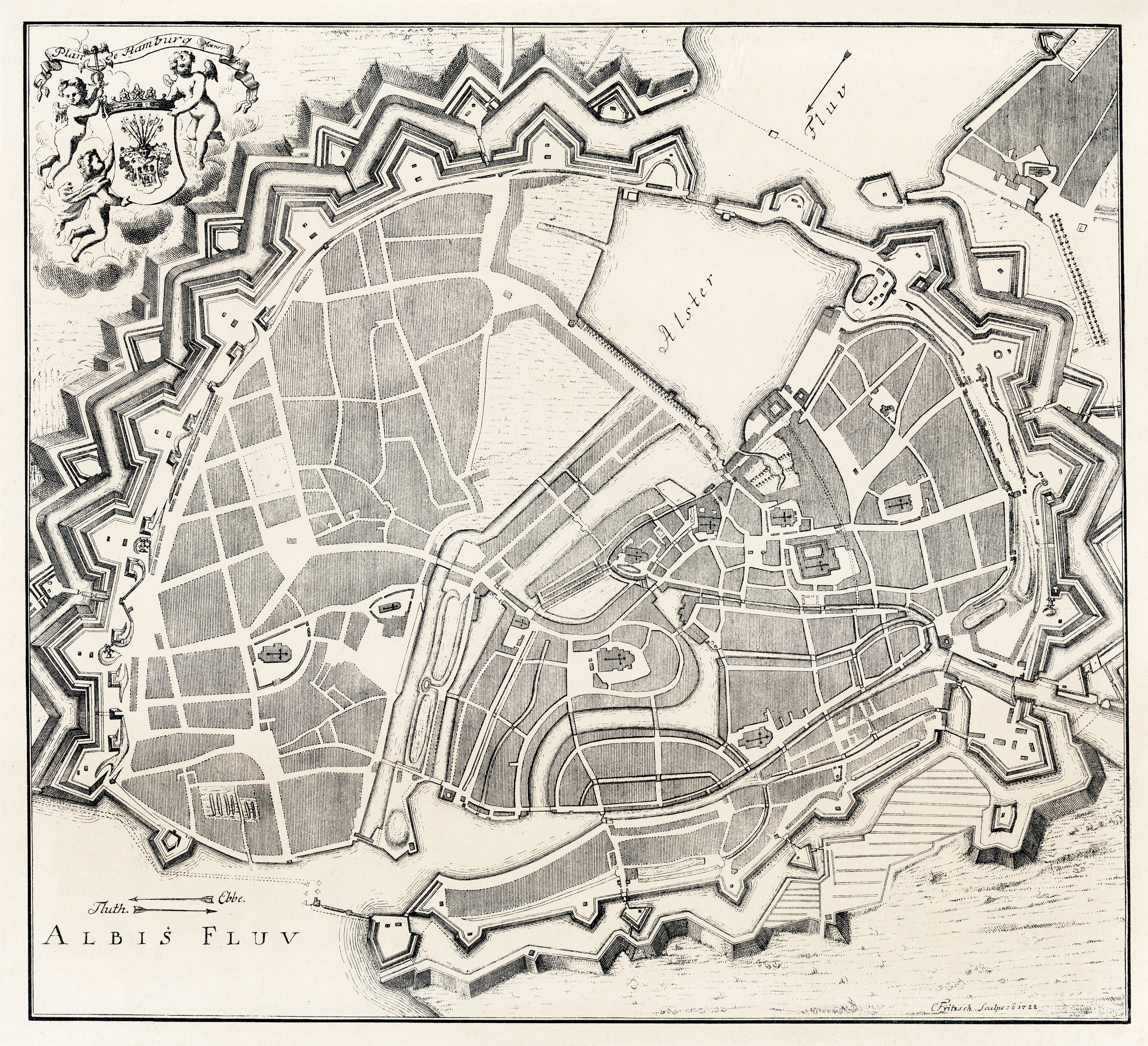
The following sections demonstrate in an exemplary way the transferability of the object extraction workflow described in 4.2 by means of two more historical map subsets illustrating the same spatial extent of the city of Hamburg (hereinafter named as “map A” and “map B”, see Fig. 9a and b, respectively). Minor changes had to be conducted to achieve optimum results for the two different maps.

Alternative input maps by a Sammlung Christian Terstegge (n.d.) and b Harvard Map Collection, Harvard College Library et al. (2008)
6.1 Map A
Rough building structures could be identified when applying the OBIA workflow to the label-less map A, illustrated in Fig. 9a. However, surface-filling geometries were not detected so that single processing steps had to be modified and added. For instance, to detect the conspicuous hatching of building geometries, a simple line detection algorithm was implemented. Water areas could be identified based on their outstanding hatching pattern consisting of isolated dashes. Small gaps were filled and object contours were closed with the help of morphological closing, which avoids expanding the segmented objects (Chiang et al. 2014; Gede et al. 2020). The resulting classified image objects can be seen in Fig. 10a.

Segmentation results by the use of the adjusted workflows for a map A and b map B
6.2 Map B
Due to its monotonous appearance, a straightforward applicability of the workflow described in Sect. 4.2 was not feasible for map B. The dark contours of building objects were extracted by means of thresholding so that their enclosed textures could simply be classified as buildings as well. Also, water areas could be identified by regarding their distinctive texture. Labels were differentiated and classified based on their neighborly relations to buildings and the maps’ background (roads and places), respectively. As can be seen from Fig. 10b, these relations were not unambiguous in each case.
The map objects’ quality highly depends on the map’s complexity. With a greater degree of complexity, OBIA results became less satisfying. Apart from visual overload, further challenges may impede a segmentation of historical maps:
-
Stains, folds, and tears in the maps’ original material,
-
detailed map objects and symbols (e.g., roofs of buildings, trees, or blades of grass),
-
heterogeneous or absent textures, or
-
overlaps between labels and other map features.
7 Potential Future Applications
With the geometries resulting from the workflow described in chapters 4 and 5, valuable analysis and comparison processes concerning urban morphological developments become possible. According to a preceding user study (Schlegel 2019), comparisons between historical and current maps mainly relate to buildings and roads as well as general transformations in the urban structure. Figure 11 shows two potential use cases: Users may select a historical building whilst, in the background, an intersection algorithm finds appropriate current buildings and outputs related information such as its name or area (see Fig. 11a). Alternatively, current road names might be queried. By selecting a historical road section, the current road name may be returned from a database using the intersection area between the bounding box of the former and the corresponding line feature of the latter (see Fig. 11b).

Exemplary use cases: comparing a historical with a a current building and b a current road section by selecting a historical feature. Based on their intersection area, related information is returned from a corresponding database
8 Discussion
For a considerable enhancement of object extraction processes from historical maps, a preceding elimination of labels is advantageous. Based on the results of a text detection tool used in the course of previous research (Schlegel 2021) and assuming that labels run parallel to roads and edges of buildings, we were able to eliminate straight text.
As gray values of labels often do not differ significantly from the ones of adjacent map objects such as contours or textures of buildings, their existence complicates efforts towards the extraction of geometries from a historical map. In the present work, text was separated from features of similar color by thresholding techniques so that a more precise object extraction became feasible. This procedure is irrespective of any preceding map enhancements or georeferencing and efficient especially for monochrome historical maps having a heterogeneous background. In contrast to other studies, our suggested approach neither mistakenly removes other map features nor substitutes original pixel values. Nevertheless, an optimization of the preceding text detection should be undertaken so that all map labels are considered for elimination in future research.
A main purpose of this study was to pave the way for a straightforward comparison of large-scale historical maps with recent counterparts. Vectorized and georeferenced map features allow their analyzability and searchability in the further course. With the help of enhanced object-based image analysis as well as subsequent vector refinement and linking processes, we address this issue within a semi-automated workflow. By applying OBIA approaches, not only spectral, but also textural, shape-dependent, or contextual characteristics of map objects are considered for their identification. Available techniques from image and vector processing contributed to an adequate quality of extracted features and to make a large-scale historical map analyzable and comparable. This is inevitable for investigating urban transformations over time. On the downside, specific software, knowledge, and, in some instances, subjective and individual solutions are required, especially within the object extraction domain. Consequently, a fully automated workflow is not realizable.
A critical view on the results shows that these strongly depend on a maps’ complexity and the quality of the underlying bitmap. All processing steps applied to a bitmap are affected by its color depth, format, and resolution (Gede et al. 2020). Further improvements of the suggested methodology may involve a consideration of additional maps, e.g., showing other cities, and algorithms.
By roughly georeferencing large-scale historical with current maps and putting these on top of one another, a direct comparison of their individual objects is facilitated. We suggest to define georeferencing control points based on the shape and context similarities of map features such as public buildings. It is assumed that these buildings were already classified as such from preceding object extraction. To measure the similarity of objects between a historical and a current dataset, two methodologies are presented. It was found that corresponding geometries of churches have a high similarity as, usually, their shapes remain unchanged over centuries. When comparing these for matching purposes, both maps need to have a similar scale and degree of generalization. However, shape similarities are not invariably unambiguous. Distortions induced by adjusting the geometries’ aspect ratios may lead to biased results. Further similarity measures, such as the geographic context, are therefore necessary. The consideration of the geographic context of objects proved beneficial for a quality control of the control points defined for the final georeferencing. Its outcomes depend on the subjective choice of reference points. Finally, georeferencing current with historical maps does not necessarily improve their accuracy. Depending on the particular application, it must be noted that shapes and lines, distances, or proportions may be distorted. Regarding our objective of comparing historical map content, the presented rough georeferencing proved to be satisfying for potential future applications.
9 Conclusion and Outlook
A major purpose of this study was to present the feasibility of a holistic workflow. Within an end-to-end solution, semi-automated approaches to extract and vectorize features from a large-scale, mainly monochrome, historical map were developed and applied for the purpose of providing knowledge, of analyzability (e.g., in GIS), and comparability. A concluding georeferencing enabled a straightforward comparison to current counterparts and, in the further course, to understand changes within a cityscape over time. A significant contribution could be made by previously eliminating map labels and separating them from other objects to improve their extraction results.
It was shown that a rough georeferencing is sufficient for the juxtaposition of historical and current map objects. With the presented methodologies, an appropriate spatial allocation without distorting map objects was achieved. The present findings confirm that each map has an individual need for adaption, but only minor adjustments are required to apply the suggested approaches to maps having a similar degree of complexity.
Overall, our results make a major contribution to extract valuable information from large-scale historical maps by combining approaches for text detection (see Schlegel (2021)), the elimination of labels, OBIA, raster-to-vector conversions, and an approximate spatial referencing based on similarity measures. We thereby provide a starting point for gaining new insights from large-scale historical maps. It should be emphasized that this research serves as a demonstration of a feasible holistic workflow paving the way for the analyzability of large-scale historical maps as well as for their comparison to current counterparts. This was implemented by means of an initial example case. In terms of future research, it would be useful to extend the current findings by examining additional maps. Also, further considerations should include the practicability of comparison analyses as illustrated exemplarily in chapter 7.
Code Availability
All source code and exemplary data sets are openly available for reproducibility at https://github.com/IngaSchl/Object-Extraction.
References
Ablameyko S, Bereishik V, Homenko M, Lagunovsky D, Paramonova N, Patsko O (2002) A complete system for interpretation of color maps. IJIG 2(3):453–479. https://doi.org/10.1142/S0219467802000767
Ahmad J, Sajjad M, Mehmood I, Rho S, Baik SW (2014) Describing colors, textures and shapes for content based image retrieval: a survey. J Platform Tech 2(4):34–48
Arteaga MG (2013) Historical map polygon and feature extractor. In: Proceedings of the 1st ACM SIGSPATIAL International Workshop on MapInteraction. Association for Computing Machinery, New York, NY, pp 66–71. https://doi.org/10.1145/2534931.2534932
Behörde für Verkehr und Mobilitätswende (BVM) (2020) Straßen- und Wegenetz Hamburg (HH-SIB): “WFS Straßen- und Wegenetz Hamburg” (GetCapabilities). Transparenzportal Hamburg. https://suche.transparenz.hamburg.de/dataset/strassen-und-wegenetz-hamburg-hh-sib16?forceWeb=true. Accessed 16 May 2022
Bertalmío M, Bertozzi AL, Sapiro G (2001) Navier-Stokes, fluid dynamics, and image and video inpainting. In: Proceedings of the 2001 IEEE Computer Society Conference on Computer Vision and Pattern Recognition, pp I-I. https://doi.org/10.1109/CVPR.2001.990497
Bhowmik S, Sarkar R, Nasipuri M, Doermann D (2018) Text and non-text separation in offline document images: a survey. IJDAR 21:1–20. https://doi.org/10.1007/s10032-018-0296-z
Blaschke T, Hay GJ, Kelly M, Lang S, Hofmann P, Addink E, Queiroz Feitosa R, van der Meer F, van der Werff H, van Coillie F, Tiede D (2014) Geographic object-based image analysis – towards a new paradigm. ISPRS J Photogramm Remote Sens 87(100):180–191. https://doi.org/10.1016/j.isprsjprs.2013.09.014
Brown KD (2002) Raster to vector conversion of geologic maps: using R2V from able software corporation. In: Soller DR (ed) Digital Mapping Techniques ’02 – Workshop Proceedings, pp 203–205
Chaves M (2021, January) GLCMs – a Great Tool for Your ML Arsenal. Towards Data Science. https://towardsdatascience.com/glcms-a-great-tool-for-your-ml-arsenal-7a59f1e45b65. Accessed 23 June 2022
Chiang YY (2017) Unlocking textual content from historical maps - potentials and applications, trends, and outlooks. recent trends in image processing and pattern recognition. RTIP2R 2016. Commun Comput Info Sci 709:111–124. https://doi.org/10.1007/978-981-10-4859-3_11
Chiang YY, Knoblock CA (2012) Generating named road vector data from raster maps. In: Xiao N, Kwan MP, Goodchild MF, Shekhar S (eds) Geographic Information Science. GIScience 2012: Lecture Notes in Computer Science 7478. Springer, Berlin, Heidelberg, pp 57–71
Chiang YY, Knoblock CA (2013) A general approach for extracting road vector data from raster maps. IJDAR 16:55–81. https://doi.org/10.1007/s10032-011-0177-1
Chiang YY, Knoblock CA (2014) Recognizing text in raster maps. GeoInformatica 19(1):1–27. https://doi.org/10.1007/s10707-014-0203-9
Chiang YY, Leyk S, Knoblock CA (2011) Efficient and robust graphics recognition from historical maps. In: Kwon YB, Ogier JM (eds) Graphics recognition: new trends and challenges: Lecture Notes in Computer Science 7423. Springer, Berlin, Heidelberg, pp 25–35
Chiang YY, Leyk S, Knoblock CA (2014) A survey of digital map processing techniques. ACM Comput Surv 47(1):1–44. https://doi.org/10.1145/2557423
Chiang YY, Duan W, Leyk S, Uhl JH, Knoblock CA (2020) Using historical maps in scientific studies: applications, challenges, and best practices. Springer, Cham
Chrysovalantis DG, Nikolaos T (2020) Building footprint extraction from historic maps utilizing automatic vectorisation methods in open source GIS software. In: Krisztina I (ed) Automatic vectorisation of historical maps. Department of Cartography and Geoinformatics, ELTE Eötvös Loránd University, Budapest, pp 9–17
Clark B, MacFadyen J (2020, Oct 7) ArcGIS Pro Lesson 2: Georeferencing Historical Maps. Geospatial Historian. https://geospatialhistorian.wordpress.com/arcgis-pro-lesson-2-georeferencing-maps/#Step4. Accessed 02 June 2022
Claussen JH (n.d.) Die Geschichte von St. Nikolai – Teil 3. https://www.mahnmal-st-nikolai.de/?page_id=344. Accessed 30 June 2022
Dalang O (2019) VectorBender (Version 0.1.1). https://github.com/olivierdalang/VectorBender. Accessed 02 June 2022
Dornik A, Drǎguţ L, Urdea P (2016) Knowledge-based soil type classification using terrain segmentation. Soil Res 54(7):809–823. https://doi.org/10.1071/SR15210
Edler D, Bestgen A, Kuchinke L, Dickmann F (2014) Grids in topographic maps reduce distortions in the recall of learned object locations. PLoS ONE. https://doi.org/10.1371/journal.pone.0098148
Esri (2022) Envelope. http://esri.github.io/geometry-api-java/doc/Envelope.html. Accessed 01 June 2022
Frank R, Ester M (2006) A quantitative similarity measure for maps. In: Riedl A, Kainz W, Elmes GA (eds) Progress in spatial data handling. Springer, Berlin, Heidelberg, pp 435–450. https://doi.org/10.1007/3-540-35589-8_28
Gede M, Árvai V, Vassányi G, Supka Z, Szabó E, Bordács A, Varga CG, Irás K (2020) Automatic vectorisation of old maps using QGIS – tools, possibilities and challenges. In: Krisztina I (ed) Automatic vectorisation of historical maps. ELTE Eötvös Loránd University, Budapest, Department of Cartography and Geoinformatics, pp 37–43
Gobbi S, Ciolli M, La Porta N, Rocchini D, Tattoni C, Zatelli P (2019) New tools for the classification and filtering of historical maps. IJGI 8(10):455. https://doi.org/10.3390/ijgi8100455
Godfrey B, Eveleth H (2015) An adaptable approach for generating vector features from scanned historical thematic maps using image enhancement and remote sensing techniques in a geographic information system. J Map Geogr Libraries 11(1):18–36. https://doi.org/10.1080/15420353.2014.1001107
Harvard Map Collection, Harvard College Library, Lindley W, engineer, Society for the Diffusion of Useful Knowledge (Great Britain), Cox G, publisher, Davies BR (n.d.) Hamburg, Germany, 1853 (Raster Image). Princeton University Library. https://maps.princeton.edu/catalog/harvard-g6299-h3-1853-l5. Accessed 26 Apr 2019
Harvard Map Collection, Harvard College Library, Mirbeck CLB, Baker B (2008) Hamburg, Germany, 1803 (Raster Image): Web Map Service (WMS). Harvard Geospatial Library. https://hgl.harvard.edu/catalog/harvard-g6299-h3-1803-m5. Accessed 31 May 2018
Havlicek J, Cajthaml J (2014) The influence of the distribution of ground control points on georeferencing. In: Proceedings of the 14th International Multidisciplinary Scientific Geoconference SGEM vol. III, 965972
Hay GJ, Castilla G (2008) Geographic Object-Based Image Analysis (GEOBIA): a new name for a new discipline. In: Blaschke T, Lang S, Hay GJ (eds) Object-based image analysis: spatial concepts for knowledge-driven remote sensing applications. Springer, Berlin, Heidelberg, pp 75–110
Heitzler M, Hurni L (2020) Cartographic reconstruction of building footprints from historical maps: a study on the Swiss Siegfried map. Trans GIS 24(2):442–461. https://doi.org/10.1111/tgis.12610
Herold H (2018) Geoinformation from the past: computational retrieval and retrospective monitoring of historical land use. Springer, Wiesbaden
Herrault PA, Sheeren D, Fauvel M, Paegelow M (2013) Automatic extraction of forests from historical maps based on unsupervised classification in the CIELab Color Space. In: Vandenbroucke D, Bucher B, Crompvoets J (eds) Geographic information science at the heart of Europe: Lecture Notes in Geoinformation and Cartography. Springer, Cham, pp 95–112
Hussain M, Chen D, Cheng A, Wei H, Stanley D (2013) Change detection from remotely sensed images: From pixel-based to object-based approaches. ISPRS J Photogramm Remote Sens 80:91–106. https://doi.org/10.1016/j.isprsjprs.2013.03.006
Iosifescu I, Tsorlini A, Hurni L (2016) Towards a comprehensive methodology for automatic vectorization of raster historical maps. e-Perimetron 11(2):57–76
Jiao C, Heitzler M, Hurni L (2020) Extracting wetlands from Swiss historical maps with convolutional neural networks. In: Krisztina I (ed) Automatic vectorisation of historical maps. ELTE Eötvös Loránd University, Budapest, Department of Cartography and Geoinformatics, pp 31–36
Kaur D, Kaur Y (2014) Various image segmentation techniques: a review. IJCSMC 3(5):809–814
Kerle N, de Leeuw J (2009) Reviving legacy population maps with object-oriented image processing techniques. IEEE Trans Geosci Remote Sens 47(7):2392–2402. https://doi.org/10.1109/TGRS.2008.2010853
Kim JO, Yu K, Heo J, Lee WH (2010) A new method for matching objects in two different geospatial datasets based on the geographic context. CAGEO 36(9):1115–1122. https://doi.org/10.1016/j.cageo.2010.04.003
Kim NW, Lee J, Lee H, Seo J (2014) Accurate segmentation of land regions in historical cadastral maps. J vis Commun Image Represent 25(5):1262–1274. https://doi.org/10.1016/j.jvcir.2014.01.001
Landesbetrieb Geoinformation und Vermessung (2022) ALKIS - ausgewählte Daten Hamburg: 2018–01 (GML, 526 MB). Transparenzportal Hamburg. https://daten-hamburg.de/geographie_geologie_geobasisdaten/ALKIS_Liegenschaftskarte/ALKIS_Liegenschaftskarte_ausgewaehlteDaten_HH_2018-01-06.zip. Accessed 18 May 2022
Laycock SD, Brown PG, Laycock RG, Day AM (2011) Aligning archive maps and extracting footprints for analysis of historic urban environments. Comput Graph 35(2):242–249. https://doi.org/10.1016/j.cag.2011.01.002
Le Riche M (2020) Identifying Building Footprints in Historic Map Data using OpenCV and PostGIS. In: Krisztina I (ed) Automatic Vectorisation of Historical Maps. ELTE Eötvös Loránd University, Budapest, Department of Cartography and Geoinformatics, pp 18–30
Leyk S, Boesch R (2010) Colors of the past: Color image segmentation in historical topographic maps based on homogeneity. GeoInformatica 14(1):1–21. https://doi.org/10.1007/s10707-008-0074-z
Leyk S, Boesch R, Weibel R (2006) Saliency and semantic processing: extracting forest cover from historical topographic maps. Pattern Recogn 39(5):953–968. https://doi.org/10.1016/j.patcog.2005.10.018
Li Z, Chiang YY, Banisetti S, Kejriwal L (2018) strabo-text-recognition-deep-learning (Version 0.67). https://github.com/spatial-computing/strabo-text-recognition-deep-learning. Accessed 04 Nov 2020
Loran C, Haegi S, Ginzler C (2018) Comparing historical and contemporary maps - a methodological framework for a cartographic map comparison applied to Swiss maps. IJGIS 32(11):2123–2139. https://doi.org/10.1080/13658816.2018.1482553
MacEachren AM (1985) Compactness of geographic shape: comparison and evaluation of measures. Geografiska Annaler Series b: Hum Geogr 67(1):53–67. https://doi.org/10.1080/04353684.1985.11879515. (Taylor & Francis, Ltd)
Muhs S, Herold H, Meinel G, Burghardt D, Kretschmer O (2016) Automatic delineation of built-up area at urban block level from topographic maps. Comput Environ Urban Syst 58:71–84. https://doi.org/10.1016/j.compenvurbsys.2016.04.001
Neubert M. (2005) Bewertung, Verarbeitung und segmentbasierte Auswertung sehr hoch auflösender Satellitenbilddaten vor dem Hintergrund landschaftsplanerischer und landschaftsökologischer Anwendungen. Dissertation, Technische Universität Dresden
Ostafin K, Iwanowski M, Kozak J, Cacko A, Gimmi U, Kaim D, Psomas A, Ginzler C, Ostapowicz K (2017) Forest cover mask from historical topographic maps based on image processing. Geosci Data J 4(1):29–39. https://doi.org/10.1002/gdj3.46
Pearson M, Mohammed GS, Sanchez-Silva R, Carbajales P (2013) Stanford University libraries study: topographical map vectorization and the impact of Bayer Moiré Defect. J Map Geogr Libraries 9(3):313–334. https://doi.org/10.1080/15420353.2013.820677
Peller P (2018) From paper map to geospatial vector layer: demystifying the process. IASSIST Q 42(3):1–24
Rumsey D, Williams M (2002) Historical maps in GIS. In: Knowles AK (ed) Past time, past place: GIS for history. Esri Press, Redlands, CA, pp 1–18
Samal A, Seth S, Cueto K (2004) A feature-based approach to conflation of geospatial sources. IJGIS 18(5):459–489. https://doi.org/10.1080/13658810410001658076
Sammlung Christian Terstegge (n.d.) 1722, von C. Fritzsch, photo-lithographisches Replikat vom Verlag Strumper & Co., 1880. https://www.christian-terstegge.de/hamburg/karten_hamburg/files/1722_fritzsch_strumper_300dpi.jpeg. Accessed 4 Feb 2022
Schlegel I (2019) Empirical study for a deployment of a methodology for improving the comparability between historical and current maps. KN - J Cartogr Geogr Info 69(2):121–130. https://doi.org/10.1007/s42489-019-00016-0
Schlegel I (2021) Automated extraction of labels from large-scale historical maps. AGILE GIScience Series. https://doi.org/10.5194/agile-giss-2-12-2021
Skopyk B (2021, March 8) Georeferencing Historical Maps: Methods, best practices, and a tutorial in ArcGIS Pro. ArcGIS StoryMaps. https://storymaps.arcgis.com/stories/dd75d0398f7d4ded924d303161895b8b. Accessed 30 June 2022
Stefanidis A, Agouris P, Georgiadis C, Bertolotto M, Carswell JD (2002) Scale- and orientation-invariant scene similarity metrics for image queries. IJGIS 16(8):749–772. https://doi.org/10.1080/13658810210148552
Sun K, Hu Y, Song J, Zhu Y (2021) Aligning geographic entities from historical maps for building knowledge graphs. IJGIS 35(10):2078–2107
Tang W, Hao Y, Zhao Y, Li N (2008) Feature matching algorithm based on spatial similarity. In: Proceedings of SPIE 7147, Geoinformatics 2008 and Joint Conference on GIS and Built Environment: Classification of Remote Sensing Images, 714704. https://doi.org/10.1117/12.813204
Telea A (2004) An image inpainting technique based on the fast marching method. JGT 9(1):25–36. https://doi.org/10.1080/10867651.2004.10487596
Trimble Inc. (2021) Haralick texture. https://docs.ecognition.com/v10.0.2/#eCognition_documentation/Reference Book/03 Features/2 Object features/4 Texture/Haralick texture.htm?Highlight=haralick. Accessed 25 May 2022
Trimble Inc. (2022) The Power of eCognition. https://docs.ecognition.com/#eCognition_documentation/Modules/1 eCognition at a glance/01 Introduction to the Power of eCognition.htm. Accessed 24 May 2022
Uhl JH, Leyk S, Chiang YY, Duan W, Knoblock CA (2017) Extracting Human Settlement Footprint from Historical Topographic Map Series Using Context-Based Machine Learning. In: Proceedings of the 8th International Conference of Pattern Recognition Systems. https://doi.org/10.1049/cp.2017.0144
Xavier EMA, Ariza-López FJ, Ureña-Cámara MA (2016) A survey of measures and methods for matching geospatial vector datasets. ACM Comput Surv 49(2):1–34. https://doi.org/10.1145/2963147
Xydas C, Kesidis A, Kalogeropoulos K, Tsatsaris A (2022) Buildings Extraction from Historical Topographic Maps via a Deep Convolution Neural Network. In: Proceedings of the 17th International Joint Conference on Computer Vision, Imaging and Computer Graphics Theory and Applications 5, pp 485–492. https://doi.org/10.5220/0010839700003124
Zatelli P, Gobbi S, Tattoni C, La Porta N, Ciolli M (2019) Object-based image analysis for historic maps classification. Int Arch Photogramm Remote Sens Spat Inf Sci XLII-4/W14:247–254
Funding
Open Access funding enabled and organized by Projekt DEAL. No funds, grants, or other support was received.
Author information
Authors and Affiliations
Corresponding author
Ethics declarations
Conflict of Interest
The authors report there are no competing interests to declare.
Rights and permissions
Open Access This article is licensed under a Creative Commons Attribution 4.0 International License, which permits use, sharing, adaptation, distribution and reproduction in any medium or format, as long as you give appropriate credit to the original author(s) and the source, provide a link to the Creative Commons licence, and indicate if changes were made. The images or other third party material in this article are included in the article's Creative Commons licence, unless indicated otherwise in a credit line to the material. If material is not included in the article's Creative Commons licence and your intended use is not permitted by statutory regulation or exceeds the permitted use, you will need to obtain permission directly from the copyright holder. To view a copy of this licence, visit http://creativecommons.org/licenses/by/4.0/.
About this article

Cite this article
Schlegel, I. A Holistic Workflow for Semi-automated Object Extraction from Large-Scale Historical Maps. KN J. Cartogr. Geogr. Inf. 73, 3–18 (2023). https://doi.org/10.1007/s42489-023-00131-z
Received:
Accepted:
Published:
Issue Date:
DOI: https://doi.org/10.1007/s42489-023-00131-z
Keywords
- Historical maps
- Object extraction
- Object-based image analysis (OBIA)
- Map comparison
- Vectorization
- Georeferencing