
Abstract
China vigorously implements the dual carbon strategy, and natural gas consumption continues to grow rapidly. It is urgent to improve the natural gas “production, supply, storage, and sales” system and accelerate the construction of underground gas storage (UGS). UGS requires “storage, injection, and extraction”. Faults are the primary factor of “storage”, the evaluation of fault-sealing is crucial for the safe construction and operation of UGS. Existing researches start from the perspective of the hydrocarbon reservoir, develop an evaluation of the basic characteristics of faults, lithological configuration of the fault’s two blocks, analysis of production performance, Shale Smear Factor (SSF), Shale Gouge Ratio (SGR), properties of fault-filling materials, 3D tectonic model, normal pressure on the fault plane, fault shear index, and fault plugging coefficient. This paper systematically analyzes the adaptability of existing methods and proposes an index to evaluate the fault-sealing capability of UGS. Taking the first UGS in SW China—Xiangguosi UGS as a case, using this workflow to evaluate the fault-sealing capability of 5 major faults. It is believed that the evaluation of fault-sealing on Xiangguosi UGS is good. This conclusion supports the design of construction key indicators and is the important basis point of the construction of the “signpost” UGS. It is of guiding significance and provides a reference for the evaluation of fault-sealing for the rebuilding of depleted gas reservoirs to UGSs.
1 Introduction
Faults serve as active migration pathways during reservoir formation or shielding conditions for hydrocarbon accumulation [1,2,3,4]. Fault-sealing refers to a sort of identity for both the upper block and the lower block of fault planes or faulted zones together with these two blocks to obstruct formation fluids and prevent fluid flow owing to the difference in displacement pressure. As a fundamental element to affect fault block traps to form reservoirs and reservoir-forming size, the sealing may be employed to estimate the size of fault block reservoirs, the fullness of hydrocarbon, and the natural gas capacity of a UGS. It is also the defense for the safe running of a UGS [5,6,7,8]. Since Lindsay et al. [9] proposed the algorithm of Shale Smear Factor (SSF) in 1993, Yielding et al. [10] proposed the algorithm of Shale Gouge Ratio (SGR) in 2002, the quantitative evaluation of fault-sealing is becoming a standard workflow. The mechanical stability evaluation is also not to be outdone. Chen [11] proposed the algorithm of normal pressure on the fault plane in 1987, Liu [5] proposed the algorithm of fault plugging coefficient in 1998, and Wang and Dai [12] improved the algorithm of fault shear index in 2012. But those researchers don’t summarize the evaluation methods of fault-sealing, usually 1 to 2 aspects or 2 to 3 aspects, for example, Fu et al. [13] in 2021. This paper summarizes the existing experience, systematically analyzes the adaptability of existing methods, and proposes an index to evaluate the fault-sealing capability of UGS. The methods start from three aspects of qualitative, quantitative, and mechanical stability evaluation based on the basic characteristics of faults, lithological configuration of the fault’s two blocks, analysis of production performance, Shale Smear Factor (SSF), Shale Gouge Ratio (SGR), properties of fault-filling materials, 3D tectonic model, normal pressure on the fault plane, fault shear index, and fault plugging coefficient, could provide a very complete and comprehensive evaluation of fault-sealing.
Xiangguosi UGS is the first UGS in SW China, which is built from the Carboniferous depleted gas reservoir in Xiangguosi structure with highly steep strata and well-developed faults (Fig. 1). The reservoir is treated as both injection and production targets [14]. The geologic reserve is 43.9 × 10⁸ m3, with accumulated gas production of 40.24 × 10⁸ m3. It has been operating efficiently for 10 years, with a total of 158 × 108 m3 gas injection and 128 × 108 m3 gas production. Xiangguosi UGS fulfills 17% of the actual peak-adjustment and supply guarantee tasks with 13% of the designed gas storage capacity in China, is of vital importance, and is an indispensable assistance for China to achieve carbon neutrality before 2060. Combining qualitative, quantitative, and mechanical stability evaluation, using this workflow to evaluate the fault-sealing capability of 5 major faults. It is believed that the evaluation of fault-sealing on Xiangguosi UGS is good. This conclusion supporting the design of construction key indicators and the first demonstration of “Expand the pressure range, increase the production” in China, is the important basis point of the construction of the “signpost” UGS. It is of guiding significance and provides a reference for the evaluation of fault-sealing for the rebuilding of depleted gas reservoirs to UGSs.

The location diagram of Xiangguosi UGS. Both images in Figure 1 were downloaded from the official website of the Ministry of Natural Resources of China
2 Regional background of Xiangguosi UGS
2.1 Geological setting of Xiangguosi UGS
Xiangguosi UGS is the first UGS in SW China, stretches across over Yubei and Beibei districts, Chongqing City, covering an exploration area of 447.81 km2. The study area is characterized by mountainous terrain with significant terrain fluctuations, with a minimum elevation of 200 m and a maximum elevation of 1040 m, with a relative elevation difference of 840 m. The central part of the study area has steep mountains, crisscrossed gullies, and severely cut terrain. Most areas on both sides are relatively flat. Regionally, it is subordinate to one local structure in the southern end of the Huaying Mountain tectonic group, a middle-uplift high-steep area in the southeastern Sichuan Basin. The tectonic strike is NNE.
No fault is found on the ground in the Xiangguosi structure while increasing folding inside the hinterland where a great deal of reverse faults is developed with various throws. Accompanying high structural, major faults are often extended over the leading portion of the Xiangguosi structure with a long strike length and straddle the whole study area. They twist with the structure along tectonic trends to control structural shape and scale. There are 92 reverse faults. From west to east, fault ①, fault ⑤, fault ②, fault ④, and fault ③ are major faults with larger sizes (Fig. 2), whose throw is more than that of others. Fault ①, fault ⑤, and fault ② in the northwestern flank die out upwards in Xujiahe Formation and downwards in Silurian System while fault ④ and fault ③ in the southeastern flank die out upwards in Jialingjiang Formation and downwards in Silurian System.

The reflection structure diagram of lower Permian of Xiangguosi UGS
2.2 Stratigraphic and sedimentary characteristics of Xiangguosi UGS
The Silurian in this study area is dominated by coastal and neritic clastic and carbonate rocks with a thickness of 400–1 200 m. Among these, with a thickness of 229–299 m, Longmaxi Formation along the Huaying Mountain possesses growing sandy-argillaceous content. The Lower Devonian System is made up of clastic rocks. The Middle Devonian System is made up of carbonate and clastic rocks. The Upper Devonian System is made up of carbonate rocks. The Lower Carboniferous System is made up of carbonate rocks interbedded with a little purple-red sandstone, mudstone, and hematite. The Upper Carboniferous System is made up of entire carbonate rocks. The Lower Permian System is made up of clastic rocks and limestone. The Upper Permian System is made up of limestone and siliceous rock interbedded with limestone. The Lower Triassic System is made up of clastic rocks, which are in decline whereas carbonate rocks are increasing, occasionally interbedded with mud shale rocks (Fig. 3).

The stratigraphic columnar profile of Xiangguosi UGS
3 Fault qualitative evaluation
3.1 Basic characteristics of fault
3.1.1 Fault activities
According to the length of the fault activity period, faults are divided into short-term active faults and long-term active faults. Short-term active faults can be divided into early-stage, simultaneous-stage, and late-stage in accordance with the relevance to large-scale hydrocarbon migration and accumulation periods [15]. Long-term ones possess moderate fault-sealing [16]. After contrasting the proportion of forming reservoirs with regard to the quantity of fault-controlled structures, it is concluded best sealing in early-stage among short-term active faults of all kinds, followed by simultaneous and late ones [17].
3.1.2 Fault mechanical properties
According to mechanical properties, faults are divided into wrench faults, extensional faults, and compressional faults. Strike-slip faults are the products of wrench faults. During the process of displacement, the rock on both blocks of the fault is relatively displaced over a long distance, with close friction and grinding, usually developed into a range of fault gouge on fault planes, which is conducive to hydrocarbon closure. The proportion of fault breccia is high in extensional fault zones, which brings about poor sealing [18]. The fault-sealing in compressional faults is between wrench faults and extensional faults.
3.1.3 Fault geometry
Occurrence is made up of three elements, strike, dip, and dip angle. Among these, strike exerts a significant influence on fault-sealing (fault-sealing coefficient, If). The greater the angle between strike and tectonic stress (φ) is, the better the fault-sealing is, while the smaller the angle is, the poorer the sealing is. For example, when the differential stress is on line c, 10 MPa, φA = 30°, φB = 60°, IfB is bigger than IfA, which means the fault-sealing of B is bigger than the fault-sealing of A (Fig. 4).

The relationship diagram of fault-sealing and strike
Differential stress in a, b, c, d, and e solid lines is 0 MPa, 5 MPa, 10 MPa, 15 MPa, and 20 MPa, respectively. Pressure (σti) is 0, abnormal pressure coefficient (f) is 1.0, Poisson’s ratio (μ) is 0.3, dip angle (θ) is 60°, and depth (h) is 2,000 m. Differential stress in a’, b’, c’, d’, and e’ dashed lines is 0 MPa, 5 MPa, 10 MPa, 15 MPa, and 20 MPa, respectively. The abnormal pressure coefficient (f) is 1.5 and the others are the same as above [19].
The dip angle (θ) has an impact on the fault-sealing as well. The smaller the dip angle is, the better the sealing is in extensional basins, while the bigger the angle is, the better the sealing in compressional basins, and the fault-sealing in torsion basins is between extensional basins and compressive basins [19]. In extensional basins, at the same depth, the stress is generally between 5 and 20 MPa (the orange area). In compressional basins, at the depth of 3000 m, the maximum principal compressive stress can be 150 MPa, and the average principal compressive stress can also reach 100 MPa (the green area). For example, in an extensional basin, when the stress is 15 MPa, φA = 30°, φA’ = 60°, IfA is bigger than IfA’, which means the fault-sealing of A is bigger than the fault-sealing of A’. In a compressional basin, when the stress is 110 MPa, φB = 45°, φB’ = 30°, IfB is bigger than IfB’, which means the fault-sealing of B is bigger than the fault-sealing of B’ (Fig. 5).

The relationship diagram of fault-sealing and the dip angle
Dip angle in a, b, c, d, and e solid lines is 0°,30°,45°,60°, and 90°, respectively. φ is 90°, f is 1.0, μ is 0.3, and h is 3000 m. Dip angle in a’, b’, c’, d’, and e’ dashed lines is 0°, 30°, 45°, 60°, and 90°, respectively. The abnormal pressure coefficient (f) is 1.6 and the others are the same as above [19].
3.2 Lithological configuration relationship between two blocks
Fault blocks are rocks that displace along both sides of the fault plane. The upper block is located on the upper side of the fault plane, and the lower block is located on the lower side of the fault plane. The lithological configuration relationship between two blocks is one of the critical conditions to judge one fault with or without sealing identity. And this configuration is also exactly regarded as the principle to study the typical fault-sealing [20, 21]. It is generally accepted that fine sealing in one configuration on the target block of sandstone with the opposite of mudstone while poor in the other configuration of sandstone with sandstone, which is dependent on the discrepancy between one displacement pressure to close off sandstone and the other in reservoir stratum [5]. Zhao et al. [22] divided the configuration into 12 modes. The fault plane in the first mode is a single fault plane without any blocking effect on hydrocarbon. While faulted zone in the second mode is likely to close off hydrocarbon (Fig. 6).

The sketch diagram of lithological configuration relationship between two blocks
Plower reservoir stands for the displacement pressure of the reservoir stratum on the lower block. Pupper reservoir stands for the displacement pressure of the reservoir stratum on the upper block. Pupper mudstone stands for the displacement pressure of the mudstone stratum on the upper block. PF1 stands for the displacement pressure in the first fault zone, and PF2 stands for the displacement pressure in the second fault zone.
Drawing the Allan figure is the most powerful method to study the lithological configuration relationship [21, 23]. The Allan figure is made of seismic profiles and tectonic diagrams. The whole drawing procedure includes (i) selecting an appropriate survey line, (ii) recording the time value at every breaking point, (iii) conversion of the time domain and depth domain, (iv) projecting the strata in contact with the fault plane on both blocks of the fault, and (v) obtaining the lithological configuration relationship of the two blocks by ways of variations of fault throw. Eventually, the configuration on both sides of the fault plane can be received intuitively [24,25,26].
3.3 Analysis of fault production performance
Fault production performance data can reflect the sealing feature in reservoirs [16]. Analyzing the pressure, oil–water distribution of wells in two blocks of the fault, and other performance data can understand the fault-sealing more specifically [27]. When the production capacity of an oil well declines at one side of the fault, water injection could be implemented into the same stratum on the other side. As shown in Fig. 4a, this fault is connected if oil production is increasing and there are no other water injection wells. As shown in Fig. 4b, this fault is connected if the polymer is found at the same stratum in this oil well after the polymer is added to the water injection well, or if this fault is sealed (Fig. 7).

The sketch diagram of stratigraphic communication on both sides of the fault [28]
4 Fault quantitative evaluation
4.1 Shale smear factor (SSF)
The shale smear factor is a parameter to characterize the extensive continuity of shale smear layers, reflecting the growth level of the shale smear. And it is an essential factor to evaluate effective fault-sealing [9]. The smaller the SSF is, the better the smear continuity and the fault-sealing are. The equation is as follows:
D stands for the vertical fault throw, m; and di stands for the shale thickness in the ith layer within the vertical fault throw, m.
4.2 Shale gouge ratio (SGR)
The shale gouge ratio is a parameter to characterize the percentage of clay minerals in the gouge of fault zones [10], it can show the shale content in layers in the most effective way [29], and it is a considerable parameter for quantitatively revealing the fault-sealing [27]. In fault zones, the higher the SGR is, the larger the displacement pressure needed for formation fluids to break through this fault, the better the fault-sealing is. To this end, a large amount of hydrocarbon can be gathered around reservoir strata to form hydrocarbon reservoirs [16]. The equation is as follows:
hi stands for the formation thickness in the ith layer. m; Vi stands for the percentage of argillaceous thickness to formation thickness in the ith layer; D stands for the vertical fault throw, m (Figs. 8, 9).
It is well known that if SSF < 4, SGR > 20%, the fault has sealing property [13]

The algorithm diagram of SSF ([10], revised)

The algorithm diagram of SGR ([10], revised)
4.3 Properties of fault-filling material
If the fault-filling material is mainly argillaceous, small particle size and soft hardness may lead to compression and diagenesis under overburden pressure, compactness grows stronger with porosity and permeability decrease owing to this [30]. In addition, mudstone is prone to plastic flow under overburden pressure to stop leaking voids and make the sealing more powerful [31]. If the fault-filling material is mainly sandy, compactness weakens as well as porosity and permeability get better, which creates poor sealing [32]. The equation is as follows:
h stands for the cumulative mean thickness of target mudstone across two blocks, and it can be an average value of cumulative thickness of mudstone in apart wells deployed on both sides; H stands for the fault formation thickness, m; D stands for the vertical fault throw, m; n1 and n2 are the number of mudstone strata offset by two blocks; h1i and h2j are mudstone thickness in the ith and the jth layers of both upper block and lower block, m (Fig. 10).
Rm not only considers the lithology and fault throw of the target layer but also takes into account the lithological characteristics of the strata between the two target layers, which can reflect the size of the mud content in the fault-filling material. Fault-sealing is thought to be poor at Rm below 0.3, moderate at Rm between 0.3 and 0.6, and good at Rm above 0.6

The algorithm diagram of Rm
5 Fault mechanical stability evaluation
5.1 3D tectonic model
Accurate 3D tectonic models are achieved through Petrel. 3D tectonic models are built on well location, well deviation, stratigraphic, well-logging data. While building models, both prompt amendments and adjustments should be done in accordance with tectonic features. Consequently, the tectonic models match seismic data and geological rules [33] for more precise analysis.
5.2 Normal pressure on the fault plane
The stress of faults comes from normal pressure on the fault plane exerted by overburden gravitation [34]. The equation is as follows:
P stands for the normal pressure on the fault plane, P1 and P2 are the horizontal and vertical components of P, MPa; H stands for the burial depth of the fault plane, m; \({\rho }_{r}\) stands for the average overburden density, g/cm3; \({\rho }_{w}\) stands for the density of formation water, g/cm3; θ stands for the dip angle of the fault plane, °. \({\rho }_{r}\) can be obtained from well-logging data or the relationship curve of actual formation density and burial depth. H and θ can be obtained from seismic data [35] (Fig. 11).

The sketch diagram of stress on the fault plane
Consistent with the above equation, P stands for the normal pressure on the fault plane, P1, and P2 are the horizontal and vertical components of P, MPa; H stands for the burial depth of the fault plane, m; θ stands for the dip angle of the fault plane, ° [36].
The normal pressure on the fault plane is one of the influential factors in the capability of vertical fault-sealing. Since it not only makes the fault plane enclosed but also decides gypsum and mudstone deformation inside fault zones [37]. Deformed mudstone fills with fractures in fault zones when the normal pressure is higher than the deformation intensity in mudstone, leading to vertical fault-sealing. Otherwise, faults are vertically open [11]. From some previous experiments on compression resistance to argillaceous rocks in Hunan and Hubei Provinces, it is suggested that the critical pressure of 5 MPa. However, there are differences in mechanical properties in mudstone developed at various areas or layers. Thus, it is essential to redetermine this property in practice [30].
5.3 Fault shear index
The fault shear index is the ratio of shear stress to material shear strength on the fault plane in the fault zones. The equation is as follows:
τ stands for the shear stress on the fault plane; σC stands for the material shear strength in the fault zone; C stands for the intrinsic shear intensity; ω stands for the internal friction coefficient; σ stands for the normal pressure on the fault plane.
In the quantitative evaluation of fault sealing, obtaining the stress value of the fault plane is the key to solving the problem. In general, the fault shear index depends upon the regional in-situ stress field. At present, the most intuitive and accurate method to obtain stress values is to conduct on-site stress testing. But this often encounters many difficulties that are difficult to solve. The in-situ stress can still be measured through hydraulic fracturing, acoustic emission, and other paleostress testing methods, but it is also limited by the location and number of well points, and cannot be applied to ancient stress fields.
When IC > 1, there will be a shear slide in both two blocks of the fault, causing the change of materials within fault zones. When σ > 0, there will be squeezing shear dislocation in both two blocks of the fault. Meanwhile, inferred that these materials are suffering from squeezing, a few original seepage pathways like pores and fractures are in closure under shear action, creating the increasing fault-sealing in the end. When σ < 0, there will be tensional dislocation in both two blocks of the fault. Meanwhile, inferred that these materials are suffering from squeezing, and a few original seepage pathways like pores and fractures are in closure under extension action, at the same time, new fissures are generated in fault zones and the opening degree of the fault improves due to the shear dislocation at both blocks.
When IC ≤ 1, there is only shear dislocation in faults without any relative migration on both blocks. No evident variation in physical property appears in materials within fault zones, and the effect on the fault-sealing is negligible.
It is worth noting that, the fault shear index must be used for precise and effective fault-sealing evaluation under the premise of determining stress property on the fault plane (compressive or tensile). Otherwise, it means nothing. Thus, in practice, the product of this index and normal pressure on the fault plane may be adopted to balance the effects of both property and extent of stress on the fault plane. Besides, the other impact of shear stress on this plane is, to some extent, deemed as the continuity of normal pressure affecting fault-sealing. Therefore, the best way to improve evaluation accuracy is to take both the fault shear index and normal pressure into accounting [12].
5.4 Fault plugging coefficient
5.4.1 Horizontal plugging coefficient
The horizontal plugging coefficient is a parameter actually used to assess that fault plane can seal off hydrocarbon without any connection against two blocks [38]. The equation is as follows:
C stands for the tectonic plugging coefficient; L stands for the vertical fault drop, m; H stands for the caprock thickness, m;\(\alpha\) stands for the fault dip angle, °; and \(\beta\) stands for the reservoir stratum dip angle, °; R stands for the reservoir coefficient, h stands for the reservoir stratum thickness, m; F stands for the horizontal plugging coefficient; G stands for the lithological sealing coefficient (Table 1) Fig. 12.
The horizontal plugging coefficient is an element to measure the fault-sealing degree horizontally. The bigger it is, the stronger the horizontal sealing is. On the contrary, the smaller it is, the poorer the horizontal sealing is [39]
5.4.2 Vertical plugging coefficient
The vertical plugging coefficient is a parameter adopted for estimating the strength with which one fault seals off formation fluids (including oil, gas, and water) vertically. The equation is as follows:
S stands for the vertical plugging coefficient; K stands for the scale coefficient; l stands for the imbrication depth of the cover, m.
The lower the value of the vertical plugging coefficient is, the stronger the vertical fault-sealing is. On the contrary, the higher the value is, the poorer the vertical sealing is [38].
The vertical plugging coefficient is proportional to the normal pressure on the fault plane [30]. Fu et al. [37] held that the vertical plugging in fault zones had to satisfy two conditions: (i) for the normal pressure exceeding the extremity of plastic deformation intensity in gypsum and mudstone, microfractures associated with fault zones should be covered by the plastic flow, and (ii) argillaceous content in fillers must be greater than the theoretical lower limit needed for sealing off natural gas through particles inside fault zones, and such type of zones with low porosity and high displacement pressure will prevent hydrocarbon from filtration loss. For details, see Table 2.
6 Preliminary summary
Refer to existing comprehensive research achievements of influential factors on fault-sealing, combing discriminative model of every influential factor, establish the table of evaluation criteria of influential factors on fault-sealing (Table 3), then carry out a comprehensive evaluation [39].
Introduce the index of fault-sealing (IFS). 12 influential factors and their corresponding weights have been highlighted in italics in the table. Each criterion is scored from 1 to 9, and the converted maximum score is 10.
If the number of every evaluation criteria of the fault is 9, IFS = 9 × 10% + 9 × 10% + 9 × 6% + 9 × 10% + 9 × 10% + 9 × 6% + 9 × 6% + 9 × 6% + 9 × 10% + 9 × 10% + 9 × 6% + 9 × 10% = 9.
If the number of every evaluation criteria of the fault is 5, IFS = 5 × 10% + 5 × 10% + 5 × 6% + 5 × 10% + 5 × 10% + 5 × 6% + 5 × 6% + 5 × 6% + 5 × 10% + 5 × 10% + 5 × 6% + 5 × 10% = 5.
If the number of every evaluation criteria of the fault is 1, IFS = 1 × 10% + 1 × 10% + 1 × 6% + 1 × 10% + 1 × 10% + 1 × 6% + 1 × 6% + 1 × 6% + 1 × 10% + 1 × 10% + 1 × 6% + 1 × 10% = 1.
At the same time, as long as there are two 0.1 times or more in the evaluation criteria of the fault, it is defined as with poor fault-sealing properties .
7 A case study on Xiangguosi UGS
7.1 Evaluation of fault-sealing of Xiangguosi UGS
7.1.1 Qualitative evaluation
-
(i)
All five faults became active from the Silurian System to the Permian System even to the Triassic System. They belong to early-stage faults with good fault-sealing properties.
-
(ii)
All five faults pertain to compressional faults with medium fault-sealing properties.
-
(iii)
All five faults strike NE with fault-sealing properties between medium and good. For details, see Table 4.
-
(iv)
As shown in Figs. 12 and 13, the Lower Permian System Liangshan Formation above the Carboniferous System is made up of shale and bauxitic mudstone, with a thickness of 7–18 m. And the layer underlying the Carboniferous System is made up of sandstone and mudstone of the Silurian System with good fault-sealing properties.

The sketch diagram of fault horizontal plugging

The thickness histogram of Liangshan Formation and Carboniferous System in Xiangguosi UGS
7.1.2 Quantitative evaluation
Through comparison with the above-mentioned evaluation criteria, it is found that, among fault-sealing studies nowadays, a quite mature one with extensive application is still aimed at related mechanisms on mud shale in carbonate rocks. For example, the lithological configuration relationship between two blocks in qualitative evaluation, SSF, SGR, and properties of fault-filling materials in quantitative evaluation, and normal pressure in mechanical stability evaluation. Gypsum and salt rocks boast very aggressive ductility, which is stronger than that of mud shale. They flow in pace with fault dislocation analog to mud shale smear. Besides, these rocks may also squeeze into the fault plane to mend this plane, further making it sealed [40]. Thus, relevant parameters in mud shale can give way to those in gypsum and salt rocks.
7.1.3 Mechanical stability evaluation
-
(i)
Use Petrel to build a 3D structural model, following the steps:
-
(1)
Import data. The first step is to import well data, which includes well-head data, well-path data (or well-deviation data), and well-log data. The second step is to import well-top data. The third step is to import seismic data, which includes surface data and fault data;
-
(2)
Go to the structural modeling interface. The first step is to select the Define Model button. The second step is to select the Fault Modeling button. Based on the interpretation results of faults at several layers, locate the spatial position, dip angle, and dip of faults, select the range of fault displacement, and build the preliminary fault model. The third step is to adjust the pillar and select the Pillar Gridding button. The fourth step is to select the Make Horizon button. Move the points of the Horizon-fault to smooth the upper and lower blocks of the fault, and then select the Make Horizon button again. The fifth step is to select the Make Zones button. The sixth step is to select the Layering button.
-
(3)
Build the final model.
-
(1)
-
(ii)
Based on the 3D structural model of this study area, combing with well-logging data, extracting the burial depth of the fault plane, then calculate the normal pressure on the fault plane. As shown in the legend of Fig. 15, the strata shown in Figs. 14 and 15 range from the Silurian System to the Longtan Formation. The rectangular region constructed in Figs. 14 and 15 is completely consistent with Fig. 2. The yellow–brown rectangle in Figs. 14 and 15 is the same cross-section.
Fig. 14 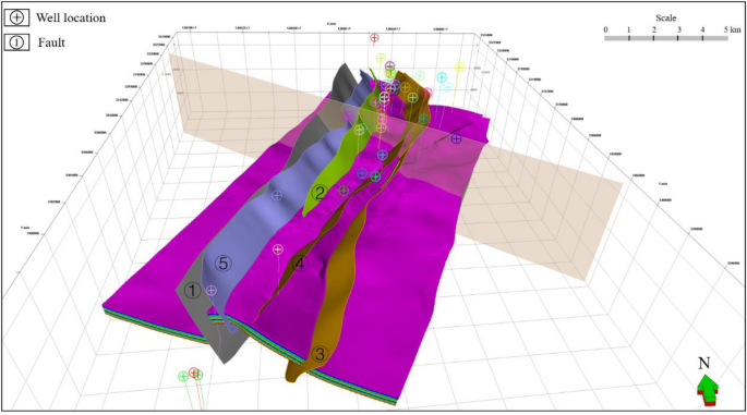
The 3D tectonic model of Xiangguosi UGS
Fig. 15 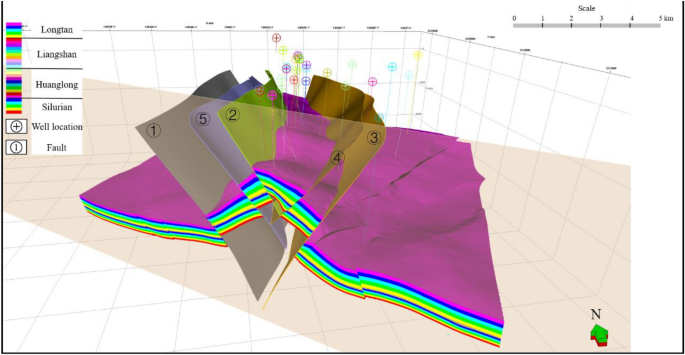
A fault profile of fault ①, fault ⑤, fault ②, fault ④, and fault ③
The normal pressure of five faults is all between 7.47 MPa and 51.24 MPa, higher than the ductility limit of 5 MPa, showing good fault-sealing properties (Table 5).
-
(iii)
The value of shear stress and normal stress could not be acquired directly. Referring to examples of geomechanical models used in Xiangguosi UGS from Zhao et al. [41], extracting parameters like intrinsic shear strength (cohesion) and internal friction coefficient, obtaining the relationship of shear stress and normal stress, then calculate the fault shear index.
Table 5 The table of basic data of normal pressure on the fault plane $$\frac{\tau }{\mu \times \text{(}\sigma -{\text{P}}_{\text{p}}\text{)}}\text{<}\frac{1}{{2}},$$(12)μ stands for the friction coefficient; Pp stands for the pore pressure, MPa.
μ is of 0.4–0.6, Pp is of 34–36 MPa [38].
$$\tau \text{<}\frac{1}{{2}} \times {0.4 \times (\sigma-36)}\text{ or }\tau \text{<}\frac{1}{{2}} \times {0.6 \times(\sigma -34)}\text{,}$$(13)$$\tau {<0.2 \sigma -7.2}\,\text{ or }\,\tau {<0.3 \sigma -10.2}.$$(14)$${I}_{c}=\frac{\tau }{C+\omega }.$$(15)$${{I}}_{{c}}<\frac{0.2 \sigma -7.2}{{0+0.4 \sigma}}{<0.5} \,{\text{or}}\, {{I}}_{\text{c}}<\frac{0.3 \sigma-10.2}{{0+0.6 \sigma}}{<0.5}.$$(16)Ic is always lower than 0.5 no matter how μ is taken. And there is no evident alternation in fault zones giving rise to good fault-sealing properties.
-
(iv)
Based on the 3D tectonic model of this study area, combining with the dip angle of both fault plane and reservoir stratum, extracting the imbrication depth of the cover and the depth of the cover, then calculate the vertical plugging coefficient (Table 6).
Table 6 The table of basic data of vertical plugging coefficient


The vertical plugging coefficient of five faults is all between 0.41 and 0.88, lower than 1, showing good fault-sealing properties.
For the comprehensive evaluation of fault-sealing in Xiangguosi UGS, see Table 7.
Although relevant parameters in mud shale can give way to those in gypsum salt rocks, information on Xiangguosi UGS is hard to obtain. Even if it’s acquired, the reliability is low. Therefore, assign the low value 2.5 to those that cannot be obtained, and put them into the calculation: IFS = 9 × 10% + 5 × 10% + 2.5 × 6% + 9 × 10% + 9 × 10% + 2.5 × 6% + 2.5 × 6% + 2.5 × 6% + 9 × 10% + 9 × 10% + 2.5 × 6% + 9 × 10% = 6.65, still higher than the median calculated in the example 5. It is believed that Xiangguosi is with good fault-sealing properties.
7.2 Application effect of Xiangguosi UGS
Xiangguosi UGS has been operating efficiently for 10 years, with a total of 158 × 108m3 gas injection and 128 × 108 m3 gas production. The workflow this paper concludes supports the design of construction key indicators and the first demonstration of “Expand the pressure range, increase the production” in China, which is the important basis point of the construction of the “signpost” UGS.
8 Conclusions
-
(i)
This paper summarizes the existing experience, systematically analyzes the adaptability of existing methods, and proposes an index to evaluate the fault-sealing capability of UGS. The methods start from three aspects of qualitative, quantitative, and mechanical stability evaluation based on the basic characteristics of faults, lithological configuration of the fault’s two blocks, analysis of production performance, Shale Smear Factor (SSF), Shale Gouge Ratio (SGR), properties of fault-filling materials, 3D tectonic model, normal pressure on the fault plane, fault shear index, and fault plugging coefficient, could provide a very complete and comprehensive evaluation of fault-sealing.
-
(ii)
Take the first UGS in SW China—Xiangguosi UGS as an example, selecting and improving parameters applicable to this study area, then develop the evaluation of fault-sealing. The calculation shows that five major faults are with excellent fault-sealing properties.
-
(iii)
The workflow this paper concludes supports the design of construction key indicators and the first demonstration of “Expand the pressure range, increase the production” in China, which is the important basis point of the construction of the “signpost” UGS, contributing to the efficient operation of Xiangguosi UGS for 10 years, with a total of 158 × 108 m3 gas injection and 128 × 108 m3 gas production.
Data availability
All data regarding the Xiangguosi UGS can be obtained from Chongqing Xiangguosi Underground Gas Storage Company Limited. However, restrictions apply to the availability of these data, which were used under license for the current study, and so are not publicly available.
References
Liang B, Wang W, Hao J. Evaluation on vertical sealing capacity of the main through faults, Malubei Area. Natural Gas Explor Dev. 2015;38(04):9–13.
Bian Q, Deng S, Lin H, Han J. Strike-slip salt tectonics in the Shuntuoguole Low Uplift, Tarim Basin, and the significance to petroleum exploration. Mar Pet Geol. 2022;139: 105600.
Bian Q, Wang Z, Zhou B, Ning F. Thin-skinned and thick-skinned tear faults in central Tarim Basin. J Asian Earth Sci. 2023;10: 100160.
Bian Q, Zhang J, Huang C. The middle and lower Cambrian salt tectonics in the central Tarim Basin, China: a case study based on strike-slip fault characterization. Energy Geosci. 2024;5(2): 100254.
Liu Z, Xin Q, Deng J. Formation mechanism and structural model of fault block group oil and gas reservoirs. Beijing: Petroleum Industry Press; 1998.
Lv Y, Fu G. Research on fault sealing. Beijing: Petroleum Industry Press; 2002.
Chai H. Sealing capacity of faults in tertiary Shahejie 3 Member, Qingxi area. Natural Gas Explor Dev. 2018;41(01):45–50.
Ma X, Zheng D, Shen R, Wang C, Luo J, Sun J. Key technologies and practice for gas field construction of complex geological conditions in China. Petrol Explor Dev. 2018;45(03):489–99. https://doi.org/10.11698/PED.2018.03.14.
Lindsay N, Murphy F, Walsh J, Watterson J, Flint S, Bryant I. Outcrop studies of shale smears on fault surface. Int Assoc Sedimentol Spec Publ. 1993;15:113–23. https://doi.org/10.1002/9781444303957.ch6.
Yielding G, Freeman B, Needham D. Quantitative fault seal prediction. AAPG Bull. 1997. https://doi.org/10.1306/522B498D-1727-11D7-8645000102C1865D.
Chen B. Subsurface geology. Petroleum Industry Press, 1987.
Wang K, Dai J. A quantitative relationship between the Crustal Streaa and fault sealing ability. Acta Petrol Sin. 2012;33(01):74–81. https://doi.org/10.7623/syxb201201009.
Fu X, Li K, Dong R, Li J. A review of research on fault sealing. Energy Technol Manage. 2021;46(03):24–6. https://doi.org/10.3969/j.issn.1672-9943.2021.03.010.
Peng P, Wu P, Peng H, Luo F, Wang Y, Shi X, Zhu Q. Calculating apparent stratigraphic dip under complex geological conditions and case study application to XC1 well. Natural Gas Explor Dev. 2019;42(03):127–32.
Liu Q, Li C, Lu L. Study on the fault sealing properties in Gaoyou Sag. J Oil Gas Technol. 2010;32(02):58–61. https://doi.org/10.3969/j.issn.1000-9752.2010.02.013.
Ma X, He X, Li J, Li Y, Chi Y, Chen Y, Liu C, Hao M. Study on fault sealing for Bannan underground gas storage. Mud Logging Eng. 2011;22(04):77–9. https://doi.org/10.3969/j.issn.1672-9803.2011.04.021.
Li C, Liu Q, Li Y, Chen J, Ye S, Zheng Y, Bi T. Research and application of fault sealing properties by the double-factor complementary method in Gaoyou Sag. Complex Hydrocarbon Reserv. 2012;5(02):1–4. https://doi.org/10.16181/j.cnki.fzyqc.2012.02.001.
Luo S, He S, Wang H. Review on fault internal structure and the influence on fault sealing ability. Adv Earth Sci. 2012;27(02):154–64. https://doi.org/10.11867/j.issn.1001-8166.2012.02.0154.
Tong H. Quantitative analysis of fault opening and sealing. Oil Gas Geol. 1998;03:45–50. https://doi.org/10.11743/ogg19980308.
Watts N. Theoretical aspects of cap-rock and fault seals for single- and two-phase hydrocarbon columns. Mar Pet Geol. 1987;4(4):274–307. https://doi.org/10.1306/948855de-1704-11d7-8645000102c1865d.
Allan U. Model for hydrocarbon migration and entrapment within faulted structures. AAPG Bull. 1989;73(7):803–11. https://doi.org/10.1306/94885962-1704-11D7-8645000102C1865D.
Zhao M, Li Y, Zhang Y, Wang D. Relation of cross-fault lithology juxtaposition and fault sealing. J China Univ Petrol (Edn Nat Sci). 2006;01:7–11. https://doi.org/10.3321/j.issn:1000-5870.2006.01.002.
Zhang H, Fang C, Gao X, Zhang Z, Jiang Y. Petroleum geology. Beijing: Petroleum Industry Press; 1999.
Ye Q, Wang M, Yang Z, Liang W, Gan Y. Comprehensive evaluation of fault lateral sealing ability in Wenchang A Area, Qionghai Swell, Pearl River Mouth Basin. Mar Origin Petrol Geol. 2018;23(04):81–6.
Chen S. Research on the structural evolution and fault sealing of Fuyu reservoir in Chaoyang Area. Songliao Basin: China University of Geosciences (Beijing); 2009.
Cao L, Wang S, Gao P, Zhang L, Yue H. Fault sealing of neogene lithology–structural reservoirs in the Huanghekou Sag. Fault-Block Oil Gas Field. 2022;29(04):502–7.
Zhang D. Study on UGS sealing evaluation of fault-block oil & gas reservoir—a case study of the Banzhongbei UGS in Dagang Oilfield. J Guangdong Univ Petrochem Technol. 2018;28(03):30–3.
Zhang X. Sealing mechanism and closure evaluation methods of carbonate fault. Liaoning Chem Indus. 2018;47(02):110–2. https://doi.org/10.14029/j.cnki.issn1004-0935.2018.02.008.
Wang S, Han F, Sun Z, Bing Q, Wang L, Xu B. Present situation and the development trend of in-situ stress measurement and its effect on hydrocarbon migration and fault block. Prog Geophys. 2021;36(02):675–88. https://doi.org/10.6038/pg2021EE0212.
Zha M, Wu K, Qu J, Chen Z. Migration pathway and entrapment of hydrocarbons in faulted basins. China: China University of Petroleum Press; 2008.
Shi B, Guan D, Zhou K. Yangtze marine geology and oil & gas. Beijing: Petroleum Industry Press; 1993. p. 262–9.
Fu G, Yin Q, Du Y. A method studying vertical seal of fault with different filling forms and its application. Petrol Geol Oilfield Dev Daqing. 2008;125(01):1–5. https://doi.org/10.3969/j.issn.1000-3754.2008.01.001.
Zhu C, Wang W, Wang Q, Li Y. Numerical simulation of structural strain for turbidite sands reservoirs of low permeability. J Jilin Univ (Earth Sci Edn). 2016;46(05):1580–8. https://doi.org/10.13278/j.cnki.jjuese.201605306.
Li H, Wu J, Huang J, Wang Y, Li Z. Quantitative analysis of fault vertical sealing ability and its application in a oilfield of Bohai Bay Basi. Bull Geol Sci Technol. 2020;39(04):125–31. https://doi.org/10.19509/j.cnki.dzkq.2020.0416.
Tan L, Xie H, Zhang H, Zhao J, Guo Y. A quantitative research method on the sealing of growth faults: a case study of JX1-1 oil field in Liaozhong Sag, Liaohe depression. Petrol Geol Exp. 2018;40(02):268–73. https://doi.org/10.11781/sysydz201802268.
Yin H, Lang N, Zhou X, Cao S, Wang P, Xu G. Comprehensive evaluation of fault hydraulic conductivity based on fault sealing and numerical simulation. Saf Coal Mines. 2022;53(03):200–7.
Fu X, Lv Y, Fu G, Wen H. Quantitative simulation experiment and evaluation method for vertical seal of overthrust. Chin J Geol. 2004;02:223–33. https://doi.org/10.3321/j.issn:0563-5020.2004.02.009.
Wang L, Xu H. Advances of research on fault sealing. J Xinjiang Petrol Inst. 2003;01:11–5. https://doi.org/10.3969/j.issn.1673-2677.2003.01.003.
Liu Y, Yu X, Li S. On the comprehensive evaluation of fault sealing of ken east fracture zone using fuzzy method. J Chongqing Univ Sci Technol (Nat Sci Edn). 2009;11(02):11–3. https://doi.org/10.19406/j.cnki.cqkjxyxbzkb.2009.02.004.
Shen C, Mei L, Tang J, Du X. New advances of researches on fault sealing. Fault-Block Oil Gas Field. 2002;04:1–5. https://doi.org/10.3969/j.issn.1005-8907.2002.04.001.
Zhao Y, Luo Y, Li L, Zhou Y, Li L, Wang X. In-situ stress simulation and integrity evaluation of underground gas storage: a case study of the Xiangguosi underground gas storage, Sichuan, SW China. J Geomech. 2022;28(04):523–36. https://doi.org/10.12090/j.issn.1006-6616.2021138.
Acknowledgements
Chongqing Xiangguosi Underground Gas Storage Company Limited is thanked for access to data. We thank the reviewers for comments.
Funding
This study is supported by Research and Field Tests on Key Technologies for Efficient Reservoir Construction of Carbonate Rock Gas Reservoir (2022KT2303), Major Science and Technology Project of China National Petroleum Corporation.
Author information
Authors and Affiliations
Contributions
Ruoyu Mu and Yu Luo wrote the main manuscript text. Zihan Zhao and Yuan Zhou built the framework for the initial article and took on the management work. Yuchao Zhao helped draw figures. Mengyu Wang helped translate the manuscript. Limin Li provided relevant data of Xiangguosi Underground Gas Storage. All authors reviewed the manuscript.
Corresponding author
Ethics declarations
Conflict of Interest
The authors have no relevant financial or non-financial interests to disclose.
Additional information
Publisher's Note
Springer Nature remains neutral with regard to jurisdictional claims in published maps and institutional affiliations.
Rights and permissions
Open Access This article is licensed under a Creative Commons Attribution 4.0 International License, which permits use, sharing, adaptation, distribution and reproduction in any medium or format, as long as you give appropriate credit to the original author(s) and the source, provide a link to the Creative Commons licence, and indicate if changes were made. The images or other third party material in this article are included in the article's Creative Commons licence, unless indicated otherwise in a credit line to the material. If material is not included in the article's Creative Commons licence and your intended use is not permitted by statutory regulation or exceeds the permitted use, you will need to obtain permission directly from the copyright holder. To view a copy of this licence, visit http://creativecommons.org/licenses/by/4.0/.
About this article

Cite this article
Mu, R., Luo, Y., Zhao, Z. et al. Evaluation of fault-sealing: a case study on Xiangguosi underground gas storage, SW China. Discov Appl Sci 6, 270 (2024). https://doi.org/10.1007/s42452-024-05933-y
Received:
Accepted:
Published:
DOI: https://doi.org/10.1007/s42452-024-05933-y