
Abstract
Rain attenuation becomes the prime reason for link failure at frequencies above 10 GHz. C band and Ku band are already exhausted for Indian region satellite communication and time has come to shift to next higher Ka-band. But the attenuation due to rain is very large for this band, especially for tropical country like India. This has led to the development of many rain attenuation prediction models. But to apply rainfall data in these models, fine rainfall data is required which is not available for most locations, and if available, are not for longer durations. In this paper, a novel method is described that can be used for rainfall attenuation prediction for India using coarse rainfall data, that is available from Indian Meteorological Department. Many models are available to predict the 1 min integration rainfall distribution around the world. But for Indian subcontinent, most models show large variations from actual rainfall attenuation. This paper presents estimation of rainfall attenuation for Ka-band for five different regions covering almost whole India using ITU-R model, Crane-Global model and Moupfouma model. These estimations are compared with actual measured results of previous works. The calculated rainfall rates suggest significant variances in the mean rainfall intensity or rate in mm/h. The analysis shows that the ITU-R model overestimates the rainfall intensity rates when empirical model is developed using data from Indian Meteorological Department. It is observed that ITU-R model is best suited for Indian region, but needs modifications to obtain accurate estimation for rain attenuation. Hence a new empirical model named Dafda–Maradia model for rain attenuation for India is proposed. This model is based on ITU-R model and is basically a modified ITU-R model. Here the prediction of rainfall attenuation is done from coarse rain data of 64 years (1951–2014). It is observed that there is a large decrease in the average rainfall intensity as compared to the ITU-R model.
1 Introduction
Rain attenuation is the major cause of link failure in Ka-band, as other attenuation is only few dBs. For heavy rainfall the signal becomes very similar to the noise signal of the receiver and hence is inseparable. But Ka-band is more attractive due to wide bandwidth available. Ka-band is under experimentation stage and will soon be utilized for future satellite communication in India. GSAT-14, the 23rd Geostationary Satellite launched by ISRO-India in January, 2014 has two Ka band Beacons operating at 20.2 GHz and 30.5 GHz to carry out attenuation studies as their two payloads [1]. Indian Meteorological Department keeps a record of monthly rainfall for 36 meteorological subdivisions since many years [2]. For precise calculations of rainfall attenuation the rain data collected should be as long as possible. Keeping in mind this fact the rain attenuation prediction is done from 64 years (1951–2014) data for India. The predictions are made at the downlink frequency of Ka-band (20.2 GHz), for the monsoon months of India. i.e. June, July, August and September (JJAS). Predictions using ITU-R model, Crane Global model and Moupfouma model are done and modified ITU-R model namely Dafda–Maradia model is proposed for India. The rainfall attenuation values suggested by Dafda–Maradia model are matching closely with the values obtained from previous works and prove the accuracy of the model for Indian region. Similar modifications in ITU-R model are suggested for Ku-band for tropical stations in [3,4,5]. Hence a modification in ITU-R model for Ka-band is desirable and necessary for India.
2 Rainfall intensity calculations
Climatic impacts like rain attenuation, cloud constriction and so on are frequently indicated on a percent of time premise [6, 7]. The Rainfall rate/force is normally determined for a particular blackout rate. This rate is typically 0.01% of a normal year. The blackout rate is characterized as a factual computation that is utilized to anticipate the level of time that rain attenuation surpasses a specific limit. On the off chance that level of surpassed time is 100%, it implies it rains intensely each of the 365 days or 8760 h and connection is fizzled for every one of the 8760 h. Correspondingly, in the event that it is 1%, it implies downpour surpasses for 87.60 h in a year causing link failure, in the event that it is 0.01%, it implies link fails for 0.876 h or 52.56 min in a year. Practically all models are determined for 0.01% rainfall exceedance. A wide range of terms are utilized for indicating the percent of time variable. This incorporates outage percentage, blackout rate, exceedance rate, accessibility, reliability or dependability. On the off chance that the time parameter is the percent of time surpassed, P, at that point (\(100-\) P) speaks to the connection accessibility or link reliability.
Hence an exceedance probability of 0.01% means an expected outage of 0.01% or 53 min per year and it denotes a link availability of 99.99%. For rainfall estimation we consider exceedance probability rather than the non-exceedance probability. Exceedance probability (p) gives the probability that certain rainfall or higher will occur in a given year. The equation for exceedance probability is same except the fact that rank m receives value 1 for highest value of rainfall.
Here n is number of data points (number of years in this case). This is a very useful statistic for heavy rainfall prediction, where we are interested in the probability of a certain amount of rainfall or more that might cause link failure.
To predict the rainfall rate at a particular location, appropriate rainfall distribution at the site must be available. Also the rainfall distribution must be obtained from long term measurement data with 1 min integration time. Longer integration time rainfall rate is not used as it fails to capture high intensity short duration rainfall and so it is not recommended for communication system design. Therefore for attenuation prediction studies, 1 min integration time is accepted worldwide as most appropriate. The rainfall data available from IMD website is yearly and monthly and we need to have 60 min integration rainfall data to be applied to Rain rate Statistics conversion MATLAB program provided by ITU-R P837.7 [8]. This program gives us the 1 min integration rain rate, which can be applied to ITU-R model for attenuation predictions.
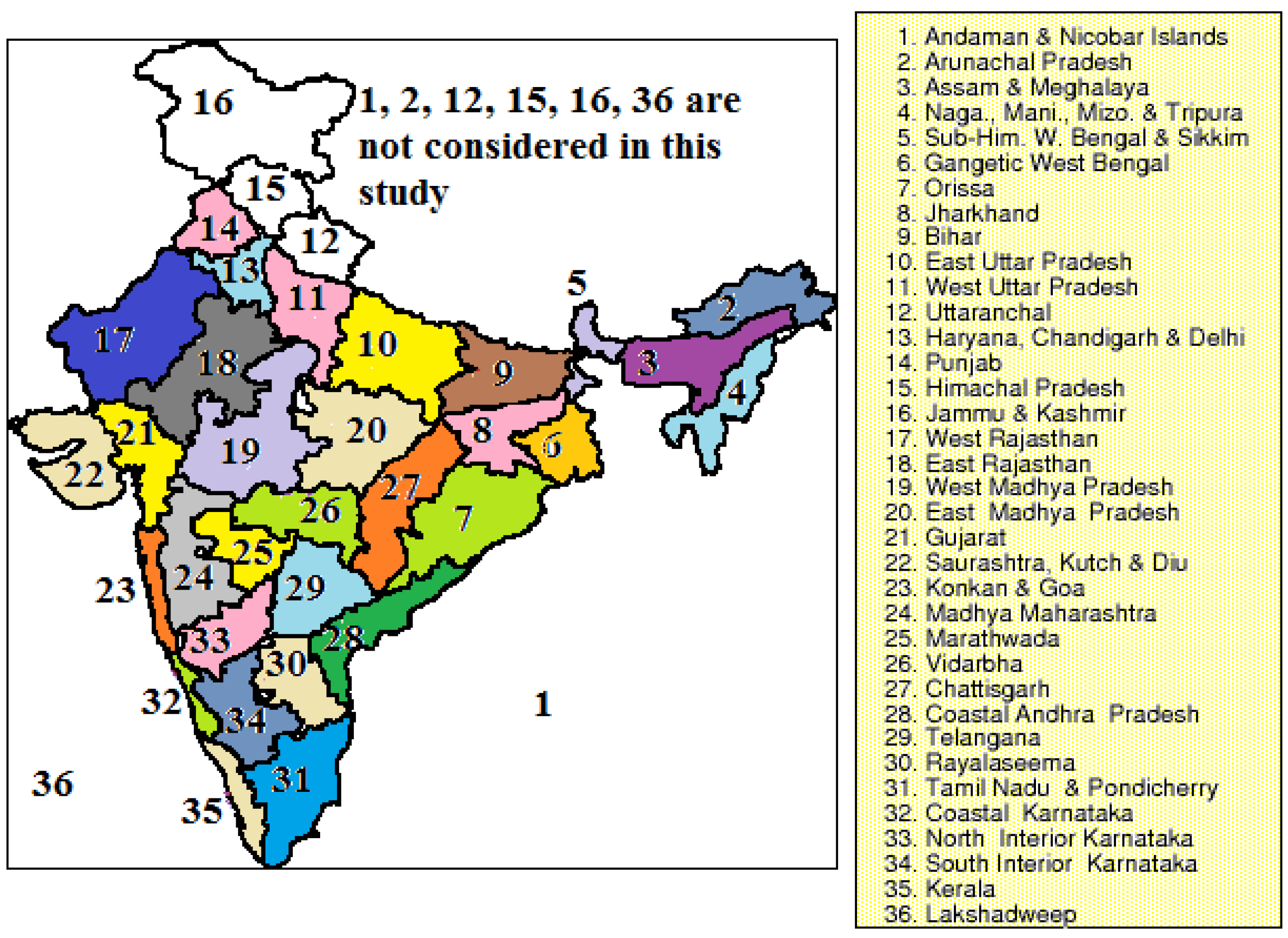
Indian Meteorological Department keeps the record of rainfall data of 36 meteorological-subdivisions [2]. This data is monthly, seasonal as well as annual rainfall data in mm. These 36 meteorological subdivisions are shown in Fig. 1 below.

36 Meteorological subdivisions of India [9]
The 36 Meteorological subdivisions of India can be grouped under different regions of India as per Table 1 below.
For present work 5 different subdivisions’ data is chosen to cover 5 different regions of India as mentioned in Table 2 below.
The regions were so chosen that almost every region of India is covered and overall model can be suggested for whole India. A unique method was developed for rainfall intensity and hence rainfall attenuation calculation which uses the coarse rainfall data instead of traditional method of using fine rainfall data. The obvious advantage is that the estimation can be done for a very long duration (64 years in the present work). For example say the fine rainfall data is available for 3 years and rainfall exceedance calculations are made. But it may happen that the rainfall was below average for those 3 years. Hence overall results may be misguiding. Conclusively and statistically as long as the data is used, the more precise the calculations can be made.
The step by step method employed for estimation of rainfall attenuation using coarse rainfall data is as follows:
-
1.
The monthly rainfall data is collected from IMD website [10]. This rainfall is in mm.
-
2.
The rainfall data of particular month is arranged in descending order, giving the highest rainfall rank 1. For monsoon in India, June, July, August and September (JJAS months) are chosen. Hence 122 days long monsoon period is chosen.
-
3.
Monthly data is converted to daily data by simple averaging method.
-
4.
Next, the exceedance probability for all ranks is calculated using, \(\hbox {p} = \hbox {m}/(\hbox {n}+1)\), where m is the rank value and n is number of data points (number of years (64) in this case).
-
5.
Find out return period using formula \(\hbox {T} = 1/\hbox {p} = (\hbox {n}+1)/\hbox {m}\), where again m is the rank and n is data points and p is exceedance probability.
To find out rainfall intensity in mm/h, we have used the IDF(Intensity, Duration, Frequency) equations for Indian region developed by Kothyari and Garde [11]. Intensity–Duration–Frequency (IDF) curves describe the relationship between rainfall intensity, rainfall duration, and return period (or its inverse, probability of exceedance). IDF curves are commonly used in the design of hydrologic, hydraulic, and water resource systems [12]. Kothyari and Garde developed an equation for the rainfall intensity, duration and frequency with the Indian conditions. They developed the equation for IDF curves using the rainfall data of 78 rain gauge stations from all over India considering the value of mean annual rainfall (R) for 24 h, and 2-year rainfall, \(R_{24}^{2}\) [13].
Intensity Duration Frequency (IDF) is a measurable connection between the rain intensity (I), the duration (D), and the return time period (T), [14]. First the month to month information is changed over to every day information by straightforward averaging technique. At that point utilizing Kothyari and Garde equation, the rain intensity for specific month of a specific year is discovered. This equation is [14],
where, \(I_{t}^{T}\) is the precipitation force (rain intensity) in mm/h
-
T return period in years and t span of rain in h
-
\(R_{24}^{2}\) is 24 h, a 2-year return period precipitation in mm
-
t t is picked be 1 h as we need a hour incorporation precipitation information to be connected to Rain rate measurements change MATLAB program [8] that changes over a hour reconciliation precipitation to 1 min coordination precipitation.
Here estimations of steady C in various geographical regions of India proposed by them [11] are given in the Table 3. For instance as Ahmedabad is in western India, the estimation of C can be taken as 8.3 and for New Delhi (northern India) C is picked as 8.0. Likewise for Bhopal, C is 7.7, for Kolkata C is 9.1 and for Bengaluru C is 7.1.
-
6.
Now we have obtained the rainfall intensity in mm/h for particular month of a particular year. This rainfall intensity is 60 min or 1 h integration rainfall. But to provide the values to ITU-R model, we need to have 1 min integration rainfall rate. This is done by using Rain rate Statistics conversion MATLAB program provided by ITU-R P837.7 [8]. The inputs required to be given to the software are:
-
(a)
T-minute integrated P(R): percentage exceedance value between (0–100%)
-
Normally three values are provided with spaces in between: 0.01 0.1 1
-
-
(b)
T-minute integrated P(R): rain rate values (mm/h)
-
Corresponding rain rate values for 0.01%, 0.1% and 1% should be provided
-
-
(c)
Source integration time (minutes)
-
As we are providing values for 60 min, 60 is the input
-
-
(d)
Station details (latitude and longitude).
-
(a)
The GUI of ITU-R P837-7 in which inputs for Bengaluru city is shown in Fig. 2 below.

ITU-R P.837-7 rain rate statistics GUI with inputs given for Bengaluru City
After providing inputs, the conversion is run in MATLAB [15]. The output of the software is a figure depicting both the T-minute integrated input P(R) with blue line and the 1 min integrated output P(R) with red line. Figure generated for JJAS months of Bengaluru is shown in Fig. 3.

The software also generates data files P1.dat and R1.dat that generates respectively the probability and rain rate vectors of the estimated 1 min integrated P(R), and data file Log_PL_coeffs.dat that contains the values of power law expression defining the estimated 1 min integrated P(R). Figure 3 shows that for 0.01% exceedance probability, the 60 min measured Rain rate (mm/h) provided to the GUI is 36.55 mm/h and the corresponding 1 min estimated rain rate is 101.45 mm/h. This GUI software is very useful since it gives the corresponding 1 min integrated rainfall rate from 60 min measured values. Always 1 min integrated rain rate values are required to be provided to different models for correct rain attenuation estimations. The importance of 1 min integration rain rate values is that some rainfall may be of very small durations but of very high intensities.
-
7.
The data files P1.dat and R1.dat are provided to ITU-R model [16] for calculation of rainfall attenuation. Also same data files can be applied to other models for finding Rain attenuation.
Calculations were initially carried out for monsoon months JJAS (June, July, August and September) of New Delhi and Ahmedabad and later the work was extended to cover other cities namely Bhopal, Kolkata and Bengaluru. Hence cities were chosen to cover all regions of India like New Delhi (Northern India), Ahmedabad (Western India), Bhopal (Central India), Kolkata (Eastern India) and Bengaluru(Southern India). Chennai was not chosen from south India since it receives its maximum rainfall through northeast monsoon during the months of October to December [17], whereas primary rain season of Bengaluru is June to September [18]. We have provided the following parameters in different models for the calculation of Rain Attenuation(RA) at 20.2 GHz Ka-band downlink frequency for different cities of India (Table 4).
The parameters for all cities have been taken from Satellite Earth Stations of respective cities[19,20,21,22,23].The data files P1.dat and R1.dat are provided to ITU-R model [16] for Calculation of Rain attenuation. Also same 1 min integrated rain rate R1.dat is applied to Crane-Global model [7] and Moupfouma model [24] to calculate the rain attenuation. This technique is encouraged to be utilized in all pieces of the world which expressed that the rain attenuation should be considered for any working frequencies past 5 GHz and for frequencies up to 100 GHz with way lengths up to 60 km [25]. The first Global Crane model is taken for our examination for Indian locale. A correction of this Crane model is known as the two-component model that represents both the thick focus and periphery territory of a rain cell [26]. The modified ITU model is the DAH model (1997) [27]. According to Garcia [28], the database used to derive the prediction method is an extension of the ITU-R database of rain attenuation in terrestrial links, to which results of measurements carried out in the South-eastern region of Brazil have been added. Hence for Indian region, the applicable models can be ITU-R model[16], Crane-Global model[7] and Moupfouma model[24] and so these are applied for our study of rain attenuation. These three models (ITU-R, Crane and Moupfouma) are applied for rain attenuation calculation and the results are obtained which are discussed below.
3 Results and discussion
The 0.01% rainfall intensity for 1 min integration time using method described above was applied to ITU-R model and it was found that the rainfall intensity values found was varying largely as compared to the values suggested by ITU-R P-837-7 [8]. Hence a new modified ITU-R model is suggested for India and is named as Dafda–Maradia model. The mean rainfall intensity values suggested by ITU-R model is shown in Fig. 4.

Based on the method described using Kothyari and Garde equation [11], rainfall intensity was calculated for 5 different regions of India—North India, West India, Central India, East India and South India. Finally Rain attenuation model namely Dafda–Maradia model shown in Fig. 5 is proposed for India. This model is a modified ITU-R model, which is having different rain intensity values for different regions of India as compared to values suggested by ITU-R [8, 29].

Rain attenuation Dafda–Maradia model for India
The rainfall intensity values suggested by ITU-R P 837-7 [8, 29], for different regions of India are shown in Table 5. Also estimated rain intensity values using DM (Dafda–Maradia) model are shown next to it. The difference between ITU-R and DM model is shown in the next column.
From the table it is visible that Dafda–Maradia model shows a variation from 20 to 50% as compared to values given by ITU-R [8]. The values are much less as compared to ITU-R model. While designing the fade mitigation systems, these values suggest a large saving of power and cost.
The 0.01%, 1 min integration Rain Rate values obtained from ITU-R P837.7 [8], are also applied to Crane-Global model and Moupfouma model and the mean attenuation values obtained for all models are compared in Table 6.
ITU-R model rain attenuation values are calculated from ITU-R model rain rate values [8, 29]. Dafda–Maradia (DM) rain attenuation values are calculated using rain rate values suggested by DM model (Table 5).
Following comparisons from previous works done for Ka band proves that Dafda–Maradia model is more accurate for India as compared to other models:
-
(1)
For New-Delhi, applying ITU-R model, 25 dB is predicted in [30]. This proves that the rain rate value suggested for New-Delhi in ITU-R model is more as compared to actual average rain rate value. Also, actual measured value using frequency beacons of GSAT-14 is 22 dB. Our Dafda–Maradia model gives value of 23.12 dB. Hence% error with ITU-R model is (\(25-22 = 3\hbox { dB} = 12\,\%\)) and % error with Dafda–Maradia model is (\(23.12-22 = 1.12\hbox { dB} = 4.85\%\)). This proves that Dafda–Maradia model is much accurate as compared to ITU-R. For same New-Delhi, Crane-Global and Moupfouma model much underestimates the rain attenuation.
-
(2)
For Umiam, Meghalaya [31] the beacon attenuation measured for GSAT-14 gives an attenuation of 21 dB for rain rate of 42 mm/h, which is matching with attenuation of Ahmedabad (41.56 mm/h\(- 25.22\) dB) obtained using Dafda–Maradia model. For Umaim latitude is \(25.67^{\circ }\hbox { N}\) and for Ahmedabad latitude is \(23.03^{\circ }\hbox { N}\). If parameters of Ahmedabad are replaced by parameters of Umiam in the same program, for Rain rate of 42 mm/h, Rain attenuation obtained is 20.82 dB 21 dB (the same value that is obtained using beacon measurement at Umiam). This again proves the authentication of Dafda–Maradia model for India.
-
(3)
In the paper [32], for RR of 40 mm/h in Singapore, rain attenuation measured using beacons is 20 dB, for 99.99% link availability. As Singapore is a tropical country, conditions are identical to India.
The ITU-R model is applied and modified since it is widely accepted, continuously updated and used by many researchers worldwide [16, 30, 33]. Moupfouma model much underestimates the rain attenuation for India, whereas Crane-Global model shows large variations in predictions as can be seen from Table 6 above. The predicted rain attenuation exceeded for 0.01% of an average year for ITU-R P 618 [16] is given by:
where \(A_{0.01}(\hbox {ITU-R}) = 0.01\,\%\) rain attenuation value obtained using ITU-R model in dBs \(\gamma _R =\) Rain specific attenuation \(L_E =\) effective path length While the predicted rain attenuation value for 0.01% of an average year for DM (Dafda–Maradia) model is given by:
where \(A_{0.01}(\hbox {DM}) = 0.01\,\%\) rain attenuation value obtained using Dafda–Maradia model in dBs \(A_{0.01}(\hbox {ITU-R}) = 0.01\,\%\) rain attenuation value obtained using ITU-R model in dBs \(D =\) Constant in dB having value as given in Table 7 below.
Consider for example, for New-Delhi ITU-R model suggests RA of 31.85 dB. So, to find out RA due to Dafda–Maradia model, as per DM equation above,
\(A_{0.01}(\hbox {DM}) = A_{0.01}(\hbox {ITU-R}) - D\hbox { dB} = 31.85 - 8.7\hbox { dB}\) ( As, New-Delhi is in North India, constant \(D = 8.7\) as per Table 7 above) \(= 23.15\hbox { dB}\).
The obtained value 23.15 is matching with DM model dB value (23.12) as shown in Table 6 above. Similarly for Ahmedabad value is, 28.6 – 3.4 (West India) \(= 25.2\hbox { dB}\) 25.22 as per Table 6.
Applying mean values of rain rate and finding out rain attenuation for other percentages of time, gives cumulative distribution of rain attenuation for different cities (zones) of India. Figure 6 shows the cumulative distribution of rain attenuation for New-Delhi.

Cumulative distribution of rain attenuation for New-Delhi (North-India)
As can be seen from Fig. 6, ITU-R model much overestimated the Rain Rate and hence Rain attenuation for New-Delhi. Here for 0.01% rain exceedance (99.99% link availability), ITU-R model gives attenuation of 31.85 dB, whereas for same availability, Dafda–Maradia model gives attenuation of 23.12 dB. Crane model gives attenuation of 19.41 dB and Moupfouma gives attenuation of 16.2 dB for the same availability. The value of rain attenuation drops down to 8.99 dB for 0.1% exceedance value using Dafda–Maradia model. This value is very useful and manageable rain attenuation value for 99.9% link availability. Fade mitigation techniques can be designed accordingly. If only 99% link availability is required, RA is only 2.17 dB using DM model.

Cumulative distribution of rain attenuation for Ahmedabad (West-India)
Figure 7 shows the cumulative distribution of RA for Ahmedabad and hence west India. DM model shows an average value of 25.22 dB for 0.01% rain exceedance, whereas ITU-R model, Crane model and Moupfouma model gives a value of 28.6 dB, 22.53 dB and 18.5 dB respectively. Crane model and Moupfouma underestimates the RA for Ahmedabad while ITU-R overestimates the RA for Ahmedabad. For 0.1% and 1% rain exceedance the rain attenuation lowers to 10.47 and 2.41 respectively using DM model. Hence it is feasible to operate link at these rain exceedance.
As can be seen from Fig. 8, the calculated cumulative statistics of rain attenuation is over – estimated by ITU-R model for Bhopal (Central India). The over estimation becomes highly pronounced at lower time percentage. For instance, the calculated RA values using DM model are 10.60 dB, 25.58 dB and 42.91 dB respectively at 0.1%, 0.01% and 0.001% of the time while ITU-R predicts 13.85 dB, 32.59 dB and 53.32 dB respectively. An opposite pattern is observed with the application of Crane Global model and Moupfouma models which underestimates the measured rain attenuation values, particularly at 0.001% and 0.01% of the time.

Cumulative distribution of rain attenuation for Bhopal (Central-India)
It is interesting to note that Crane model almost matches the values given by DM model for Kolkata in Fig. 9. The reason is that Kolkata comes in H region of Crane model map[7]. This means that Crane model is matching DM model for East India. Hence Crane model is well applicable towards eastern part of India. But RR values suggested by ITU-R model are still much higher for East India and hence ITU-R model overestimates the values of RA for Kolkata. For 0.01% of time, ITU-R model gives RA value of 40.9 dB, Moupfouma model gives RA of 20.98 dB, Crane model gives RA value of 27.48 dB and DM gives RA value of 26.74 dB. Even for 0.1% rain exceedance, ITU-R suggests RA value of 17.88 dB while DM suggests RA value of 11.19 dB. Hence link failure will occur even for 0.1% of time as per ITU-R model, but link operation is possible as per DM model by proper amplification of signal.

Cumulative distribution of rain attenuation for Kolkata (East-India)
As can be seen from Fig. 10, ITU-R model much overestimates the RR and hence RA for south India, while Crane model and Moupfouma model much underestimates the RA for south India. Interestingly these models give closer estimation of RA for higher time percentages P > 1%. For 0.01% of time ITU-R model, DM model, Crane model and Moupfouma model gives estimated RA of 38.48 dB, 23.46 dB, 16.57 dB and 15.48 dB respectively. Even for 0.1% of time, that is 99.9% link availability, ITU-R model estimates high attenuation of 18.61 dB whereas DM model estimates RA of 10.78 dB. Hence from Figs. 6, 7, 8, 9 and 10, it is concluded that Moupfouma and Crane model much underestimates the RA for most part of India, while ITU-R model much overestimates the RA for whole of India. This is due to the predicted average RR values for 0.01% of time, which are much higher given by ITU-R model [5, 33]. While the RR values calculated by DM model are much lower than ITU-R model. The RA values for 0.01% of time (99.99% link availability) ranges from 23 to 27 dB as per DM model proposed for India. Keeping in mind rain variability for different regions of India, it can be concluded that average RA for 0.01% of time varies from 20 dB to 30 dB for any location in India.

Cumulative distribution of rain attenuation for Bengaluru (South-India)
Figure 11 shows overall 0.01% RA for JJAS months for different cities (regions) of India using DM model. This figure also shows the maximum value of rain that has occurred in a particular city in last 64 years (1951–2014). As can be seen from Fig. 11 for very rare heavy rainfall of 110.20 mm/h, RA can reach up to 40.92 dBs. But its probability of occurrence is lowest and return period is highest. The highest rainfall for Ahmedabad (West India) can reach up to 109.55 mm/h for which RA reaches up to 44.75 dBs. Hence for almost same value of maximum rainfall, attenuation for Ahmedabad is around 5 dBs higher as compared to New-Delhi. This is due to location of Ahmedabad towards western part of India. The maximum RR for Bhopal (Central India) reaches to 120.13 mm/h for which RA occurring is 46.15 dB. The RA occurring for Bhopal will be lower as compared to Ahmedabad while higher as compared to Kolkata due to its Central India location. The RR occurring for Kolkata (East India) is highest (133.56 mm/h) as compared to all other parts of India, but RA (47.34 dBs) occurring is higher than New-Delhi (North India) and lower than other parts of India as can be observed from Fig. 11. For Bengaluru (South India) maximum rain intensity that occurs is 117.80 mm/h for which rainfall attenuation is 51.57 dBs. Also it can be observed for Fig. 11 above that maximum RA in India occurs for South India. Hence it can be concluded that maximum RA occurs for Bengaluru (South India); then comes Ahmedabad (West India), Bhopal (Central India), Kolkata (East India) and New-Delhi (North India) in the decreasing order. Rainfall Intensity is independent of the location and is more usually for Eastern (Kolkata) and Central (Bhopal) India. These values are overall total attenuation and mean/average values of attenuation are important which are given in Table 6 above.

Comparison of rain attenuation for different cities (regions) of India using DM model
Table 8 shows Rain intensity values (0.01%) for five different regions of India obtained using Dafda–Maradia model and corresponding mean attenuation values for these five regions. Also standard deviation above and below mean attenuation values is shown. This gives the range of probable rain attenuation for these regions of India. As can be seen from Table 8, maximum average RA occurs for East India while minimum average RA occurs for North India.
Finally Table 9 shows the 0.01% rainfall intensity/rate values suggested by ITU-R P 837-7 [8, 29] for different cities of India and corresponding Rain Attenuation(RA) values found using ITU-R model and DM model which is helpful in applying different fade mitigation techniques for these cities.
As can be seen from cities mentioned in Table 9, RA is maximum for Madurai city (52.86 dB) as per ITU-R model but as per DM model RA is maximum for Mumbai city (42.66 dB) for 0.01% of time which is actually true as per rain history of India. Minimum rainfall occurs in Srinagar as per ITU-R model (13.09 dB) as well as DM model (4.39 dB). The variation of Rainfall is around 35 dB as per ITU-R model, while it is around 25 dB as per DM model.
4 Conclusion
The 0.01% Rain Rate values suggested by ITU-R model are much larger as compared to actual Rain Rate values calculated from the Monsoon Rainfall data (JJAS months-June, July, August and September months) of 64 years obtained from IMD. Due to predictions from longer duration of data, statistical accuracy is obtained. Consequently a new Rain attenuation model namely Dafda–Maradia model is proposed for India. The DM model suggests a reduced Rain Attenuation as compared to that suggested by ITU-R model. The rain attenuation proposed is 5–15 dB lower than as defined by ITU-R model. DM model is proposed taking data from 5 meteorological subdivisions. If still more meteorological subdivisions are taken in account, more accuracy can be obtained using Dafda–Maradia model and hence larger saving of power can be achieved while applying fade mitigation techniques.
References
GSAT-14-ISRO, https://www.isro.gov.in/Spacecraft/gsat-14-0
Area Weighted Monthly, Seasonal And Annual Rainfall (in mm) For 36 Meteorological Subdivisions—Open Government Data (OGD) Platform India. https://data.gov.in/resources/area-weighted-monthly-seasonal-and-annual-rainfall-mm-36-meteorological-subdivisions
Yussuff AI, Khamis NH (2013) Modified ITU-R rain attenuation prediction model for a tropical station. J Ind Intell Inf 1:155–159
Yaccop AH, Yao YD, Ismail AF, Badron K, Hasan MK (July-2016) Refining Ku-Band Rain Attenuation Prediction using Local Parameters in Tropics, Indian Journal of Science and Technology. J Ind Intell Inf 9(25)
Kestwal MC, Joshi S, Garia LS (April 2014) Prediction of Rain Attenuation and Impact of Rain in Wave Propagation at Microwave Frequency for Tropical Region (Uttarakhand, India). Int J Microw Sci Technol
Dissanayake A, Allnutt J, Haidara F (1997) A prediction model that combines rain attenuation and other propagation impairments along Earth-satellite paths. IEEE Trans Antennas Propag (USA) 45(10):1546–1558
Crane RK (1980) Prediction of attenuation by rain. IEEE Trans Commun COM–28(9):1717–1733
ITU-R P.837-7, Characteristics of precipitation for propagation modelling (2017)
Meteorological Subdivisions—Open Government Data (OGD) Platform India. http://www.mdpi.com/climate/climate-03-00858/article_deploy/html/images/climate-03-00858-g001.png
Rainfall in India—Open Government Data (OGD) Platform India. https://data.gov.in/catalog/rainfall-india
Kothyari UC, Garde RJ (1992) Rainfall intensity-duration-frequency formula for India. J Hydraul Eng ASCE 118:323–336. https://doi.org/10.1061/(ASCE)0733-9429(1992)118:2(323)
IDF Procedure, Retrieved from http://www.engr.colostate.edu/~ramirez/ce_old/classes/cive322-Ramirez/IDF-Procedure.pdf
Zope PE, Eldho TI, Jothiprakash V (2016) Development of rainfall intensity duration frequency curves for Mumbai City, India 2016. J Water Resour Prot 8:756–765. https://doi.org/10.4236/jwarp.2016.87061
Koutsoyiannis D, Demosthenes K, Manetas A (1998) A mathematical framework for studying the rainfall intensity-duration-frequency relationships. J Hydrol 303:215–230
www.mathworks.com, The Mathworks, Inc. Protected by U.S. and International Patents
ITU-R P 618-7, Propagation data and prediction methods required for the design of Earth-space telecommunication systems (2001)
NORTHEAST MONSOON. http://www.imdchennai.gov.in/northeast_monsoon.htm
Bangalore facts—Temperature—Rainfall. https://www.karnataka.com/bangalore/facts/
ISRO, MOSDAC-Meteorological and Oceanographic Satellite Data Archival Centre, Space Applications Centre, ISRO, 2017. www.mosdac.gov.in
DishPointer, DishPointer, Satellite Finder/Dish Alignment Calculator with Google Maps, 2017. www.dishpointer.com
Jeena J (July-2012) A study of rain attenuation calculation and stretegic power control for Ka-band satellite communication in India, M.Tech-Thesis, National Institute of Technology, Rourkela
Maitra A, Chakravarty K, Bhattacharya S, Baqchi S (2007) Propagation studies at Ku-band over an earth-space path at Kolkata. Indian J Radio Space Phys 36:363–368
ISROBengaluru, ISRO - Government of India. https://www.isro.gov.in/
Moupfouma F (1984) Improvement of rain attenuation prediction method for terrestrial microwave links. IEEE Trans. Antennas Propag. 32(12):1368–1372
Shrestha S, Choi DY (2017) Rain attenuation statistics over millimeter wave bands in South Korea. J Atmos Solar-Terr Phys Vol 152–153:1–10. https://doi.org/10.1016/j.jastp.2016.11.004
Ippolito LJ (2008) Satellite communications systems engineering, 3rd edn. Wiley, Hoboken, pp 177–179
Ojo JS, Ajewole MO, Sarkar SK (2008) Rain rate and rain attenuation prediction for satellite communication in Ku and Ka bands over Nigeria. Prog Electromagn Res B 5:207–223
Garcia NA, Silva Mello LAR, Pontes MS (2005) Measurement and prediction of differential rain attenuation in convergent links. Electron. Lett. 41(17):11–12
Meghanathan N, Kaushik B, Nagamalai D, Advances in networks and communication, CCSIT 2011. In: Proceedings part II, Springer, pp 313–316
Sujimol MR, Acharya R, Singh G, Gupta RK (2015) Rain attenuation using Ka and Ku band frequency beacons at Delhi Earth Station. Indian J Radio Space Phys 44:45–50
Debnath A, Das RK, Gogoi D (2017) A study of Ka-Band Signal Attenuation at Umiam, Meghalaya with ISRO’s GSAT-14 Satellite. ADBU-J Eng Technol 6(2):7–10 ISSN: 2348-7305
Yeo JX, Lee YH, Ong JT (2009) Ka-band Satellite Beacon Attenuation and Rain Rate Measurements in Singapore Comparison with ITU-R Models.In: IEEE conference antennas and propagation society international symposium, APSURI’09, , pp 1–4
ITU-R P. 837-5, Characteristics of precipitation for propagation modeling, International Telecommunications Union, Geneva, Switzerland (2007)
Acknowledgements
The authors are sincerely thankful to SAC-ISRO, Ahmedabad for their help in this study and IMD (Indian Meteorological Department) which is the source of rainfall data. Our special thanks to our research advisors Dr. Subhash Chandra Bera (Scientist, Space Application Centre (ISRO), Ahmedabad) and Dr. Kiran R. Parmar (Adjunct Professor, Adani institute of Infrastructure Engineering, Ahmedabad ) for their invaluable guidance for this research work.
Author information
Authors and Affiliations
Corresponding author
Ethics declarations
Conflict of interests
The authors declare that they have conflict of interest.
Additional information
Publisher's Note
Springer Nature remains neutral with regard to jurisdictional claims in published maps and institutional affiliations.
Rights and permissions
About this article

Cite this article
Dafda, A.H., Maradia, K.G. A novel method for estimation of rainfall attenuation using coarse rainfall data and proposal of modified ITU-R rain model for India. SN Appl. Sci. 1, 379 (2019). https://doi.org/10.1007/s42452-019-0356-0
Received:
Accepted:
Published:
DOI: https://doi.org/10.1007/s42452-019-0356-0