
Abstract
The lane-change transportation research usually focuses on the efficiency and stability of the macro traffic flow while ignoring the driving comfort of individual vehicles. And many studies of lane-change models are often limited to the performance of a single vehicle, which leads to a lack of macroscopic evaluation. To solve the above limitations, an automatic lane-change generalized dynamic model is adopted. In this model, the lane-change behavior of an individual vehicle is considered as the generalized excitation and the restraining force between vehicles is described with the car-following model. Macro and micro evaluation indexes are also adopted to evaluate the automatic lane-change behavior in traffic flow. Furthermore, this paper proposes a modified intelligent driver model (IDM) to describe the state change process during lane change. The hyperbolic tangent transition function is used to eliminate the vehicle state mutation. The simulation results show that the proposed automatic lane-change generalized dynamic model can reflect the macro and micro parameters of the traffic flow. And compared with the traditional IDM model, the proposed HC-IDM model achieves higher comfort performance and lower fluctuation of traffic flow.
1 Introduction
Scholars have actively carried out research on the lane-change model [1, 2]. The early research on lane-change model mainly focused on the development of natural-driving lane change [3, 4], and the related research results are mainly concentrated in the transportation field. Now there are four major theories for the lane-change research, including rule-based [5], discrete-choice-based [6], incentive-based [7, 8], and artificial-intelligence-based [9, 10] theories. The advantage of the rule-based lane-change model is that new rules can be added according to new lane change requirements, but this mechanism will inevitably lead to the model becoming more and more bloated with the improvement of rules, and the causes of actual lane change requirements are difficult to be exhaustive. The discrete-choice-based model is different from other types of models. In some judgment processes, it will be combined with the actual statistical or calibrated probability distribution model, so that the model has better pertinence and accuracy in specific scenes. And it is because of this principle that the calibration workload of the model is large and the scope of application is limited. The incentive-based lane-change model can integrate different incentives, so as to intuitively reflect the reasons for vehicle lane change, maximizing their driving interests, such as obtaining higher driving speed and driving on the right lane as far as possible. The model principle based on vehicle-following model is also more conducive when applied to the integration of traffic flow model. However, just like the rule-based model, the improvement and refinement of lane change incentives will lead to the model becoming more bloated, and the workload of calibration and calibration will increase greatly. Most AI lane-change models need to be supported by a large number of natural driving statistics, and because the statistical data is highly targeted to the working conditions and road sections, the universality of the model is low. Besides, the model trained by the training set has no clear physical meaning, so it does not have the space for targeted calibration.
With the development of autonomous driving, vehicle network and intelligent transportation technology in recent years, automatic lane change technology has been extensively researched and developed. Nilsson et al. [11] regard the lane-change behavior as the longitudinal planning problem of the vehicle. Based on the existence of the safe lane-change trajectory, a decision model of automatic lane-change time and target gap is proposed. It is pointed out that such a model can serve lane-change modules of ADAS, such as providing lane-change suggestions and warnings. Lane-change time and acceleration are determined as decision objects by Hoogendoorn et al. [12, 13] to establish a comprehensive lane-change decision model to improve safety and efficiency. The state prediction and iterative optimization methods are adopted to minimize the objective function, which can be applied to both automated and non-cooperative automatic lane-change systems. But the huge computational complexity of this model makes the demand for computing power extremely strong in practical applications. Based on the intelligent driver model (IDM), Ulbrich et al. [14] proposed an automatic lane-change layered decision framework for autonomous vehicles. The framework divides the lane change decision of the vehicle into four levels: lane change possibility assessment, lane change benefit assessment, distance assessment, uncertainty calculation, and the rationality of the model is verified by simulation. Yu et al. [15] proposed a vehicle automatic lane-change model based on game theory. Different strategies are evaluated by integrating the payment function of safety and driving space, and a radical coefficient (offensive) is introduced to characterize different driving characteristics. Abuamer et al. [16] proposed an evaluation system adopting ALINEA for the evaluation of the automatic driving system. This system used average speed, traffic capacity and average fuel consumption as evaluation indicators. Micro-simulation platform on Istanbul D-100 freeway was built to verify the evaluation system. Sadat et al. [17] built a similar simulation platform to study the effect of different compliance level (CL) on the variable speed limit system (VSL).
Based on the above literature analysis, research on lane-change model is gradually permeating from the traditional traffic field to the field of intelligent driving and intelligent transportation. As the basis of vehicle lane-change behavior, automatic lane-change decision initially takes the subject vehicle’s (SV) driving efficiency as the optimization goal. With the improvement of vehicle networking and vehicle communication level, it gradually changes and takes the comprehensive driving efficiency of multiple vehicles and even the whole traffic flow as the optimization goal. Under the technical premise of automatic driving and vehicle networking, the behavior characteristics of human drivers are gradually weakened, and more attention is paid to the driving characteristics of vehicles and the overall efficiency optimization of macroscopic traffic flow. And the evaluation system for automatic lane change based on the above-mentioned automatic lane change model for a single vehicle is usually only established for the SV. And, the evaluation index includes the safety, micro comfort and macro traffic efficiency benefits of the SV in the lane-change process. Automatic lane-change behavior will affect the state of SV and adjacent vehicles, while having a certain impact on the overall traffic flow. However, the research about automatic lane change lacks the evaluation of both macro traffic flow and vehicle micro comfort. Therefore, inspired by the idea of generalized dynamics, this paper establishes the generalized dynamic model of the automatic lane change. The lane-change behavior of an individual vehicle is considered as the excitation of the model. The effect of automatic lane change behavior on the overall traffic flow is studied from the perspective of the macro traffic stability, macro traffic efficiency and micro vehicle comfort, thus providing an evaluation model for the automatic lane-change algorithm, featured by macroscopic and microscopic indicators. At the same time, this evaluation system can also prove the merits of the proposed automatic lane-change model regarding comfort, stability and traffic efficiency.
The remainder of this paper is organized as follows. In Sect. 2, the automatic lane-change generalized dynamic model (ALCGDM) is introduced. In Sect. 3, the excitation model of ALCGDM is presented. Longitudinal constraints of ALCGDM are described in Sect. 4, and Gipps model, OVM and IDM are analyzed and compared. Lateral constraints of ALCGDM are described in Sect. 5, and the HC-IDM using hyperbolic tangent transition function is proposed. In Sect. 6, the simulation results through MATLAB are demonstrated and discussed to validate the proposed ALCGDM and HC-IDM. Conclusive remarks are summarized in Sect. 7.
2 Automatic Lane-Change Generalized Dynamic Model
The D' Alembert principle is one of the most important principles in dynamics. The principle states that for any physical system, all inertial forces or applied external forces, after a virtual displacement that meets the constraints, the sum of all virtual work equals zero:
in which, F represents the external active excitation to the physical system.\({F}_{\mathrm{N}}\) represents the constrained force.\({F}_{\mathrm{I}}\) represents the inertial force of the system, so that the non-Newtonian mechanical model could be described by the static formula.
At present, the influence of lane-change behavior on surrounding vehicles and the whole vehicle group is rarely researched. The generalized dynamic model of automatic lane change based on D' Alembert's dynamics principle is mainly used to describe the influence of lane change behavior on the overall traffic flow from macroscopic and microscopic perspectives. The generalized active excitation \(\tilde{F }\) of the model is the lane- change vehicle excitation. The generalized response \(\tilde{ma }\) is the transient and steady-state response of the overall traffic flow, including speed fluctuations, acceleration fluctuations, and comfort. The elements of the model are all vehicles in the lane-change model. The generalized constrained force \(\stackrel{\sim }{{F}_{\mathrm{N}}}\) between each element is determined by the safety distance model between vehicles. There are two types of constraints: longitudinal follow-up and lateral lane change. Each element is based on a certain lane-change rule, based on the current longitudinal and lateral constraints of the vehicle to make a lane-change decision. In the defined traffic environment, all vehicles may apply lane-change excitation to the overall traffic flow according to the decision of the vehicle. Therefore, the input and output of the generalized dynamic model of the automatic lane change are dynamic processes. Figure 1 is an automatic lane-change scene. And two lanes in the same direction are set in this scene. Vehicle in front in the target lane (VFT), vehicle in rear in the target lane (VRT) and vehicle in front in the same lane (VFS), subject vehicle (SV) and vehicle in rear in the same lane (VRS) are distributed on lane 1 and lane 2. SV is used to illustrate the mechanism and role of the generalized dynamic model of automatic lane change established in this paper.

Automatic lane-change scene
3 Excitation Model of the Automatic Lane-Change Generalized Dynamic Model
Based on the minimizing overall braking induced by lane changes (MOBIL) decision model, the vehicle acceleration is used as the lane change excitation of the generalized dynamic model. And the overall acceleration gain excitation is used as the optimization target under the longitudinal safety condition to describe the microscopic driving behavior. At the same time, the MOBIL model introduces the courtesy factor P, which makes the SV's decision to change lane after taking the impact on surrounding vehicle VRS and VRT into consideration.
3.1 Model Safety Criterion
Before assessing the benefits of the lane change decision, the safety distance between SV and the surrounding vehicle during the lane change process should be analyzed first to avoid the occurrence of emergency braking or even rear-end collision of the surrounding vehicles. As shown in Fig. 1, the lane-change behavior of the SV causes the car-following state change of the SV, VRS and VRT. The VRS’s car following object changed from SV to VFS, and the following distance increases, so there is no safety hazard. However, the following distances between the VRS and SV are reduced. Therefore, it is necessary to evaluate the safety distance during the lane change process. The acceleration value needs to meet the following requirements:
Among them, \(\dot{v}_{{\text{new}}}\) and \(\dot{v}_{{\text{(VRT)new}}}\) are the acceleration of SV and VRT after the lane change behavior. \(b_{{\text{safe}}}\) is the maximum safe deceleration of the vehicle. For realistic longitudinal models, \(b_{{\text{safe}}}\) should be well below the maximum possible deceleration \(b_{\max }\), which is about \(9\;\mathrm{m}/{\mathrm{s}}^{2}\) on dry road surfaces. By formulating the criterion in terms of safe braking decelerations of the longitudinal model, crashes due to lane change are automatically excluded [18].
3.2 Model Acceleration Gain
The acceleration gain criterion is a model that analyses the gains of the lane-change behavior and makes decisions on the lane-change behavior. Different from the traditional lane-change decision model, where only the SV’s gain is considered, the MOBIL model considers the improvement of the driving behavior by the SV lane-change behavior. The acceleration gain model consists of two parts: the SV acceleration gain and the surrounding vehicle acceleration gain. When the total gain is bigger than the set threshold, the output decision result is the SV lane change, otherwise, the decision is to keep driving in the original lane. The MOBIL acceleration gain excitation model is as follows:
Among them, \(\dot{v}_{{{\text{ori}}}}\)、\(\dot{v}_{{\text{(VRT)}}}\)、\(\dot{v}_{{\text{(VRS)}}}\) are, respectively, SV、VRT、VRS’s original acceleration before SV’s lane change. \(\dot{v}_{{\text{new}}}\)、\(\dot{v}_{{\text{(VRT)new}}}\) 、\(\dot{v}_{{\text{(VRS)new}}}\) are the updated acceleration after SV’s lane change. \({a}_{\mathrm{th}}\) is the threshold of the acceleration gain, P is the courtesy factor, which characterizes the altruism degree of SV. When P equals zero, Eq. (4) degenerates to:
At this time, the lane change vehicle only considers its own gain and this model belongs to complete egoism.
4 Longitudinal Constraints of the Automatic Lane-Change Generalized Model
In the automatic lane change generalized dynamic model, the generalized constraint force is ubiquitous between adjacent vehicles. Its value is determined by the relative speed and relative distance. The generalized constraint force guarantees driving safety and determines the internal mechanism of the autonomous cluster. Herein, the generalized constraint force is described by the car-following model. Many different car-following models have been proposed and verified by actual traffic flow statistics, such as Gipps model, optimal velocity model (OVM), full velocity difference model (FVDM) and intelligent driver model (IDM). [19,20,21,22]. The researchers have made different improvements to the above model for the application in ADAS, including IDM + and CIDM (Cooperative IDM) [23, 24]. However, they are all designed for the longitudinal constraint, without considering the lateral behavior of the vehicle, which will result in a serious decline in the applicability of the model after the introduction of vehicle lane change behavior.
4.1 Gipps Model
Gipps car-following model divides the longitudinal motion of the vehicle into free-driving mode and car-following mode. The model input includes the driver's reaction time, the speed of car-following vehicle and the vehicle in front and the expected vehicle speed, and the output is the speed of the vehicle after the reaction time.
Free-driving mode:
Car-following mode:
Among them, \(v\) and \({v}_{-1}\) are, respectively, the speed of self-vehicle and its leading vehicle, \(T\) is the driver's reaction time, \(a\) represents the maximum desired acceleration, \(x\) and \({x}_{-1}\) represents the longitudinal coordinates of the car-following vehicle and the leading vehicle respectively, \(v_{{\text{d}}}\) represents the desired speed, \(b\) is the maximum desired deceleration, \({b}^{^{\prime}}\) is the estimated value of the maximum expected deceleration of the leading vehicle, \(L_{ - 1}\) represents the length of the front vehicle body, \(L_{{\text{b}}}\) represents the longitudinal slack between the following vehicle and its leading vehicle.
Considering the above two equations, the Gipps car-following model can be expressed as follows:
Although many related studies show that Gipps model can truly reflect the law of natural driving traffic flow, and the parameters and variables of the model equation have clear physical meanings, the equation is more complex and there is no simple and clear physical meaning for each item, which makes it difficult to understand and calibrate the model.
4.2 Optimal Velocity Model
OVM regards the optimal vehicle speed as a univariate function of the following distance, and its expression is as follows.
Among them, \(v\) is the optimal vehicle speed, \(v_{{\text{d}}}\) is the desired vehicle speed, \(d_{{\text{c}}}\) is the safe vehicle distance, \(k\) is a sensitivity coefficient of the driver. When \((x_{ - 1} (t) - x(t) - L_{ - 1} ) \to \infty\), the optimal vehicle speed is close to the desired vehicle speed \(v_{{\text{d}}}\); \((x_{ - 1} (t) - x(t) - L_{ - 1} ) \to 0\), the optimal speed is close to 0, which is consistent with the actual situation.
Like the Gipps model, each term in the equation has no clear and easy way to understand its actual physical meaning, which is not convenient for the understanding and calibration of the model. Moreover, the model is guided by the optimal vehicle speed and has no strict limit on the actual acceleration of the vehicle, resulting in unreasonable acceleration of the model under specific circumstances. When the vehicle speed approaches 0, the parking distance between vehicles is not considered, so it is not suitable for low-speed and stop conditions.
4.3 Intelligent Driver Model
IDM calculates the expected car-following distance of the controlled vehicle based on the longitudinal speed of the controlled vehicle and its leading vehicle. Then, the expected acceleration of the controlled vehicle is calculated in combination with the expected car-following distance and the expected vehicle speed. The model equation is as follows:
\(\delta \) is the free acceleration index. \(d^{*}\) is the desired car-following distance. \(d_{{{\text{jam}}}}\) is the traffic jam distance. \(T_{\text{s}}\) is the safety time headway. Related studies have shown that IDM has excellent "non-collision" characteristics, which can ensure a safe distance between vehicles. In addition, its biggest advantage is that the model involves fewer parameters and variables with clear actual physical meaning. Thus, the calibration and optimization of the model are simpler. The vehicle acceleration is adopted as the output in the IDM with the acceleration constraints for comfort considerations. Therefore, the control of the autonomous vehicle has better transition performance with the actuator system (acceleration control can be converted into a drive force control by Newtonian mechanics).
4.4 Simulation Comparison of Gipps Model, OVM and IDM
To reflect the characteristics and differences of the above car-following models more intuitively, the traffic flow in the same initial state is used to simulate the above three models. Taking the traffic flow of 10 vehicles as an example under the following conditions: (1) the static starting and (2) deceleration and stopping, then the simulation is conducted, and the characteristics of different models are compared and analyzed. It should be noted that the common parameter values of the three models are the same. Specific parameter values are shown in Table 1.
-
(1)
Static Starting Condition
The static starting condition can evaluate the starting characteristics (such as impact and starting speed) and stability characteristics of the model. Here, set the initial static 10 vehicle queue, and the initial vehicle distance is the jam distance (set to 2 m) [25], as shown in Fig. 2. After 200 s of simulation, the results are shown in Figs. 3 and 4. From the comparison of vehicle distribution at the end of simulation in Fig. 3, it can be seen that the driving distance of vehicle queue in OVM is slightly longer than that in the other two, mainly because OVM does not strictly limit the vehicle acceleration, and in the initial stage, the acceleration of vehicles behind the queue is too high (as shown in Fig. 4b), and even reaches 10 \(\mathrm{m}/{\mathrm{s}}^{2}\), which is inconsistent with reality. It can be seen from the speed curve in Fig. 4a that the queue start of the Gipps model is inconsistent, and the acceleration of vehicles behind the queue fluctuates greatly beyond 10 \(\mathrm{m}/{\mathrm{s}}^{2}\) due to the absence of strict limits. The IDM model takes into account the riding comfort requirements of the vehicle and strictly limits the acceleration range of the vehicle, so the acceleration in the whole process does not exceed 1 \(\mathrm{m}/{\mathrm{s}}^{2}\) (as shown in Fig. 4c), and the price is that the whole queue takes a long time to reach a stable state. It reaches a relatively stable state only 100 s after the start of the simulation, while the other two reach a stable state within 100 s. From the above analysis of vehicle speed and acceleration response, it can be seen that Gipps model and OVM are not well applicable in the static starting condition of traffic flow.
Fig. 2 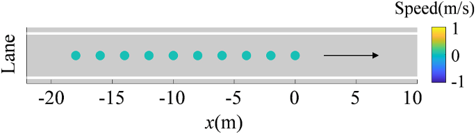
Initial distribution of vehicles
Fig. 3 
Vehicle distribution at the end of simulation
Fig. 4 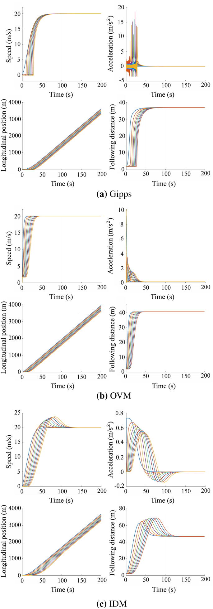
Simulation results of different following models. (Each curve represents a vehicle)
-
(2)
Deceleration and Stopping Condition
The deceleration and stopping condition is defined here as an accident ahead on the highway, and a warning sign is set at 150 m behind the accidentunder related traffic safety law [26]. The vehicle queue must decelerate to 0 before the accident happens to avoid collision. Due to the timely warning, there should be no emergency braking, so the vehicle still runs according to the car-following model. Based on the steady state at the end of the simulation in the above part, it is assumed that the first vehicle in the vehicle queue finds a warning sign at 4500 m on highway and needs to stop within 150 m. The simulation results of the three models are shown in Figs. 5 and 6.
Fig. 5 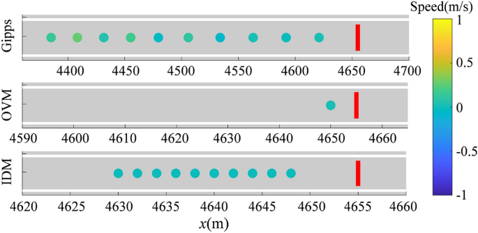
Vehicle distribution at the end of simulation
Fig. 6 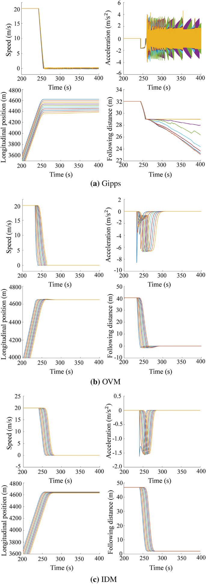
Simulation results of different following models. (Each curve represents a vehicle)
It can be seen from Fig. 5 that at the end of the simulation, the vehicle queue of the three models did not exceed the accident point (red line), but it can be found from Fig. 6a that the Gipps model does not reach stability and the acceleration is still fluctuating violently. All vehicles of OVM and IDM have reached parking status. However, it can be seen from Fig. 6b that there is not enough distance between vehicles in OVM model, resulting in the following distance reaching 0 and large acceleration during deceleration and stopping (exceeding 5 \(\mathrm{m}/{\mathrm{s}}^{2}\)). As can be seen from Fig. 6c, the IDM model ensures smooth parking and maintains a safe distance between vehicles. At the same time, the peak acceleration is well controlled, and the maximum value does not exceed 2 \(\mathrm{m}/{\mathrm{s}}^{2}\). It can be seen that Gipps model and OVM are not applicable to the above deceleration and stopping conditions, while IDM can be applied.
The simulation results of Gipps model are compared with that of OVM and IDM under the above two working conditions: (1) static starting and (2) deceleration and stopping. Only IDM realizes a more reasonable and smooth state transition in two working conditions and shows good adaptability in multiple working conditions, so the IDM car-following model is selected.


5 Lateral Constraints of the Automatic Lane-Change Generalized Model
Based on the above analysis, only IDM achieves a more reasonable and smooth state evolution. Therefore, IDM is selected as the research basis for the longitudinal constraint model. However, the lateral constraint is not considered in the IDM, which is important to the automatic lane change process. The vehicle lane-change process is the transition of two different car-following behaviors. The traditional IDM does not describe the longitudinal kinematics model of the lane change process. As shown in Fig. 1, when SV changes from lane 2 to lane 1, its lead vehicle changes from the original VFS to VFT. The difference in state between the VFS and the VFT will result in a sudden change in the output of the IDM equation, and the greater the difference, the more severe the transition. Similarly, the lane change behavior will cause a similar parameter jump to the VRS and the VRT, resulting in an unreasonable output and fluctuations to the model.
The same car-following model is used to describe the longitudinal constraint model of the vehicle before and after the lane change behavior with VFS and VFT as the following objects respectively. The SV's acceleration \(\dot{v}_{{{\text{ori}}}}\) and \(\dot{v}_{{{\text{new}}}}\) before and after the SV's lane change can be calculated according to the IDM:
Many existing studies consider the transition process of Eq. (13) to (14) to be instantaneous [27], thus causing a jump in the model output. The magnitude of the change from \((x_{{{\text{VFS}}}} - x_{{{\text{SV}}}} )\) to \((x_{{{\text{VFT}}}} - x_{{{\text{SV}}}} )\) and from \((v_{{{\text{VFT}}}} - v_{{{\text{VRT}}}} )\) to \((v_{{{\text{SV}}}} - v_{{{\text{VRT}}}} )\) determines the magnitude of the jump in the IDM output acceleration before and after the lane change. In order to visually reflect this jump, the lane change behavior is added on the basis of the simulation in Sect. 4, assuming that at 100 s, a vehicle changes from the original lane to the adjacent lane on the left. It can be seen from Fig. 7 that the lane change changes the acceleration and has a significant impact on the surrounding vehicles, which is unfavorable for the stability of the system and the vehicle ride comfort.

Traditional IDM lane change model leads to acceleration saltation
To achieve a smooth transition during the lane change process, the transition function \(\psi (\tau )\) is introduced between the state \(\dot{v}_{{{\text{new}}}}\) and \(\dot{v}_{{{\text{ori}}}}\) as Eq. (15).
\(\dot{v}_{{{\text{tar}}}}\) is the target acceleration output of the modified IDM model, and τ is the time accumulation after the start of the most recent lane change (the lane-change start time τ = 0, and τ continues to accumulate after the lane change ends). Different transition functions show varying transition characteristics. The following three different transition functions including linear function, exponential function and hyperbolic tangent function are compared and analyzed.
5.1 Linear Transition Function
The simplest transition method is a linear transition, that is, the transition from Eq. (13) to (14) is considered to be linear, and the slope is related to the transition time, and \(\psi (\tau )\) is defined as:
\(T_{{{\text{LC}}}}\) is the duration of a single-lane change process. The linear transition function is positive and smaller than 1, because \(T_{{{\text{LC}}}}\) and \(\tau \) are positive.
5.2 Exponential Transition Function
It is considered that the lane-change trend needs to be established quickly in the early stage of the lane change, so as to convey the lane change intention to the rear vehicle, and the lane-change behavior should be gentle in the later stage. Then, the exponential function of \(\psi (0) = 0\) can be used as the transition function, which is defined as follows:
\(\xi\) is the coefficient reflecting the transition speed. In order to determine \(\xi\), the stage of \(0.01 \le \psi (\tau ) \le 0.99\) is defined as the lane-change process. The stage of \(\psi (\tau ) < 0.01\) is defined as driving in the original lane. The state of \(\psi (\tau ) > 0.99\) is defined as lane change completed. Because \(\psi (\tau )\) is a monotonic function, getting:
5.3 Hyperbolic Tangent Transition Function
Inspired by the activation function of the neural network, a variant of the hyperbolic tangent function can be used to obtain a smoother transition.
\(\lambda \) and \(\gamma \) are parameters that reflect the transition speed and phase, respectively.\(\lambda \) and \(\gamma \) can be calculated as follows, with the same assumptions as the exponential transition function:
The result of Eq. (21) is:
To analyze the differences among the three transition models, they are simulated separately under the same working condition. SV’s desired speed is 35 m/s, while VFS is at a slower speed of 20 m/s, which limits the increase of the SV speed. And, VFT’s speed is 30 m/s. To improve the driving efficiency of the vehicle when the distance from the VFS is reduced to a certain value, the SV performs a free lane change from lane 2 to lane 1. This is just to analyze the similarities and differences of the three transition models without the influence of lane-change decision. It is assumed that during the entire process, VFS and VFT are running at a constant speed without changing lanes. To explain the role of the transition function, the concept of "belief lane" is introduced to indicate the weight of the lane numbers of the longitudinal restraint of the vehicle. That is, when the SV changes from lane 2 to lane 1, its longitudinal restraint is applied from VFS to VFT, and during the lane-change process, its longitudinal constraint force is considered to be jointly generated by VFS and VFT. For example, when SV is in the middle of the two lanes, 50% of the longitudinal constraint is applied by lane 1, while the others are applied by lane 2. And, the belief lane at this time is 1.5. The mathematical definition is as follows:
in which, i denotes the lane number, including the original lane and the target lane. \(\mu_{i}\) denotes the longitudinal constraint weight of the lead vehicle on i lane to the target vehicle. Herein, \(\mu_{i} = \psi (\tau )\). Referring to the lane change time [20] on the common high-speed condition, \(T_{{{\text{LC}}}}\) is determined as 4 s. SV changes lanes at the time of 30 s, that is, the SV runs according to the IDM model before 30 s and after 34 s. The simulation results are shown in Fig. 8, where (a) is the acceleration curve, (b) is the belief lane, and (c) is the longitudinal jerk degree.

Simulation results of different transition models
It can be seen that the model without transition process will have a jump in acceleration at the time of lane change. It can be seen from the degree of jerk curve in Fig. 8c that the maximum jerk degree of the model without transition reaches \(6 {\mathrm{m}/\mathrm{s}}^{3}\), which is caused by the jump of the belief lane at the beginning of the lane change. The model with the transition function realizes the continuous transition of the acceleration before and after the lane change, which directly benefits from the continuous transition of the belief lane. To compare the differences of the three transition functions, further analysis is conducted. It can be seen that the jerk degree of the linear transition model is constant, with a small amplitude jump at the beginning and end of the lane change process. The exponential transition model has a significant degree of jerk jump at the beginning of the lane change, reaching \(0.6 {\mathrm{m}/\mathrm{s}}^{3}\), and then decreases smoothly. The hyperbolic tangent transition model has a very small transition at the initial moment. A smooth transition that converges to zero is achieved by smoothing the first increase. The magnitude of the jump is only less than 1⁄2 of the linear transition model, and the peak is less than 2⁄3 of the peak of the exponential transition model.
The acceleration and jerk degree with the hyperbolic tangent transition function is close to the "perfect curve" of the smooth transition. Therefore, the transition function used herein is hyperbolic tangential transition function. Combined with the IDM model, the modified model can be expressed as Eq. (24). This model is called hybrid operating condition (mixing of car-following and lane-change conditions) IDM (HC-IDM). The model is characterized by the use of mixed conditions without the need for segmentation processing, which can achieve a smooth transition while retaining the advantages of the IDM model.
6 Simulation Result and Analysis
The automatic lane change generalized dynamic model (ALCGDM) contains IDM and HC-IDM, two kinds of car-following models, and MOBIL, lane-change decision model. The simulation environment is a two-lane highway with a speed limit of 120 km/h. There are 100 vehicles (95 cars and 5 trucks) randomly distributed in the two lanes. At the initial time, both the headway distribution and the speed distribution are in the Weibull distribution model. The headway of the intensive traffic will remain above a critical value to ensure safety. Generally, the safety headway in urban and highway working conditions is 1.5–2 s [28,29,30]. Considering that the headway on the highway is generally large and a stable following state is not reached at the beginning of the simulation, the initial headway is set as 2.5 s, which is larger than desired. And the simulation aims to verify whether the vehicle model can reach a stable state. The initial headway and vehicle speed distributions are not independent of each other. Herein, they are considered to be linearly related. The initial speed of each vehicle obeys the Weibull distribution near its expected speed. The values of related parameters are shown in Tables 2 and 3 [18, 25].
Under the excitation of the MOBIL automatic lane-change decision model, the ALCGDM can obtain the system output response, including micro comfort index, macro stability index and traffic efficiency index.
-
(1)
Micro Comfort Index
The micro comfort index is an evaluation index for an individual vehicle, and reflects the driver's ride comfort. It is usually expressed by vehicle’s acceleration or jerk degree. Figure 9 shows the acceleration, jerk degree and belief lane curves during a typical lane-change process with ①IDM + MOBIL and ②HC-IDM + MOBIL. It can be seen that when the traditional IDM model (in model combination ①) is used, the lane-change process will produce more severe acceleration jumps, resulting in a severe longitudinal jerk level. It can be seen that the jerk degree is nearly \(10 {\mathrm{m}/\mathrm{s}}^{3}\), which will significantly affect ride comfort, especially when passengers are not prepared for non-starting conditions. The reason for this excessively severe jerk degree can be seen from the belief lane curve. At the time of lane change, the belief lane changes from 1 to 2 without continuous transition. By using the HC-IDM, the acceleration jump of the lane-change process has been weakened, and the jerk degree is limited to \({2 \mathrm{m}/\mathrm{s}}^{3}\). This is directly due to the smooth and continuous transition process of the belief lane change.
Fig. 9 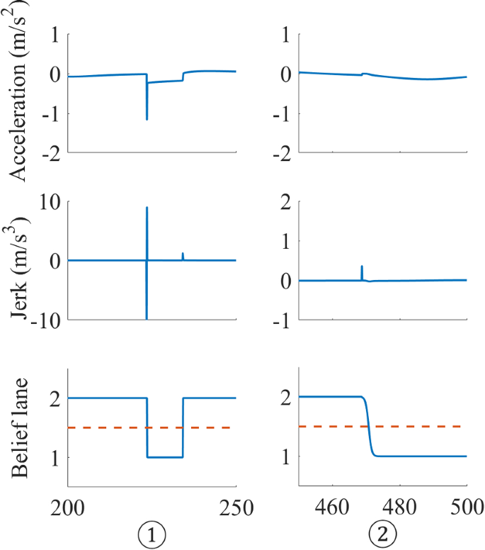
Change of vehicle status during lane change
-
(2)
Macro Stability Index
The macro stability index is an indicator of the overall traffic flow. It is usually expressed by fluctuations in the speed, acceleration, and jerk degree of the vehicle cluster. To evaluate the fluctuation of the traffic flow, the average acceleration and jerk degree of all vehicles are compared, and the results are shown in Figs. 10 and 11. It can be seen from Fig. 10 that the acceleration fluctuation of model combination ② is slighter and the peak value is smaller. In addition, it can be seen from Fig. 10b that the acceleration of the model combination ① has a sharp fluctuation, while the second has maintained a relatively flat change, which is mainly due to the introduction of the transition function in the HC-IDM. To quantitatively evaluate the magnitude of the above acceleration fluctuations, the average longitudinal jerk degree of the system is compared, and the results are shown in Fig. 11. It can be seen that even after 200 s of the simulation, the average peak jerk of model combination ① is still close to \(0.3{\mathrm{ m}/\mathrm{s}}^{3}\) (note that the absolute value of the jerk degree here is smaller because all vehicles for the entire traffic flow are averaged), and the fluctuations are severe. The average peak jerk of model ② remains at a very low level, which is less than 30% of the model combination ①. The fluctuation of the model combination ① is not conducive to the stability of the traffic flow. And, it is not conducive to the comfort of the ride from the perspective of a single vehicle (the jerk degree is expressed as the frustration of the vehicle).
Fig. 10 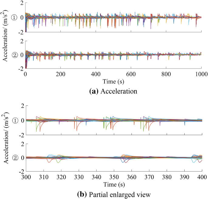
Acceleration of the traffic flow
Fig. 11 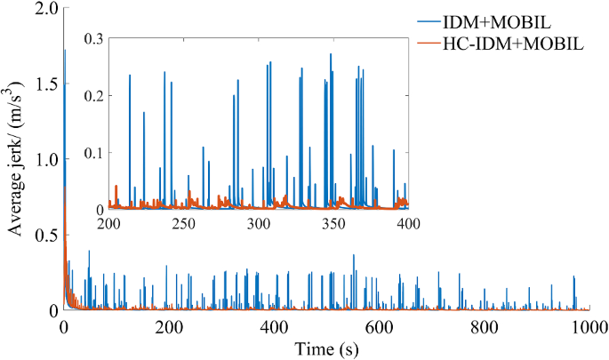
Average degree of jerk of the traffic flow
The above simulation results show that the introduction of HC-IDM addresses the parameter jump of the traditional IDM model applied in the lane-change condition. And, the performance is better during the fluctuation of traffic flow.
-
(3)
Macro Traffic Efficiency Index
The macro traffic efficiency index is an indicator of the overall traffic flow. And it is usually described by the total driving distance of the traffic flow and the average velocity of the vehicle cluster. Based on the ALCGDM, the real-time position, displacement, velocity and other output parameters of all vehicles under MOBIL lane change excitation can be obtained, as shown in Figs.12 and 13.
Fig. 12 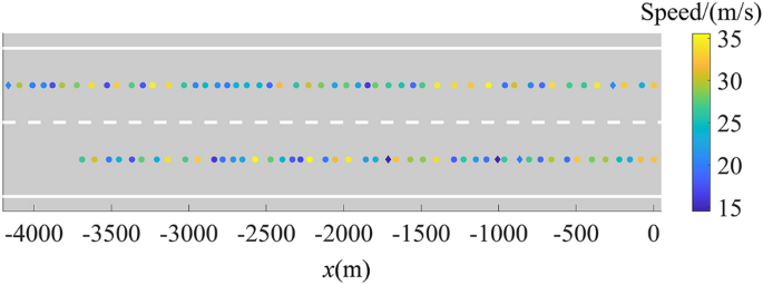
Initial vehicle velocity and spatial distribution
Fig. 13 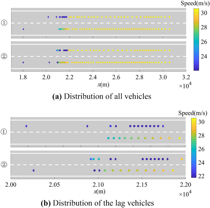
Distribution of the vehicles at the end of simulation
Figure 13 shows the spatial and velocity distribution of the vehicle flow at the end of the simulation. Compared with the initial distribution of the vehicle in Fig. 12, most of the cars (dots) have completed the overtaking of the truck in front (diamond) and obtained the ideal driving speed. If the position of \(2.2\times {10}^{4}\,\mathrm{m}\) is the dividing line, the vehicle behind the dividing line is called the lagging vehicle (as shown in Fig. 13a and Table 4). It can be seen that these vehicles are mainly trucks and cars with a lower speed. There are 14 and 13 deep blue vehicles in model combinations ① and ②, respectively. Among them, the number of slow cars (dark blue dots) behind the truck can reflect the advantages and disadvantages of the lane change strategy. As shown in Fig. 13b, there are 9 and 8 cars with low speed, respectively, in combination ① and ②. It can be seen that the HC-IDM + MOBIL model has not improved traffic efficiency significantly.
Table 4 Hysteresis Vehicle Status at the End of Simulation of Different Model Combinations In addition, the model can generate macroscopic traffic efficiency indicators, such as the total mileage of the traffic flow. The simulation results are shown in Fig. 14 and Table 5.
Fig. 14 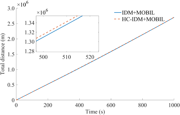
Total mileage of combination ① and ②
Table 5 Comparison of Results at the End of Simulation of Different Model Combinations Table 5 shows that the total mileage of model combinations ① and ② during the 1000s simulation are 2502.8 and 2505.2 km, respectively. And the average vehicle speeds are 28.72 and 28.77 m/s, respectively. The macroscopic traffic efficiency of the HC-IDM + MOBIL model combination is slightly higher than that of the IDM + MOBIL model, but the correction of the car-following model does not have much influence on the traffic efficiency index. And the reason for this slight improvement is that the same MOBIL lane-change decision model is used in both model combinations. Therefore, the average speed and total mileage are not improved much.


7 Conclusion
Based on theoretical mechanics, this paper proposes an automatic lane-change generalized dynamic model, promoting the evaluation of the automatic lane-change algorithm, featured by macroscopic and microscopic indicators.
To extend the application of the car-following model, IDM, from the traditional single-lane condition to the multi-lane mixed condition, the hyperbolic tangent transition function is introduced to modify the model into HC-IDM. The HC-IDM realizes the integration of the car following and lane change and avoids the state mutation and discontinuity of the existing model.
The analysis shows that the HC-IDM model has significantly improved the macro stability and micro comfort of the traffic flow compared with that using the traditional IDM model. It can be concluded that the HC-IDM can be applied to more traffic scenarios to improve the stability and comfort of traffic flow during lane change.
The current research is based on the premise of perfect automatic driving and environmental perception, that is, there are ideal assumptions. In future work, the impact of different environmental sensing sensors or vehicle networking signal characteristics on the model will be studied.
Abbreviations
- ALCGDM:
-
Automatic lane change generalized dynamic model
- IDM:
-
Intelligent driver model
- HC-IDM:
-
Hybrid operating condition IDM
- MOBIL:
-
Minimizing overall braking induced by lane changes
- OVM:
-
Optimal velocity model
References
Zheng, Z.: Recent developments and research needs in modeling lane changing. Transp. Res. Part B 60, 16–32 (2014)
Rahman, M., Chowdhury, M., Xie, Y., et al.: Review of microscopic lane-changing models and future research opportunities. IEEE Trans. Intell. Transp. Syst. 14(4), 1942–1956 (2013)
Zheng, Z., Ahn, S., Chen, D., et al.: The effects of lane-changing on the immediate follower: Anticipation, relaxation, and change in driver characteristics. Transp. Res. Part C: Emerg. Technol. 26, 367–379 (2013)
Shi, X., Wang, Z., Li, X., et al.: The effect of ride experience on changing opinions toward autonomous vehicle safety. Commun. Transp. Res. 1, 100003 (2021)
Hidas, P.: Modelling vehicle interactions in microscopic simulation of merging and weaving. Transp. Res. Part C: Emerg. Technol. 13(1), 37–62 (2005)
Sun, D., Elefteriadou, L.: Lane-Changing behavior on urban streets: an “in-vehicle” field experiment-based study. Comput.-Aided Civil Infrastruct. Eng. 27(7), 525–542 (2012)
Wouter, J., Schakel, V., Knoop, B.: Integrated lane change model with relaxation and synchronization. Transp. Res. Record J. Transp. Res. Board 23(16), 47–57 (2012)
Goñi-Ros, B., Knoop, V., Takahashi, T., et al.: Optimization of traffic flow at freeway sags by controlling the acceleration of vehicles equipped with in-car systems. Transp. Res. Part C 71, 1–18 (2016)
Lu, J., Li, Y.: Review and outlook of modeling of lane change behavior[J]. J. Transp. Syst. Eng. Inf. Technol. 17(4), 48–55 (2017)
Balal, E., Cheu, R., Sarkodie-Gyan, T.: A binary decision model for discretionary lane change move based on fuzzy inference system. Transp. Res. Part C Emerg. Technol. 67, 47–61 (2016)
Nilsson, J., Brännström, M., Coelingh, E., et al.: Lane change maneuvers for automated vehicles. IEEE Trans. Intell. Transp. Syst. 18(5), 1087–1096 (2017)
Wang, M., Hoogendoorna, S., Daamena, W., et al.: Optimal lane change times and accelerations of autonomous and connected vehicles. In: Transportation Research Board 95th Annual Meeting, TRB committee AHB45 Standing Committee on Traffic Flow Theory and Characteristics, Washington DC, 10–14 Jan 2016
Wang, M., Hoogendoorn, S., Daamen, W., et al.: Game theoretic approach for predictive lane-changing and car-following control. Transp. Res. Part C 58, 73–92 (2015)
Ulbrich, S., Maurer, M.: Towards tactical lane change behavior planning for automated vehicles. In: IEEE 18th International Conference on Intelligent Transportation Systems, 15–18 Sept 2015.
Yu, H., Tseng, H., Langari, R.: A human-like game theory-based controller for automatic lane change. Transp. Res. Part C: Emerg. Technol. 88, 140–158 (2018)
Abuamer, I., Sadat, M., Silgu, M., et al.: Analyzing the effects of driver behavior within an adaptive ramp control scheme: A case-study with ALINEA. In: IEEE International Conference on Vehicular Electronics and Safety (ICVES), pp. 109–114, 27–28 June 2017
Sadat, M., Celikoglu, H.: Simulation-based variable speed limit systems modelling: an overview and a case study on Istanbul freeways. Transp. Res. Procedia 22, 607–614 (2017)
Arne, K., Martin, T., Dirk, H.: General lane-changing model MOBIL for car-following models. Transp. Res. Record J. Transp. Res. Board 1999(1), 86–94 (2007)
Zeng, Y., Zhang, N.: Review and new insights of the car-following model for road vehicle traffic flow. In: Proceedings of the 6th International Asia Conference on Industrial Engineering and Management Innovation, vol. 1, pp. 87–96. Atlantis Press, Pairs (2016).
Jiang, R., Wu, Q., Zhu, Z.: Full velocity difference model for a car-following theory. Phys. Rev. E Stat. Nonlin. Soft. Matter. Phys. 64, 017101 (2001)
Xue, Y.: A car-following model with stochastically considering the relative velocity in a traffic flow. Acta Physica Sincia 52(11), 2750–2757 (2003)
Saifuzzaman, M., Zheng, Z.: Incorporating human-factors in car-following models: a review of recent developments and research needs. Transp. Res. Part C: Emerg. Technol. 48, 379–403 (2014)
Schakel, W., Arem, B., Netten, B.: Effects of cooperative adaptive cruise control on traffic flow stability. In: 13th International IEEE Annual Conference on Intelligent Transportation Systems, Madeira Island, Portugal, 19–22 Sept 2010.
Milanés, V., Shladover, S.: Modeling cooperative and autonomous adaptive cruise control dynamic responses using experimental data. Transp. Res. Part C Emerg. Technol. 48, 285–300 (2014)
Treiber, M., Kesting, A., Helbing, D.: Delays, inaccuracies and anticipation in microscopic traffic models. Physica A 360(1), 71–88 (2005)
Law of the People's Republic of China on Road Traffic Safety. (2004)
Yao, S., Knoop, V., Arem, B.: Optimizing traffic flow efficiency by controlling lane changes: collective, group, and user optimal. Transp. Res. Record J. Transp. Res. Board 2622, 96–104 (2017)
Kerner, B.: Introduction to modern traffic flow theory and control. Springer, Heidelberg New York, USA (2009)
Next Generation Simulation Fact Sheet, Washington, DC, USA. ops.fhwa.dot.gov/trafficanalysistools/ngsim.htm (2021). Accessed 4 Jan 2021.
Punzo, V., Borzacchiello, M., Ciuffo, B.: On the assessment of vehicle trajectory data accuracy and application to the Next Generation SIMulation (NGSIM) program data. Transp. Res. Part C Emerg. Technol. 19(6), 1243–1262 (2011)
Author information
Authors and Affiliations
Corresponding author
Ethics declarations
Conflict of interest
The authors declared no potential conflicts of interest with respect to the research, authorship, and/or publication of this article. The author(s) received no financial support for the research, authorship, and/or publication of this article.
Additional information
Academic editor: Xudong Zhang
Rights and permissions
Open Access This article is licensed under a Creative Commons Attribution 4.0 International License, which permits use, sharing, adaptation, distribution and reproduction in any medium or format, as long as you give appropriate credit to the original author(s) and the source, provide a link to the Creative Commons licence, and indicate if changes were made. The images or other third party material in this article are included in the article's Creative Commons licence, unless indicated otherwise in a credit line to the material. If material is not included in the article's Creative Commons licence and your intended use is not permitted by statutory regulation or exceeds the permitted use, you will need to obtain permission directly from the copyright holder. To view a copy of this licence, visit http://creativecommons.org/licenses/by/4.0/.
About this article

Cite this article
Wang, Y., Cao, X. & Ma, X. Evaluation of Automatic Lane-Change Model Based on Vehicle Cluster Generalized Dynamic System. Automot. Innov. 5, 91–104 (2022). https://doi.org/10.1007/s42154-021-00171-z
Received:
Accepted:
Published:
Issue Date:
DOI: https://doi.org/10.1007/s42154-021-00171-z