Comprehensive Analysis and Optimization of Dynamic Vibration-Absorbing Structures for Electric Vehicles Driven by In-Wheel Motors

Abstract

Distributed-drive electric vehicles (EVs) replace internal combustion engine with multiple motors, and the novel configuration results in new dynamic-related issues. This paper studies the coupling effects between the parameters and responses of dynamic vibration-absorbing structures (DVAS) for EVs driven by in-wheel motors (IWM). Firstly, a DVAS-based quarter suspension model is developed for distributed-drive EVs, from which nine parameters and five responses are selected for the coupling effect analysis. A two-stage global sensitivity analysis is then utilized to investigate the effect of each parameter on the responses. The control of the system is then converted into a multiobjective optimization problem with the defined system parameters being the optimization variables, and three dynamic limitations regarding both motor and suspension subsystems are taken as the constraints. A particle swarm optimization approach is then used to either improve ride comfort or mitigate IWM vibration, and two optimized parameter sets for these two objects are provided at last. Simulation results provide in-depth conclusions for the coupling effects between parameters and responses, as well as a guideline on how to design system parameters for contradictory objectives. It can be concluded that either passenger comfort or motor lifespan can be reduced up to 36% and 15% by properly changing the IWM suspension system parameters.

1 Introduction

Increasingly strict vehicle emission standards have been the main motivation for extensive research on electric vehicles (EVs), which are likely to replace the traditional internal combustion engine (ICE) in the near future [1,2,3,4]. From the perspective of system configuration, EVs can be categorized into two distinct types: centrally driven type and distributed-drive type. Compared with the centrally driven layout, the latter case incorporates an electric motor in the hub of a wheel for direct drive, and it provides numerous advantages, including more available chassis space, prompt system response and high energy efficiency [5,6,7,8,9]. In this context, distributed-drive EVs are attracting more attention from both academia and automobile industry and are also considered as the direction of current and future EVs.

However, the performance of the in-wheel motors (IWMs) used in distributed-drive EVs is restricted by the limited space inside the wheel and negative effect of the increased unsprung mass on suspension performance. Many noteworthy research projects have focused on these issues.

Current vibration mitigation algorithms used in the IWM suspension system can be categorized into four types.

• (1) Motor dynamics optimization Some algorithms have been proposed to improve the noise, vibration and harshness (NVH) performance of the IWM. Takiguchi et al. [10] and Sun et al. [11] proposed current controllers to reduce the vibration caused by the IWM.

• (2) Suspension dynamics optimization Hredzak et al. [12] used optimization algorithms to improve the system performance by optimizing the suspension component parameters. The results achieved improved ride comfort and road handling.

• (3) Active suspension control Shao et al. [13] and Wang et al. [14] used controllable suspensions for IWMs, and these can provide better results than passive systems.

• (4) Novel structure design Other than the three above-mentioned methods, the dynamic vibration absorbing system (DVAS) is also a possible candidate to mitigate vibrations caused by road excitation. The DVAS refers to a type of well-tuned spring-mass subsystem with which the main system vibration can be effectively reduced. It shows great potential for active vibration control, and a representative DVAS-based IWM suspension system is shown in Fig. 1 [15, 16].

  Fig. 1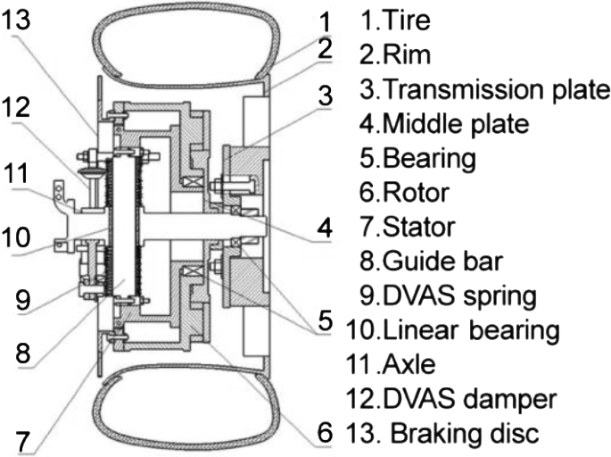

  

  Structure of the DVAS-based IWM suspension system [12]

Among these four types, the DVAS-based method is considered as a promising direction, for the reasons that it could achieve 35% improvement of ride comfort and 30% enhancement of road handling in comparison with the traditional ones [15]. However, there exists little research on how to choose DVAS parameters for conflicting objectives, and the coupling effects between system parameters and outputs have yet to be comprehensively discussed.

To understand the relationships between system parameters and responses, local sensitivity analysis (LSA) is widely used. LSA is a one-at-a-time (OAT) technique: The effect of each parameter is evaluated by calculating the partial derivative of the cost function. This method is only valid at the central point where the calculation is carried out, and cannot easily reveal the nonlinear interactions of different factors [17]. In contrast, global sensitivity analysis (GSA) uses a representative set of samples with which the full design space is explored using Monte Carlo techniques. Compared with OAT algorithm, the overall outputs of GSA methods can model the interactions of different changes to dynamic characteristics of the system. This paper adopts a two-stage evaluation strategy to solve the widely recognized computational complexity problem associated with Monte Carlo-based algorithms.

The innovations described in this paper can be summarized as follows: (1) A novel GSA algorithm is proposed to investigate the coupling effects between parameters and responses for the DVAS-IWM system, which can avoid the issues existing in conventional sensitivity analysis methods; (2) PSO is employed to provide two sets of parameters for improving ride comfort or mitigating motor vibration. The combination offers more options for varying driving conditions.

The rest of this paper is organized as follows. First, a DVAS-based IWM suspension system and road profile model are described in Sect. 2. Then, the GSA method is introduced and an in-depth analysis of the effect of system parameters is made. The PSO and the performance of the optimized system are presented in Sect. 4. A conclusion and future work are discussed in Sect. 5.

2 System Modeling

This section introduces the DVAS-based IWM suspension system and road profile generation.

2.1 The DVAS Model

The DVAS-based IWM suspension system has been well studied by previous researchers and can be regarded as a potential solution to the downsides of IWMs [15, 16]. The structure of the tire-type DVAS-based IWM suspension system is listed in Fig. 2. Its dynamics can be described by Eq. (1), as in [16].

$$\begin{array}{*{20}l} {m_{{\text{b}}} \ddot{x}_{{\text{b}}} + k_{{\text{s}}} \left( {x_{{\text{b}}} - x_{{{\text{s}}}1} } \right) + c_{{\text{s}}} \left( {\dot{x}_{{\text{b}}} - \dot{x}_{{{\text{s}}}1} } \right) = 0} \hfill \\ {m_{{\text{r}}} \ddot{x}_{{\text{r}}} + k_{{\text{b}}} \left( {x_{{\text{r}}} - x_{{\text{s}}} } \right) + c_{{\text{b}}} \left( {\dot{x}_{{\text{r}}} - \dot{x}_{{\text{s}}} } \right) = 0} \hfill \\ {m_{{\text{s}}} \ddot{x}_{{\text{s}}} + k_{{\text{d}}} \left( {x_{{\text{s}}} - x_{{{\text{s}}}1} } \right) + k_{{\text{b}}} \left( {x_{{\text{s}}} - x_{{\text{r}}} } \right)} \hfill \\ {\quad + c_{{\text{d}}} \left( {\dot{x}_{{\text{s}}} - \dot{x}_{{{\text{s}}}1} } \right) + c_{{\text{b}}} \left( {\dot{x}_{{\text{s}}} - \dot{x}_{{\text{r}}} } \right) = 0} \hfill \\ {m_{{{\text{s}}}1} \ddot{x}_{{{\text{s}}}1} + k_{{\text{t}}} \left( {x_{{{\text{s}}}1} - x_{{\text{z}}} } \right) + k_{{\text{s}}} \left( {x_{{{\text{s}}}1} - x_{{\text{b}}} } \right)} \hfill \\ {\quad + c_{{\text{s}}} \left( {\dot{x}_{{{\text{s}}}1} - \dot{x}_{{\text{b}}} } \right) + k_{{\text{d}}} \left( {x_{{{\text{s}}}1} - x_{{\text{s}}} } \right)} \hfill \\ {\quad + c_{{\text{d}}} \left( {\dot{x}_{{{\text{s}}}1} - \dot{x}_{{\text{s}}} } \right) = 0} \hfill \\ \end{array}$$

(1)

where $x_{*} ,\dot{x}_{*} {\text{ and }}\ddot{x}_{*}$ represent displacement, velocity and acceleration, respectively. The subscripts ${\text{b}},{\text{s}}_{1} ,{\text{s}},{\text{r}}$ stand for the sprung mass, total unsprung mass, stator and axle mass and rotor mass, respectively. The system parameters are listed in Table 1 [16].

Fig. 2

Structure of DVAS-based IWM suspension system

Table 1 Parameters of DVAS-based IWM suspension

2.2 Road Profile Generation

The statistical features of a real-world stochastic road profile can be represented using power spectral density (PSD). Many methods have been proposed to generate random road profiles. This paper uses harmonic superposition algorithm to model the road profile in the time domain [18]:

$$q\left( t \right) = \sum\limits_{K = 1}^{M} {\sqrt {2 \cdot G_{q} \left( {f_{{{\text{mid-}}K}} } \right) \cdot \frac{{f_{2} - f_{1} }}{M}} \sin \left( {2\uppi f_{{{\text{mid-}}K}} t + \varPhi_{K} } \right)}$$

(2)

where $q\left( t \right)$ is the generated road profile, $f_{{\text{mid-}}K}$ is the kth middle frequency, and $G_{q} \left( {f_{{\text{mid-}}K} } \right)$ represents the PSD at $f_{{\text{mid-}}K}$. Variable $\varPhi_{K}$ is an identically distributed phase over the range of $\left( {0,2\uppi } \right)$. $f_{1} ,f_{2}$ stand for the upper and lower time-domain frequency boundaries, accordingly. ISO level C was adopted as the system excitation, and the velocity was set to 60 km/h.

3 Sensitivity Analysis

This section introduces the two-step GSA and analyzes the effects each parameter has on the system response characteristics.

3.1 Introduction to Global Sensitivity Analysis (GSA)

The flowchart of the GSA-based algorithm is illustrated in Fig. 3. After both the input and output parameters are chosen for the IWM suspension system, the elementary effects analysis is carried out. The influential parameters from the first step are then fed into the second step—the GSA. Consideration of the reliance on the sensitivity index, robustness, convergence and credibility assessment is required for the careful use of GSA. Kolmogorov–Smirnov statistic approach is used as a final check that the identified sensitivity factors are comprehensive.

Fig. 3

Overall structure of the GSA

3.1.1 Elementary Effects Analysis

The purpose of the first stage is to find out the appropriate parameter which has the biggest effects on the system responses. Note that the sensitivity index generally refers to a number determined by a predefined algorithm that shows the relative sensitivity of the results to the variables. This part uses elementary effects analysis to offer a good approximation to the sensitivity index. The functionality of the elementary effect (EE) analysis is to reduce the computational cost by finding the inputs that have no effect, which are then used to calculate the sensitivity index in the second step.

For any system model $y = f\left( X \right),X = 1,2, \cdots ,k$, it is assumed that the inputs are bounded in a k-dimensional unit cube $\Omega^{k}$ with p levels. The elementary effect of any parameter $X_{i}$ is defined as:

$${\text{EE}}_{i} = \frac{{\left[ {Y\left( {X_{1} , \cdots ,X_{i - 1} ,X_{i} + \Delta , \cdots X_{k} } \right) - Y\left( {X_{1} , \cdots X_{k} } \right)} \right]}}{\Delta }$$

(3)

where $\Delta = p/\left[ {2\left( {p - 1} \right)} \right]$. It can easily be observed that the ith transformed point defined by $X + e_{i} \Delta$ is bounded inside $\Omega^{k}$, where e is a zero vector, except for its ith value, which is 1. This paper uses $p = 4$ and $\Delta = 2/3$ [17]. The average value of the ith EE is then denoted as $\mu$, which is used to evaluate the importance of each parameter. A parameter with a higher $\mu$ value represents a greater effect on a specific output. Based on the above definition, both $\mu$ and the standard deviation $\sigma$ of the ith EE can be calculated from Eq. (4), where R is the running time.

$$\begin{aligned} & \mu = \sum\limits_{j = 1}^{R} {{\text{EE}}_{i} \left( {X^{j} } \right)/R} \\ & \sigma = \sqrt {\sum\limits_{j = 1}^{R} {\left[ {{\text{EE}}_{i} \left( {X^{j} } \right) - \mu } \right]^{2} } /(R - 1)} \\ \end{aligned}$$

(4)

Note that for a complex model with interactive effects between parameters, results calculated based on values of $\mu$ may result in Type II errors, leading to the omission of influential parameters. The mean of $\mu$, denoted as $\mu^{*}$, is thus considered as the final index for EE analysis.

$$\mu^{*} = \frac{1}{R}\sum\limits_{j = 1}^{R} {\left| {{\text{EE}}_{i} \left( {X^{j} } \right)} \right|}$$

(5)

3.1.2 Global Sensitivity Analysis with the Adoption of FAST Method

GSA has become a hot topic due to its independence from the central assumption of the rest of the parameters. The widely used GSA algorithms include the Fourier amplitude sensitivity test (FAST) [19], the Morris method [20], sampling-based methods [21] and the Sobol method [22]. Among these methods, FAST is applicable to complex nonmonotonic systems and offers superior computational efficiency.

For the model used in Sect. 3.1.1, the parameters in $\Omega^{k}$ are given by:

$$\Omega^{k} = \left( {X|X_{i}^{{({\text{Min}})}} < X_{i} < X_{i}^{{({\text{Max}})}} ;i = 1, \ldots ,k} \right)$$

(6)

where $X_{i}^{{({\text{Min}})}}$ and $X_{i}^{{({\text{Max}})}}$ are the minimum and maximum values of $X_{i}$. A search function is then introduced, with which each parameter can periodically oscillate inside the space $\Omega^{k}$ at a frequency $w_{i}$. Numerous search functions have been proposed; we adopted the search function proposed by Saltelli et al. [23]:

$$X_{i} = F_{i}^{- 1} \left({\frac{1}{2} + \frac{1}{\uppi}\arcsin \left({\sin \left({w_{i} s} \right)} \right)} \right),\quad - \uppi\leqslant s\leqslant \uppi$$

(7)

where $F_{i}^{ - 1}$ is an inverse cumulative distribution function and s is a variable. It can be seen from Eq. (7) that the output is a periodic function of s. Such a function can be expanded with a Fourier series Y.

$$y = f\left( {X_{1} ,X_{2} , \ldots ,X_{k} } \right) = f(s) = A_{0} + \sum\limits_{k = 1}^{ + \infty } {\left\{ {A_{k} \cos (ks) + B_{k} \sin (ks)} \right\}}$$

(8)

where the coefficients $A_{k}$ and $B_{k}$ are:

$$\begin{aligned} & A_{0} = \frac{1}{2\uppi }\int_{ - \uppi }^{\uppi } f (s){\text{d}}s \\ & A_{k} = \frac{1}{\uppi }\int_{ - \uppi }^{\uppi } f (s)\cos (ks){\text{d}}s \\ & B_{k} = \frac{1}{\uppi }\int_{ - \uppi }^{\uppi } f (s)\sin (ks){\text{d}}s \\ \end{aligned}$$

(9)

and k is a finite integer. For an odd sample size N, k is calculated by $k \in Z = \left\{ {1, \ldots ,{{N - 1} \mathord{\left/ {\vphantom {{N - 1} 2}} \right. \kern-0pt} 2}} \right\}$. If we denote the N samples as $S = \left\{ {s_{1} ,s_{2} , \ldots ,s_{j} , \ldots ,s_{N} } \right\}$, the corresponding model outputs are calculated as:

$${\varvec{O}} = \left\{ {f\left( {s_{1} } \right),f\left( {s_{2} } \right), \ldots ,f\left( {s_{j} } \right), \ldots ,f\left( {s_{N} } \right)} \right\}$$

(10)

where $f\left( {s_{j} } \right) = f\left( {X_{1j} ,X_{2j} , \ldots ,X_{kj} } \right)$. The corresponding Fourier coefficients can therefore be expressed as

$$\begin{aligned} & A_{0} = \frac{1}{N}\sum\limits_{j = 1}^{\text{N}} f \left( {s_{j} } \right) \\ & A_{k} = \frac{2}{N}\sum\limits_{j = 1}^{\text{N}} f \left( {s_{j} } \right)\cos \left( {s_{j} K} \right) \\ & B_{k} = \frac{2}{N}\sum\limits_{j = 1}^{\text{N}} f \left( {s_{j} } \right)\sin \left( {s_{j} K} \right) \\ \end{aligned}$$

(11)

where $K = 1, \ldots ,(N - 1)/2$. The variance of a system output $V_{o}$ is then calculated and decomposed into components at the integer frequencies [24]:

$$V = \frac{1}{2}\sum\limits_{K = 1}^{(N - 1)/2} {\left( {A_{K}^{2} + B_{K}^{2} } \right)} \Rightarrow V_{i} = \sum\limits_{p} {\varLambda_{p} } w_{i}$$

(12)

where $A_{K} = \frac{1}{2}\left( {A_{K}^{2} + B_{K}^{2} } \right)(K \in {\mathbb{Z}})$ is the spectrum and p satisfies $pw_{i} \leqslant(N - 1)/2$. The result $V_{i} /V$ denotes the total variance of y.

3.2 Sensitivity Analysis Results

In this part, the simulation results of the adopted two-step GSA are discussed.

3.2.1 GSA Setting

According to Fig. 3, the first step in the GSA is to determine the candidate parameters and system responses. For the primary purpose is to investigate the effect of component parameters on an IWM suspension system, all the candidate parameters are listed in the second column of Table 2; the nominal values of these parameters are from the literature [15, 16]. For the range of both the stator and rotor masses, which are related to the power requirements and restricted by the wheel hub dimensions, the variation is set within the range from + 20 to − 20%. The range of variation of the tire stiffness, which can be viewed as a function of the tire pressure, is also set within the range from + 20 to − 20%. The parameter variations for the other parameters are set to larger ranges, for their values may significantly change as controllable suspension components are adopted.

Table 2 Candidate parameters for IWM suspension

Apart from the candidate parameter, the system responses also need to be determined; these responses, as well as the corresponding abbreviations, are tabulated in Table 3. In this paper, the first three indexes in Table 3 are widely used for the traditional suspension system evaluation, and the two latter indexes are for the IWM installed inside the wheel [16]. The reasons for these choices can be interpreted as follows: (1) SA corresponds to the vibration of the motor system, and a higher SA will result in premature fatigue failure and component damage [16], and (2) motor eccentricity represents the distance between motor and rotor, and an excessive Gap variation may result in contact with and damage to the stator body, as well as damage to the rotor.

Table 3 Investigated system responses

3.2.2 Elementary Effects

As illustrated in Fig. 3, the first step in GSA is to determine the candidate parameters and system responses. Because our primary purpose is to find which parameters among all the candidate parameters have the biggest effect, the normalized EEs of all candidate parameters on all investigated responses are presented graphically in Fig. 4. The number marked in the center of each subsquare represents the EE of the investigated parameter; a smaller number means that a parameter has a bigger effect on corresponding response.

Fig. 4

Elementary effects of the investigated parameters on system responses

Figure 4 presents the importance of each parameter to individual response through the color shade. Darker colors correspond to greater importance. Figure 4 demonstrates that the EE method can provide a qualitative description of the individual parameter effect.

Results shown in Fig. 4 reveal that the parameters of the DVAS structure have little EEs in the three traditional suspension-related indexes, which are SMA, RS and TD, and the parameters that have the biggest effect are $k_{{\text{s}}}$, $c_{{\text{s}}}$ and $k_{{\text{t}}}$, respectively. As for the two IWM responses, $c_{{\text{s}}}$ has the largest effect on SA, while the effect of suspension stiffness, DVAS stiffness and DVAS damping is also non-negotiable. The parameter $k_{{\text{b}}}$ has a dominant effect on Gap, but the other parameters affect it much less.

3.2.3 GSA Results

This section discusses the GSA results calculated by FAST (graphically presented in Fig. 5), in which the normalized sensitive indices of all candidate parameters are demonstrated for SMA, RS, TD, SA and Gap. For SMA, it is obvious that $k_{{\text{s}}}$ and $c_{{\text{s}}}$ have larger indices than the other seven candidate parameters, among which $k_{{\text{t}}}$ has the biggest effect with an index of 0.024. This phenomenon can be understood as follows: Both $k_{{\text{s}}}$ and $c_{{\text{s}}}$ are directly connected to the sprung mass, and the vibration induced by an uneven road profile is attenuated by these two suspension components. In Fig. 5b, e, both indices of $c_{{\text{s}}}$ and $k_{{\text{b}}}$ are bigger than 0.7, which means these two parameters are the most important ones for these two responses under the investigation ranges given in Table 2. The situation with TD and SA is more complex as more parameters contribute to the variation in the response variances. In the SA result, $c_{{\text{s}}}$ is the parameter that has the biggest effect, with index values of $k_{{\text{d}}}$ and $c_{{\text{d}}}$ bigger than 0.1, which means that the stator mass vibration is closely related to those components that are connected to itself. The TD results in Fig. 5c indicate that $k_{{\text{t}}}$ plays an important role, while $k_{{\text{d}}}$, $k_{{\text{s}}}$ and $c_{{\text{s}}}$ also have an impact on the range of the variation. Compared with the sensitivity analysis results for the traditional suspension structure in the study [25], in which $k_{{\text{t}}}$ and $c_{{\text{s}}}$ are the two parameters with the biggest effect on TD, it can be observed that the new parameter $c_{{\text{d}}}$, which comes from the novel DVAS, can also affect the tire deflection. Based on this observation, tire vibration can be mitigated by varying the damping coefficient of the DVAS, which provides a new perspective for improving vehicle road handling capacity with the novel DVAS. Comparison of the EE analysis results in Fig. 4 and the GSA results in Fig. 5 reveal that the EE analysis can provide a good proxy to the sensitivity analysis results.

Fig. 5

GSA results calculated by FAST: a SMA, b RS, c TD, d SA, e Gap

4 Parameter Optimization

This section introduces the DVAS-based system parameter optimization based on particle swarm optimization (PSO) and the effects that the parameter variations have on the investigated responses.

4.1 Optimization Algorithm

This section presents the parameter optimization algorithm and the effects that the parameter variations have on the investigated responses.

As the primary goal of suspension optimization is to balance system performance among multiple objectives under constraints, this paper first converts the DVAS-based system parameter design into a multiple-objective optimization problem (MOOP). For the investigated system, because a higher SA will result in premature fatigue issues as well as in component damage, we defined the objectives and the constraints of the MOOP as follows:

$$\begin{array}{*{20}l} {\hbox{min} } \hfill & {f_{1} \left( P \right) = \sigma_{{\ddot{x}_{b} }}^{{}} {\kern 1pt} ;} \hfill \\ {} \hfill & {f_{2} \left( P \right) = \sigma_{{\ddot{x}_{s1} }}^{{}} ;} \hfill \\ {{\text{subject}}\,{\text{to}}} \hfill & {3 \cdot \left| {\sigma_{\text{RS}} } \right| \le \lim \left( {\text{RS}} \right);} \hfill \\ {} \hfill & {{\kern 1pt} 3 \cdot \left| {\sigma_{\text{Gap}} } \right| \le \lim \left( {\text{Gap}} \right);} \hfill \\ {} \hfill & {3 \cdot \left| {\sigma_{\text{TD}} } \right| \le \lim \left( {\text{TD}} \right);} \hfill \\ \end{array}$$

(13)

where $P \in \Re$ is the parameters to be designed and $\sigma \left( \cdot \right)$ stands for the response RMS. In Eq. (13), $f_{1} \left( P \right)$ represents ride comfort and $f_{2} \left( P \right)$ corresponds to the vibration effects of the IWM. The three constraints are set to be the same as in [15]; i.e., $\lim \left( {\text{RS}} \right) = 0.1$ m, $\lim \left( {\text{Gap}} \right) = 0.001$ m, $\lim \left( {\text{TD}} \right) = 0.018$ m. The purpose of the following optimization can be summarized as an effort to balance both ride comfort characteristics and stator acceleration by maintaining RS, Gap and TD within the constraints.

This paper describes the global sensitivity of the parameters listed in Table 2, in which both the mass and component parameters of the suspension are considered to be variables. In the following parts, we will optimize the system according to the MOOP defined in Eq. (13). Because the masses are determined once the system configuration is fixed, we assume the mass is constant and only the suspension components, that is, $k_{{\text{d}}} ,c_{{\text{d}}} ,k_{{\text{s}}} ,c_{{\text{s}}} ,c_{{\text{b}}} ,k_{{\text{b}}}$ and the ranges defined in Table 2, are to be optimized by PSO. The PSO approach was proposed in the early 1990s [26]. It originated from animal social behavior, as a stylized representation of the movement of flocks of birds or schools of fish. The candidate solution, which is called a particle, moves inside the search space to obtain the best solution.

4.2 Optimization Results

For the MOOP defined in Eq. (13), both SMA and SA are regarded as the responses to be optimized. In this part, we provide two-parameter sets for improving ride comfort (SMA-oriented) or mitigating IWM vibrations (SA-oriented). The PSO results for the six parameters are given in Table 4.

Table 4 Parameter optimization results

It can be seen from Table 4 that all six parameters for both cases are within the range defined in the last column. Based on the two-parameter sets, the simulation results for a vehicle driving on a level but nonsmooth level C road at 60 km/h are given in Figs. 6, 7 and Table 5. The passive responses in the plots and tables correspond to the IWM suspension system without DVAS, and the parameters are the same as in [15]. The RMS comparisons (given in Table 5) show that the emphasis in the design of the IWM suspension system characteristics can be changed by varying the weights of the objective functions. The variations in the six parameters result in a 15% change in SMA (from 0.544 to 0.627 m/s²) and a 36% change in SA (from 3.67 to 5.02 m/s²). Another observation from Table 5 is that SMA and SA are conflicting objectives: They cannot be improved simultaneously.

Fig. 6

Comparisons of different systems in time domain

Fig. 7

Comparisons of different systems in frequency domain

Table 5 Comparisons of system performance

The comparison in the frequency domain is shown in Fig. 7. The comparison results for SMA show that the SMA-oriented parameter set can improve ride comfort, especially in 4–8 Hz frequency range, which is the most sensitive frequency range for the human body. The SA comparison results show that the performance of the SA-oriented dataset is superior to that of the others, especially in the 8–12 Hz range.

Based on the above simulation results, two conclusions can be drawn for parameter tuning. (1) The most important parameters for SMA are the vehicle suspension parameters, that is, k_s and c_s. Smaller k_s and c_s are beneficial to ride comfort improvement. (2) Tuning on an SA-oriented system is more complex than on an SMA-oriented system, as multiple parameters have a non-negligible effect on SA. A bigger c_s value and smaller k_d and c_d values will be helpful for SA reduction.

In summary, it can be concluded that the changes of IWM suspension system parameters can achieve different system characteristic objectives.

5 Conclusions

This paper presents theoretical and numerical simulation studies of the coupling effects between IWM and suspension system parameters and characterizes responses to parameter changes in IWM-driven EVs. Nine variable system parameters and five dynamic-related responses were selected based on the DVAS-based IWM suspension model, and a two-stage GSA-based algorithm was used to investigate the effect that each parameter had on the responses. In this algorithm, the EE of each individual parameter was first estimated to reduce the calculation complexity. GSA was then used to calculate the sensitivity indices. It was found that the damping between the rotor and stator was effect-free, while the other parameters had prominent influences on system responses. The results of this analysis showed that EE analysis could provide a good proxy for the overall sensitivity analysis result and a guideline on how to change system parameters for desired system responses. Finally, PSO was adopted to optimize the system for the engineer’s choice of either improved ride comfort or mitigation of IWM vibrations. Numerical simulation results showed that SMA and SA are conflicting objectives, and parameter changes can improve SMA and SA by up to 15% and 36%, respectively.

Future research will focus on:

• (1) Investigation of the parameter sensitivities for a full vehicle model, considering longitudinal and lateral dynamics.

• (2) Research on adaptive DVAS-based IWM suspension systems based on the optimization results.

References

Hu, C., Wang, Z., Taghavifar, H., et al.: MME-EKF-based path-tracking control of autonomous vehicles considering input saturation. IEEE Trans. Veh. Technol. 68(6), 5246–5259 (2019)
Huang, Y., Li, B., Li, S.E., et al.: Guest editorial: recent advancements on electrified, low emission and intelligent vehicle systems. IET Intell. Transp. 13(1), 1–2 (2019)
Jalali, M., Hashemi, E., Khajepour, A., et al.: Integrated model predictive control and velocity estimation of electric vehicles. Mechatronics 46(2), 84–100 (2017)
Tang, X., Yang, W., Hu, X.: A novel simplified model for torsional vibration analysis of a series–parallel hybrid electric vehicle. Mech. Syst. Signal Process. 85(3), 329–338 (2017)
Hu, C., Wang, Z., Qin, Y., et al.: Lane keeping control of autonomous vehicles with prescribed performance considering the rollover prevention and input saturation. IEEE Trans. Intell. Transp. Syst. (2019). https://doi.org/10.1109/TITS.2019.2924937
Hu, C., Wang, R., Yan, F., et al.: Differential steering based yaw stabilization using ISMC for independently actuated electric vehicles. IEEE Trans. Intell. Transp. Syst. 19(3), 627–638 (2017)
Zhao, W., Wang, Y., Wang, C.: Multidisciplinary optimization of electric-wheel vehicle integrated chassis system based on steady endurance performance. J. Clean. Prod. 186(11), 640–651 (2018)
Zhao, W., Qin, X., Wang, C.: Yaw and lateral stability control for four-wheel steer-by-wire system. IEEE Trans. Mechatron. 23(2), 2628–2637 (2018)
Peng, H., Wang, W., Xiang, C., et al.: Torque coordinated control of four in-wheel motor independent-drive vehicle with consideration of the safety and economy. IEEE Trans. Veh. Technol. (2019). https://doi.org/10.1109/TVT.2019.2935617
Takiguchi, M., Sugimoto, H., Kurihara, N., et al.: Acoustic noise and vibration reduction of SRM by elimination of third harmonic component in sum of radial forces. IEEE Trans. Power Appar. Syst. 30(2), 1–9 (2015)
Sun, W., Li, Y., Huang, J., et al.: Vibration effect and control of in-wheel switched reluctance motor for electric vehicle. J. Sound Vib. 338(2), 105–120 (2015)
Hredzak, B., Gair, S., Eastham, J.F.: Control of an EV drive with reduced unsprung mass. IEEE Proc. Electr. Power Appl. 145(7), 600–606 (1998)
Shao, X., Naghydy, F., Du, H., et al.: Coupling effect between road excitation and an in-wheel switched reluctance motor on vehicle ride comfort and active suspension control. J. Sound Vib. 443(5), 683–702 (2019)
Wang, R., Hui, J., Yan, F., et al.: Optimization and finite-frequency H∞ control of active suspensions in in-wheel motor driven electric ground vehicles. J. Franklin Inst. 352(11), 468–484 (2015)
Qin, Y., He, C., Shao, X., et al.: Vibration mitigation for in-wheel switched reluctance motor driven electric vehicle with dynamic vibration absorbing structures. J. Sound Vib. 419(4), 249–267 (2018)
Xu, B., Xiang, C., Qin, Y., et al.: Semi-active vibration control for in-wheel switched reluctance motor driven electric vehicle with dynamic vibration absorbing structures: concept and validation. IEEE Access 6, 60274–60285 (2018)
Saltelli, A., Ratto, M., Andres, T., et al.: Global Sensitivity Analysis: The Primer. Wiley, Hoboken (2008)
Qin, Y., Rath, J., Hu, C., et al.: Adaptive nonlinear active suspension control based on a robust road classifier with a modified super-twisting algorithm. Nonlinear Dyn. 97(3), 2425–2442 (2019)
McRae, G., Tilden, J., Seinfeld, J.: Global sensitivity analysis—a computational implementation of the Fourier amplitude sensitivity test (FAST). Comp. Adv. Chem. Eng. 6(11), 15–25 (1982)
Morris, M.: Factorial sampling plans for preliminary computational experiments. Technometrics 33(2), 161–174 (1991)
Lu, Y., Mohanty, S.: Sensitivity analysis of a complex, proposed geologic waste disposal system using the Fourier amplitude sensitivity test method. Reliab. Eng. Syst. Saf. 72(6), 275–291 (2001)
Sobol, I.M.: Sensitivity estimates for nonlinear mathematical models. Math. Modell. 1, 407–414 (1993)
Saltelli, A., Tarantola, S., Chan, K.S.: A quantitative model-independent method for global sensitivity analysis of model output. Technometrics 41(2), 39–56 (1999)
Cukier, R., Levine, H., Shuler, K.: Nonlinear sensitivity analysis of multiparameter model systems. J. Comput. Phys. 26(7), 1–42 (1978)
Qin, Y., Wang, Z., Xiang, C., et al.: A novel global sensitivity analysis on the observation accuracy of the coupled vehicle model. Veh. Syst. Dyn. 57(10), 1445–1466 (2019)
Kennedy, J., Eberhart, R.: Particle swarm optimization (PSO). In: Proceedings of IEEE International Conference on Neural Networks, Perth, Australia, pp. 1942–1948 (1995)
Funding
This study was supported by Young Scientists Fund (Grant No. 51805028) and Postdoctoral Research Foundation of China (Grant No. BX201600017).
Author information
Authors and Affiliations
Corresponding author
Ethics declarations
Conflict of interest
On behalf of all authors, the corresponding authors state that there is no conflict of interest.
Rights and permissions
Open Access This article is distributed under the terms of the Creative Commons Attribution 4.0 International License (http://creativecommons.org/licenses/by/4.0/), which permits unrestricted use, distribution, and reproduction in any medium, provided you give appropriate credit to the original author(s) and the source, provide a link to the Creative Commons license, and indicate if changes were made.
About this article
Cite this article
Qin, Y., Wang, Z., Yuan, K. et al. Comprehensive Analysis and Optimization of Dynamic Vibration-Absorbing Structures for Electric Vehicles Driven by In-Wheel Motors. Automot. Innov. 2, 254–262 (2019). https://doi.org/10.1007/s42154-019-00079-9
Received:
Accepted:
Published:
Issue Date:
DOI: https://doi.org/10.1007/s42154-019-00079-9