Persistent cup product structures and related invariants

Abstract

One-dimensional persistent homology is arguably the most important and heavily used computational tool in topological data analysis. Additional information can be extracted from datasets by studying multi-dimensional persistence modules and by utilizing cohomological ideas, e.g. the cohomological cup product. In this work, given a single parameter filtration, we investigate a certain 2-dimensional persistence module structure associated with persistent cohomology, where one parameter is the cup-length $\ell \ge 0$ and the other is the filtration parameter. This new persistence structure, called the persistent cup module, is induced by the cohomological cup product and adapted to the persistence setting. Furthermore, we show that this persistence structure is stable. By fixing the cup-length parameter $\ell$, we obtain a 1-dimensional persistence module, called the persistent $\ell$-cup module, and again show it is stable in the interleaving distance sense, and study their associated generalized persistence diagrams. In addition, we consider a generalized notion of a persistent invariant, which extends both the rank invariant (also referred to as persistent Betti number), Puuska’s rank invariant induced by epi-mono-preserving invariants of abelian categories, and the recently-defined persistent cup-length invariant, and we establish their stability. This generalized notion of persistent invariant also enables us to lift the Lyusternik-Schnirelmann (LS) category of topological spaces to a novel stable persistent invariant of filtrations, called the persistent LS-category invariant.

1 Introduction

Persistent Homology in TDA In Topological Data Analysis (TDA), one studies the evolution of homology across a filtration of spaces, called persistent homology (Frosini 1990, 1992; Robins 1999; Zomorodian and Carlsson 2005; Cohen-Steiner et al. 2007; Edelsbrunner and Harer 2008; Carlsson 2009, 2020). Persistent homology is able to extract both the time when a topological feature (e.g. a component, loop, cavity) is ‘born’ and the time when it ‘dies’. The collection of these birth-death pairs (real intervals) constitute the barcode, also called the persistence diagram, of the filtration (depending on the manner in which they are visualized).

Cohomology Rings in TDA In the case of cohomology, which is dual to the case of homology for a given field K, one studies linear functions on (homology) chains, known as cochains. Cohomology has a graded ring structure, inherited from the cup product operation on cochains, denoted by $\smile :{\textbf{H}}^p( X) \times {\textbf{H}}^q( X)\rightarrow {\textbf{H}}^{p+q}( X)$ for a space X and dimensions $p,q\ge 0$; see (Munkres 1984, Sec.  48 and Sec.  68) and Hatcher (2000, Ch. 3, Sec. 3.D). This makes the cohomology ring a richer structure than homology (vector spaces).

Persistent cohomology has been studied in de Silva et al. (2011a), de Silva et al. (2011b), Dłotko and Wagner (2014), Bauer (2021), Kang et al. (2021), without exploiting the ring structure induced by the cup product. Works which do attempt to exploit this ring structure include (González Díaz and Real Jurado 2003; Kaczynski et al. 2010) in the standard case and Huang (2005), Yarmola (2010), Aubrey (2011), Herscovich (2018), Belchí and Stefanou (2021), Contreras and Perea (2021), Lupo et al. (2022), Contessoto et al. (2022) at the persistent level.

In Huang (2005), the author applies the persistence algorithm toward calculating a set of invariants related to the cup products in the cohomology ring of a space. In Yarmola (2010), the author studies an algebraic substructure of the cohomology ring. In Contreras and Perea (2021), the authors study a persistence based approach for differentiating quasi-periodic and periodic signals which is inherently based on cup products.

In Aubrey (2011), the author develops a setting for persistent characteristic classes and constructs algorithms for (i) finding the Poincare Dual to a homology class, (ii) decomposing cohomology classes and (iii) deciding when a cohomology class is a Steenrod square. In Lupo et al. (2022) the authors establish the notion of persistent Steenrod modules by incorporating the Steenrod square operation into the persistence computational pipeline, and they implement an algorithm to compute the barcode of persistent Steenrod modules (Lupo et al. 2021).

Assuming an embedding of a simplicial set into ${\mathbb {R}}^n$, the author of Herscovich (2018) studies a notion of barcodes (together with a suitable extension of the bottleneck distance) which absorb information from a certain $A_\infty$-algebra structure on persistent cohomology. In Belchí and Stefanou (2021), the authors study the structure and stability of a family of barcodes that absorb information from an $A_\infty$-coalgebra structure on persistent homology. See also Belchí and Murillo (2015).

In Ginot and Leray (2019), the authors study several interleaving-type distances on persistent cohomology by considering different algebraic structures (including the natural ring structure) and study the stability of the persistent cohomology for filtrations.

In our previous joint work with Contessoto et al. (2022), we tackled the question of quantifying the evolution of the cup product structure across a filtration through introducing a polynomial-time computable invariant which is induced from the notion of cup-length: the maximal number of cocycles (in dimensions 1 and above) having non-zero cup product. We call this invariant the persistent cup-length invariant, and we identify a tool - the persistent cup-length diagram (associated to a family of representative cocycles $\varvec{\sigma }$ of the barcode) as well as a polynomial-time algorithm to compute it. In Sect. 2.3, we recall and provide more details for the mathematical results in Contessoto et al. (2022). Readers interested in the algorithmic part should still refer to the original paper (Contessoto et al. 2022).

The goal of this paper is to develop more general notions of persistent invariants that can extract additional information from the cup product operation than just the persistent cup-length invariant, including the persistent LS-category (see Sect. 2.4) and the persistent cup modules (see Sect. 4).

Some invariants related to the cup product An invariant in standard topology is a quantity assigned to a given topological space that remains invariant under a certain class of maps. This invariance helps in discovering, studying, and classifying properties of spaces when the class of maps is that of homotopy equivalences. Beyond Betti numbers, examples of classical invariants are: the Lyusternik-Schnirelmann category (LS-category) of a space X, defined as the minimal integer $k\ge 1$ such that there is an open cover $\{U_i\}_{i=1}^k$ of X such that each inclusion map $U_i\hookrightarrow X$ is null-homotopic, and the cup-length invariant, which is the maximum number of positive-degree cocycles having non-zero cup product. While being relatively more informative, the LS-category is difficult to compute (Cornea et al. 2003), and the rational LS-category is known to be NP-hard to compute (Lechuga and Murillo 2000).¹ The cup-length invariant, as a lower bound of the LS-category (Rudyak 1999a, b), serves as a computable estimate for the LS-category. Another well known invariant which can be estimated through the cup-length is the so-called topological complexity (Smale 1987; Farber 2003; Sarin 2017).

Our contributions Let denote the category of (compactly generated weak Hausdorff) topological spaces.² Throughout the paper, by a (topological) space we refer to an object in , and by a persistent space we mean a functor from the poset category $({\mathbb {R}},\le )$ to . A filtration (of spaces) is an example of a persistent space where the transition maps are given by inclusions. This paper considers only persistent spaces with a discrete set of critical values. In addition, all (co)homology groups are assumed to be taken over a field $K$. We denote by the set of intervals of type $\omega$, where $\omega$ can be any one of the four types: open-open, open-closed, closed-open and closed-closed. Results in this paper apply to all four situations, so for simplicity of notation, we state our results only for closed-closed intervals and omit $\omega$ unless otherwise stipulated.

Let be a poset category (e.g., or ${\mathbb {N}}^{\infty ,\infty }$) with a partial order $\le$. Let be the opposite category of , i.e. a poset category on equipped with the converse (or dual) relation $\ge$.³ In Sect. 2, for any given category , we define the -valued categorical invariants to be maps assigning values to both objects and morphisms in , such that ${\textbf{I}}({\text {id}}_X)={\textbf{I}}(X)$ for all and ${\textbf{I}}(g\circ f)\le \min \{{\textbf{I}}(f),{\textbf{I}}(g)\}$ for any $f:X\rightarrow Y$, $g:Y\rightarrow Z$ in ; see Definition 2.5 and Proposition 2.8. Compared with classical invariants, which are usually only defined on the objects of the underlying category, categorical invariants are also defined on the morphisms. Notice that categorical invariants are always invariant under isomorphisms (see Remark 2.6).

Here we are abusing the name ‘invariant’, and the standard notion of invariant is more closely related to what we call epi-mono invariant, i.e. invariants that are non-increasing under regular epimorphisms and non-decreasing under monomorphism.

The categorical invariants from Definition 2.5 can be seen as a generalization of the notion of epi-mono invariant mentioned in Example 2.9 and of other invariants that appeared in TDA literature (see Sect. 2.2.1 for a detailed comparison):

• For an abelian category, the notion of epi-mono-respecting pre-orders on of Puuska (2020, Defn. 3.2) is equivalent to the restriction of our notion of epi-mono invariant to abelian categories.

• For any category, the notion of categorical persistence function of Bergomi et al. (2020, Defn. 3.2) is a categorical invariant satisfying an additional inequality.

• For a regular category, an epi-mono invariant is a special case of a categorical invariant (see 2.2.1 for the details). Examples of epi-mono invariants, include rank functions of Bergomi et al. (2020, Defn. 2.1) and amplitudes of Giunti et al. (2021, Defn. 3.1).

The persistent LS-category invariant, which we introduce in this work, cannot be realized as an invariant of the above types, making our notion of categorical invariant a non-trivial generalization.

Given any persistent object, i.e. a functor , a categorical invariant ${\textbf{I}}$ gives rise to a persistent (categorical) invariant defined as the functor sending each interval [a, b] to the ${\textbf{I}}$-invariant of the transition map $f_a^b$, cf. Definition 2.7.⁴ For example, the well-known rank invariant (Carlsson and Zomorodian 2007, Defn. 11) of a persistent module is a persistent invariant induced by the dimension map defined by sending each vector space to its dimension and each linear map to the dimension of its image. Here denotes the category of finite-dimensional vector spaces over a given field K.

In Sect. 2.3, we realize the cup-length invariant as a categorical invariant by defining the cup-length of a map to be the cup-length of its image. We then lift the cup-length invariant to a persistent invariant: for a persistent space with $t\mapsto X_t$, the persistent cup-length invariant of $X_{\bullet }$, see Definition 2.14, is defined as the functor from to $({\mathbb {N}},\ge )$ of non-negative integers, which assigns to each interval [a, b] the cup-length of the image ring ${\text {im}}\big ({\textbf{H}}^*( X_b) \rightarrow {\textbf{H}}^*( X_a) \big )$. See also (Contessoto et al. 2022, Sec. 2) for details.

In Sect. 2.4, we recall the notion of the LS-category of a map first introduced in Fox (1941) and more carefully studied in Berstein and Ganea (1962, Defn. 1.1), and see that the LS-category is a categorical invariant of topological spaces. We define the persistent LS-category invariant of a persistent space $X_{\bullet }$ to be the function of $X_{\bullet }$ assigning to each interval [a, b] the LS-category of the transition map $X_a\rightarrow X_b$; see Definition 2.31. In Proposition 2.32, we prove that in analogy with the standard fact that cup-length is a lower bound for the LS-category their persistent versions also satisfy that inequality: for any interval [a, b],

$$\begin{aligned} {\textbf{cup}}(X_{\bullet })([a,b])\le {\textbf{cat}}(X_{\bullet })([a,b]). \end{aligned}$$

See Fig. 1 for examples of the persistent cup-length invariant and the persistent LS-category invariant. Although the latter invariant is pointwisely bounded below by the former, the latter is not necessarily stronger in terms of distinguishing topological filtrations; see Example 2.34.

Fig. 1

The persistent invariants ${\textbf{I}}({\text {VR}}\left( {\mathbb {T}}^2\vee {\mathbb {S}}^3\right) )$ (left) and ${\textbf{I}}({\text {VR}}\left( ({\mathbb {S}}^1\times {\mathbb {S}}^2)\vee {\mathbb {S}}^1\right) )$ (right), respectively, for ${\textbf{I}}={\textbf{cup}}$ or ${\textbf{cat}}$. Here, $\zeta _2=\arccos (-\tfrac{1}{3})\approx 0.61\pi$, $\zeta _3=\arccos (-\tfrac{1}{4})\approx 0.58\pi$ and gray regions means undetermined values. See Example 4.2

In Sect. 3, we establish stability results for persistent invariants. We first prove that the erosion distance $d_{\textrm{E}}$ between persistent invariants is bounded above by the interleaving distance $d_{\textrm{I}}$ between the underlying persistent objects (see Sect. 3.1):

Theorem 1

($d_{\mathrm I}$-stability of persistent invariants) Let be a category, and let be a categorical invariant of . The persistence ${\textbf{I}}$-invariant is 1-Lipschitz stable: for any ,

$$\begin{aligned} d_{\textrm{E}}({\textbf{I}}(F_\bullet ),{\textbf{I}}(G_\bullet ))\le d_{\mathrm I}(F_\bullet ,G_\bullet ). \end{aligned}$$

In Sect. 3.2, for the case of topological spaces, we consider categorical invariants that preserve weak homotopy equivalences, and we strengthen the above stability result by replacing $d_{\textrm{I}}$ with the homotopy-interleaving distance $d_{\textrm{HI}}$ introduced by Blumberg and Lesnick (2017, Definition 3.6). Following the fact that $d_{\textrm{HI}}$ is stable under the Gromov–Hausdorff distance $d_{\textrm{GH}}$ between metric spaces (see Proposition 3.4), we also obtain stability of such categorical invariants in the Gromov–Hausdorff sense:

Theorem 2

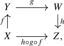
(Homotopical stability) Let ${\textbf{I}}$ be a categorical invariant of topological spaces satisfying the condition that for any maps $X\xrightarrow {f}Y\xrightarrow {g}Z\xrightarrow {h}W$ where g is a weak homotopy equivalence, ${\textbf{I}}(g\circ f)={\textbf{I}}(f)$ and ${\textbf{I}}(h\circ g)={\textbf{I}}(h)$. Then, for two persistent spaces , we have

$$\begin{aligned} d_{\textrm{E}}({\textbf{I}}(X_{\bullet }),{\textbf{I}}(Y_\bullet ))\le d_{\textrm{HI}}(X_{\bullet },Y_\bullet ). \end{aligned}$$

(1)

For the Vietoris-Rips filtrations ${\text {VR}}_\bullet (X)$ and ${\text {VR}}_\bullet (Y)$ of compact metric spaces X and Y, we have

$$\begin{aligned} d_{\textrm{E}}\left( {\textbf{I}}\left( {\text {VR}}_\bullet (X)\right) ,{\textbf{I}}\left( {\text {VR}}_\bullet (Y)\right) \right) \le 2\cdot d_{\textrm{GH}}(X,Y). \end{aligned}$$

(2)

We apply the above theorem to show that the persistent cup-length invariant and the persistent LS-category are stable:

Corollary 1.1

(Homotopical stability of ${\textbf{cup}}(\cdot )$) For persistent spaces , the persistent cup-length invariant ${\textbf{cup}}(\cdot )$ satisfies Eqs. (1) and (2).

Corollary 1.2

(Homotopical stability of ${\textbf{cat}}(\cdot )$) For persistent CW complexes , the persistent LS-category ${\textbf{cat}}(\cdot )$ satisfies Eqs. (1) and (2).

Notice that the persistent cup-length invariant and persistent LS-category invariant are comparable in the sense that neither invariant is stronger than the other (see Example 2.34), similar to the static case (see Example 2.30).

Through several examples, we show that the persistent cup-length (or LS-category) invariant helps in discriminating filtrations when persistent homology fails to or has a relatively weak performance in doing so, e.g. (Contessoto et al. 2022, Ex. 13). Also, in Example 3.6, we specify suitable metrics on the torus ${\mathbb {T}}^2$ and on the wedge sum ${\mathbb {S}}^1 \vee {\mathbb {S}}^2 \vee {\mathbb {S}}^1$, and compute the erosion distance between their persistent cup-length (or LS-category) invariants and apply Theorem 2 to obtain a lower bound $\tfrac{\pi }{6}$ for the Gromov–Hausdorff distance between them ${\mathbb {T}}^2$ and ${\mathbb {S}}^1 \vee {\mathbb {S}}^2 \vee {\mathbb {S}}^1$ (see Proposition 3.7).⁵ We also verify that the interleaving distance between the persistent homology of these two spaces is at most $\tfrac{3}{5}$ of the bound obtained from persistent cup-length (or LS-category) invariants. See Remark 3.8.

In Sect. 4, for a given persistent space $X_{\bullet }$ and any $\ell \in {\mathbb {N}}^+$, we study the $\ell$-fold product $({\textbf{H}}^{ + }(X_{\bullet }))^{\ell }$ of the persistent (positive-degree) cohomology ring, via the notion of flags of vector spaces. A flag (of vector spaces) means a non-increasing sequence of vector spaces connected by inclusions,⁶ e.g. $V_1\supseteq V_2\supseteq \cdots$. A flag is said to have finite depth if there is some n such that $V_n=0$ (as a consequence, $V_k=0$ for all $k\ge n$). Similarly, we call a non-increasing sequence of graded vector spaces connected by degree-wise inclusions to be a graded flag:

$$\begin{aligned} \bigoplus _{p\ge 1} V^{p}_1 \supseteq \bigoplus _{p\ge 1} V^{p}_2 \supseteq \cdots \supseteq \bigoplus _{p\ge 1} V^{p}_\ell \supseteq \cdots . \end{aligned}$$

For a topological space X, we define $\Phi ( X)$ to be the graded flag induced by $\ell$-fold product $({\textbf{H}}^{ + }( X))^\ell$ for all $\ell \in {\mathbb {N}}^+$:

$$\begin{aligned} \Phi ( X):=\, {\textbf{H}}^{ + }( X)\supseteq ({\textbf{H}}^{ + }( X))^{ 2}\supseteq ({\textbf{H}}^{ + }( X))^{3}\supseteq \cdots . \end{aligned}$$

Let and be the category of finite-depth flags and finite-depth graded flags, respectively. For a persistent space $X_{\bullet }$, we have the persistent graded flag with $t\mapsto \Phi ( X_t)$, and we call it the persistent cup module of $X_{\bullet }$. Indeed, the persistent cup module can be described via the following commutative diagram: for any $t\le t'$,

The above diagram suggests that the persistent cup module $\Phi (X_{\bullet })$ has the structure of a 2D persistence module, which we still denote as $\Phi (X_{\bullet })$ but view as a functor Two-dimensional persistent modules have wild types of indecomposables in most cases (Leszczyński 1994; Leszczyński and Skowroński 2000; Bauer et al. 2020), making them difficult to study (see Sect. 4.4 for details). Therefore, in Sect. 4.1, we concentrate on studying $\Phi (X_{\bullet })$ as a persistent graded flag, and taking the point of view of generalized persistent diagrams (Patel 2018, Definition 7.1).

Flags can be completely characterized by a non-increasing sequence of integers, where each integer is the dimension of the corresponding vector space (see Proposition 4.1). We call such non-increasing sequence of integers the dimension of a flag, and write it as

$$\begin{aligned} {\textbf{dim}}(V_1\supseteq V_2\supseteq \cdots ):=\big ({\textbf{dim}}(V_1),{\textbf{dim}}(V_2),\dots \big ). \end{aligned}$$

We define the rank invariant of flags as the map sending each flag to its dimension and each flag morphism to the dimension of its image; see Definition 4.7. This invariant is clearly a (${\mathbb {N}}^\infty$-valued) categorical invariant and thus can be lifted to a persistent invariant. Similarly, we define the dimension of a graded flag, to be a matrix such that each row is the dimension of the flag in the corresponding degree: The dimension ${\textbf{dim}}\left( \bigoplus _{p\ge 1} V^{p}_1 \supseteq \bigoplus _{p\ge 1} V^{p}_2 \supseteq \cdots \supseteq \bigoplus _{p\ge 1} V^{p}_\ell \supseteq \cdots \right)$ is defined as

$$\begin{aligned} \begin{pmatrix} {\textbf{dim}}(V_1^1) &{}\quad {\textbf{dim}}(V_2^1) &{}\quad \cdots &{}\quad {\textbf{dim}}(V_\ell ^1) &{}\quad \cdots \\ {\textbf{dim}}(V_1^2) &{}\quad {\textbf{dim}}(V_2^2) &{}\quad \cdots &{}\quad {\textbf{dim}}(V_\ell ^2) &{}\quad \cdots \\ \cdots &{}\quad \cdots &{}\quad \cdots &{} \quad \cdots &{} \quad \cdots \\ {\textbf{dim}}(V_1^p) &{}\quad {\textbf{dim}}(V_2^p) &{} \quad \cdots &{} \quad {\textbf{dim}}(V_\ell ^p) &{}\quad \cdots \\ \cdots &{}\quad \cdots &{}\quad \cdots &{}\quad \cdots &{}\quad \cdots \end{pmatrix}, \end{aligned}$$

The rank invariant of graded flags is defined similar to the non-graded case and will also be denoted as ${\textbf{rk}}$. See Fig. 2.

Fig. 2

Rank invariants ${\textbf{rk}}\left( \Phi ({\text {VR}}\left( {\mathbb {T}}^2\vee {\mathbb {S}}^3\right) )\right)$ (left) and ${\textbf{rk}}\left( \Phi ({\text {VR}}\left( ({\mathbb {S}}^1\times {\mathbb {S}}^2)\vee {\mathbb {S}}^1\right) )\right)$ (right) of persistent cup modules (up to degree 3) arising from Vietoris-Rips filtrations of ${\mathbb {T}}^2\vee {\mathbb {S}}^3$ and $({\mathbb {S}}^1\times {\mathbb {S}}^2)\vee {\mathbb {S}}^1$, respectively. See Example 4.2

We show that the erosion distance $d_{\textrm{E}}$ between persistent cup modules is stable under the homotopy-interleaving distance $d_{\textrm{HI}}$ between persistent spaces, which is a consequence of Theorem 1. In addition, the stability of persistent cup modules improves the stability of the persistent cup-length invariant. Recall from Chazal et al. (2016) that a standard persistence module is $\textrm{q}$-tame if it satisfies the condition that ${\textbf{rk}}(M_t\rightarrow M_{t'})<\infty$ whenever $t<t'$.

Theorem 3

For persistent spaces $X_{\bullet }$ and $Y_\bullet$ with $\textrm{q}$-tame persistent (co)homology, we have

$$\begin{aligned} d_{\textrm{E}}({\textbf{cup}}(X_{\bullet }),{\textbf{cup}}(Y_\bullet ))\le d_{\textrm{E}}\left( {\textbf{rk}}( \Phi (X_{\bullet })), {\textbf{rk}}( \Phi (Y_\bullet ))\right) \le d_{\textrm{HI}}\left( X_{\bullet },Y_\bullet \right) .\end{aligned}$$

For the Vietoris-Rips filtrations ${\text {VR}}_\bullet (X)$ and ${\text {VR}}_\bullet (Y)$ of two metric spaces X and Y, all the above quantities are bounded above by $2\cdot d_{\textrm{GH}}\left( X,Y \right) .$

For a fixed $\ell$, we call the functor

the persistent $\ell$-cup module of $X_{\bullet }$. For any $p,\ell \ge 1$, we let ${\textbf{barc}}\,\!\left( \deg _p\left( \Phi ^\ell (X_{\bullet })\right) \right)$ be the barcode of the degree-p component of $\Phi ^\ell (X_{\bullet })$. We also show that the bottleneck distance $d_{\textrm{B}}$ between ${\textbf{barc}}\,\!\left( \deg _p\left( \Phi ^\ell (\cdot )\right) \right)$ is stable under $d_{\textrm{HI}}$ between persistent spaces:

Proposition 1.3

For persistent spaces $X_{\bullet },Y_\bullet$, we have

$$\begin{aligned} \max _{\ell ,p}d_{\textrm{B}}\left( {\textbf{barc}}\,\!\left( \deg _p\left( \Phi ^\ell (X_{\bullet })\right) \right) ,{\textbf{barc}}\,\!\left( \deg _p\left( \Phi ^\ell (Y_\bullet )\right) \right) \right) \le d_{\textrm{HI}}\left( X_{\bullet },Y_\bullet \right) . \end{aligned}$$

For the Vietoris-Rips filtrations ${\text {VR}}_\bullet (X)$ and ${\text {VR}}_\bullet (Y)$ of two metric spaces X and Y, all the above quantities are bounded above by $2\cdot d_{\textrm{GH}}\left( X,Y \right) .$

In Example 4.2, we use the spaces ${\mathbb {T}}^2\vee {\mathbb {S}}^3$ and $({\mathbb {S}}^1\times {\mathbb {S}}^2)\vee {\mathbb {S}}^1$ to demonstrate that the rank invariant of persistent cup modules and the barcode of persistent $\ell$-cup modules provide better lower bounds for the Gromov–Hausdorff distance than those given by persistent cup-length (or LS-category) invariants and persistent homology. This shows the ability of persistent cup modules to distinguish between spaces and capture additional important topological information.

In Proposition 4.15, we prove that the persistent cup-length invariant can be obtained from the persistence diagrams of all $\Phi ^\ell (X_{\bullet })$. This is another piece of evidence that the persistent cup module is a richer structure than the persistent cup-length invariant.

Organization of the paper In Sect. 2.1, we provide an overview of persistent theory and discuss the general concept of persistent objects. In Sect. 2.2, we define categorical invariants, and see that every categorical invariant gives rise to a persistent invariant. In Sect. 2.3, we recall our previous work on the persistent cup-length invariant of a topological filtration, including the graded ring structure of cohomology which is yielded by the cup product, the notion of persistent cup-length diagram, the idea of our proposed algorithm, as well as additional details and examples. In Sect. 2.4, we introduce the persistent LS-category invariant and show that it is pointwisely bounded below by the persistent cup-length invariant. In Sect. 2.5, we study the Möbius inversion of persistent invariants. We show that for persistent cup-length invariant and persistent LS-category, their Möbius inversion can return negative values. In Sect. 3, we establish the stability of persistent invariants, and prove Theorems 1,  2, Corollary 1.1,  1.2. In Sect. 4, we study the $\ell$-fold products of persistent cohomology algebras both as a persistent graded flag (see Sect. 4.1) and a 2D persistence module (see Sect. 4.4). In the former case, we identify a complete invariant for flags, and lift it to a persistent invariant which is stable and improves the stability of the persistent cup-length invariant.

2 Persistent invariants

In this section, we define the notions of invariants and persistent invariants in a general setting.

In classical topology, an invariant is a numerical quantity associated to a given topological space that remains invariant under a homeomorphism. In linear algebra, an invariant is a numerical quantity that remains invariant under a linear isomorphism of vector spaces. Extending these notions to the general ‘persistence’ setting from TDA, leads to the study of persistent invariants, which are designed to extract and quantify important information about TDA structures, such as the rank invariant for persistent vector spaces (Carlsson and Zomorodian 2007, Defn. 11). We study two other persistent invariants: the persistent cup-length invariant of persistent spaces (Contessoto et al. 2022, Defn. 7) (see also Sect. 2.3) and the persistent LS-category invariant of persistent spaces (see Sect. 2.4) that we introduce.

2.1 Persistence theory

We recall the notions of persistent objects and their morphisms from Patel, (2018, Defn. 2.2). For general definitions and results in category theory, we refer to Awodey (2010), Mac Lane (2013), Leinster (2014).

Definition 2.1

Let be a category. We call any functor a persistent object (in ). Specifically, a persistent object consists of

• for each $t\in {\mathbb {R}}$, an object $F_t$ of ,

• for each inequality $t\le s$ in ${\mathbb {R}}$, a morphism $f_t^s: F_t\rightarrow F_s$, such that

  • $f_t^t={\text {id}}_{ F_t}$

  • $f_s^r\circ f_t^s=f_t^r$, for all $t\le s\le r$.

Definition 2.2

Let be two persistent objects in . A natural transformation from $F_\bullet$ to $G_\bullet$, denoted by $\varphi :F_\bullet \Rightarrow G_\bullet$, consists of an ${\mathbb {R}}$-indexed family $(\varphi _t: F_t\rightarrow G_t)_{t\in {\mathbb {R}}}$ of morphisms in , such that the diagram

commutes for all $t\le s$.

Example 2.3

• Let Z be a finite metric space and let ${\text {VR}}_t(Z)$ denote the Vietoris-Rips complex of Z at the scale parameter t, which is the simplicial complex defined as ${\text {VR}}_t(Z):=\{\alpha \subseteq Z\mid {\text {diam}}(\alpha )\le t\}.$ Let us denote

  $$\begin{aligned}X_t:= {\left\{ \begin{array}{ll} |{\text {VR}}_t(Z)|, &{} \text { if }t\ge 0 \\ |{\text {VR}}_0(Z)|, &{} \text { otherwise.} \end{array}\right. } \end{aligned}$$

  For each inequality $t\le s$ in ${\mathbb {R}}$, we have the inclusion $\iota _t^s: X_t\hookrightarrow X_s$ giving rise to a persistent space .

• Applying the p-th homology functor to a persistent topological space $X_{\bullet }$, for each $t\in {\mathbb {R}}$ we obtain the vector space ${\textbf{H}}_p( X_t)$ and for each pair of parameters $t\le s$ in ${\mathbb {R}}$, we have the linear map in (co)homology induced by the inclusion $X_t\hookrightarrow X_s$. This is another example of a persistent object, namely a persistent vector space . Dually, by applying the p-th cohomology functor, we obtain a persistent vector space which is a contravariant functor.

In the literature, different types of invariants have been identified to study properties of persistent objects based on the category they lie in. For example:

Example 2.4

• For the category of finite sets, , whose morphisms are functions between finite sets, we consider to be the cardinality invariant.

• For the category of vector spaces over $K$, , whose morphisms are linear maps, we consider to be the dimension invariant.

• For the category of topological spaces, , whose morphisms are continuous maps, we consider to be the invariant that counts the number of connected components.

• For the category of smooth manifolds, , whose morphisms are smooth maps, we consider to be the genus invariant.

Persistence modules, barcodes and persistence diagrams A persistent object in is also called a (standard) persistence module. An interval module associated to an interval [a, b] is the persistence module, denoted by K[a, b] such that

$$\begin{aligned}K[a,b](t)={\left\{ \begin{array}{ll} K, &{}t\in [a,b]\\ 0, &{}t\notin [a,b] \end{array}\right. }\text { and }K[a,b](t\le s)={\left\{ \begin{array}{ll} {\text {id}}_{K}, &{}[t,s]\subseteq [a,b]\\ 0, &{}\text{ otherwise. } \end{array}\right. } \end{aligned}$$

When $M_\bullet$ can be decomposed as a direct sum of interval modules (e.g. when $M_\bullet$ is $\textrm{q}$-tame (Oudot 2015, Defn. 1.12)), say $M_\bullet \cong \bigoplus _{l\in L}K[a_l,b_l]$, the barcode of $M_\bullet$ is defined as the multiset

$$\begin{aligned} {\textbf{barc}}\,\!(M_\bullet ):=\{ [a_l,b_l]:l\in L\}, \end{aligned}$$

where the elements $[a_l,b_l]$ are called bars. The persistence diagram of $M_\bullet$ is the map such that ${\textbf{dgm}}(M_\bullet )([a,b])$ is the multiplicity of [a, b] in ${\textbf{barc}}\,\!(M_\bullet )$. It is clear that ${\textbf{barc}}\,\!(M_\bullet )$ and ${\textbf{dgm}}(M_\bullet )$ determine each other. Later in Example 2.39, we recall that the persistence diagram is the Möbius inversion of the rank invariant.

In the following subsection, we study more general persistent objects and identify a general condition on invariants so that they can be used to study these persistent objects.

2.2 Persistent -valued categorical invariants

We introduce the notion of -valued categorical invariants, where is a poset category with a partial order $\ge$ (e.g., or ${\mathbb {N}}^\infty$), and devise a method for lifting such invariants to persistent invariants.

Definition 2.5

Let be any category and let denote the collection of all morphisms of . A -valued invariant of is said to be a -valued categorical invariant of. , and denoted by , if ${\textbf{I}}$ extends to

a map on the class of morphisms in such that

• (i) ${\textbf{I}}({\text {id}}_X)={\textbf{I}}(X)$, for all , and

• (ii) for any commutative diagram of the following form:

  

  we have

  $$\begin{aligned} {\textbf{I}}(h\circ g\circ f)\le {\textbf{I}}(g). \end{aligned}$$

Remark 2.6

A categorical invariant preserves isomorphisms in the underlying category. This follows immediately from Condition (ii) of Definition 2.5: for any isomorphism $f:X\rightarrow Y$ in a given category ,

$$\begin{aligned} {\textbf{I}}(f)={\textbf{I}}(f\circ f^{-1}\circ f)\le {\textbf{I}}(f^{-1}) \end{aligned}$$

and similarly ${\textbf{I}}(f^{-1})\le {\textbf{I}}(f).$

Condition (ii) of Definition 2.5 also implies that for a persistent object , we have

$$\begin{aligned}{}[a,b]\subseteq [c,d]\Rightarrow {\textbf{I}}\left( f_a^b\right) \ge {\textbf{I}}\left( f_c^d\right) . \end{aligned}$$

Thus, we can associate a functor to each persistent object in as follows:

Definition 2.7

Let be a category and let ${\textbf{I}}$ be a -valued categorical invariant. For any given persistent object , we associate the functor

We call ${\textbf{I}}(F_\bullet )$ the persistence ${\textbf{I}}$-invariant associated to $F_\bullet$.

We establish an equivalent definition of Definition 2.5 (2), which is easier to use when checking whether an invariant is a categorical invariant.

Proposition 2.8

(Equivalent definition of categorical invariant) A -valued invariant ${\textbf{I}}$ is a categorical invariant, if and only if

• (i) ${\textbf{I}}({\text {id}}_X)={\textbf{I}}(X)$, for all , and

• (ii’) for any $f:X\rightarrow Y$ and $g:Y\rightarrow Z$ in , ${\textbf{I}}(g\circ f)\le \min \{ {\textbf{I}}(f), {\textbf{I}}(g)\}$.

Proof

We first prove that Condition (ii) implies Condition (ii’). By Condition (ii), for any $f:X\rightarrow Y$ and $g:Y\rightarrow Z$,

$$\begin{aligned} {\textbf{I}}( g\circ f)={\textbf{I}}({\text {id}}_Z\circ g\circ f) \le {\textbf{I}}(g). \end{aligned}$$

Similarly, we have ${\textbf{I}}( g\circ f)={\textbf{I}}( g\circ f\circ {\text {id}}_X) \le {\textbf{I}}(f).$

Conversely, for any $f:X\rightarrow Y, g:Y\rightarrow W$ and $h:W\rightarrow Z$, it follows from Condition (ii’) that

$$\begin{aligned} {\textbf{I}}( h\circ g\circ f)\le {\textbf{I}}(g\circ f)\le {\textbf{I}}(g). \end{aligned}$$

$\square$

By its definition, a categorical invariant needs to assign values to both the objects and the morphisms in a category. Below, we consider one type of invariants that are originally defined only on objects but can be easily extended to a categorical invariant by sending each morphism to the invariant evaluated on its image.

Example 2.9

(epi-mono invariant) Let be any regular category (e.g. the category of rings or the category of vector spaces). An -valued epi-mono invariant in is any map such that:

• if there is a regular epimorphism $X\twoheadrightarrow Y$, then ${\textbf{I}}(X)\ge {\textbf{I}}(Y)$;

• if there is a monomorphism $X\hookrightarrow Y$, then ${\textbf{I}}(X)\le {\textbf{I}}(Y)$.

In a regular category , the regular epimorphisms and monomorphisms form a factorization system, and thus is a category with images in particular. Hence, any epi-mono invariant of a regular category , yields a categorical invariant , given by ${\textbf{I}}(f):={\textbf{I}}({\text {im}}(f))$. Indeed, because ${\text {im}}(g\circ f)\hookrightarrow {\text {im}}(g)$ is a monomorphism, we have ${\textbf{I}}({\text {im}}(g\circ f))\le {\textbf{I}}({\text {im}}(g))$; because ${\text {im}}(f)\twoheadrightarrow {\text {im}}(g\circ f)$ is a regular epimorphism, we have ${\textbf{I}}({\text {im}}(g\circ f))\le {\textbf{I}}({\text {im}}(f))$.

Example 2.10

(Rank invariant, Carlsson and Zomorodian (2007, Defn. 11)) Recall that is the category of vector spaces over the field $K$ whose morphisms are $K$-linear maps. The dimension invariant , that assigns to each vector space its dimension, is an example of an ${\mathbb {N}}$-valued epi-mono invariant. According to Example 2.9, for any , ${\textbf{dim}}$ gives rise to a persistent invariant such that ${\textbf{dim}}(F_\bullet ):[a,b]\mapsto {\textbf{dim}}({\text {im}}(f_a^b))={\textbf{rk}}(f_a^b)$, which coincides with the well-known rank invariant (Carlsson and Zomorodian 2007, Defn. 11).

2.2.1 Comparison to related notions of invariants

The notion of categorical invariant in Definition 2.5 can be seen as a generalization of both that of an epi-mono invariant as in Example 2.9 and of related notions that have been considered in the TDA literature. Below we provide the details.

• For an abelian category (and thus a regular category in particular) then (a) the notion of epi-mono-respecting pre-orders on introduced by Puuska (2020, Defn. 3.2) is equivalent to (b) the restriction of our notion of epi-mono invariant to abelian categories (and thus a special case of a categorical invariant), as follows. (b)$\Rightarrow$(a): Given any epi-mono invariant on an abelian category where is a poset, we can define a pre-order $\le _{\textbf{I}}$ on , induced by the invariant, given by: $X\le _{\textbf{I}}Y \Leftrightarrow {\textbf{I}}(X)\le {\textbf{I}}(Y)$. By the definition of an epi-mono invariant, ${\textbf{I}}$ is non-decreasing on monomorphisms, and non-increasing on regular epimorphisms. This implies that the pre-order $\le _{\textbf{I}}$ is epi-mono-respecting in the sense of Puuska. (a)$\Rightarrow$(b): Suppose that we have an epi-mono-respecting pre-order $\le$ on in the sense of Puuska. Then the “1-skeleton" of that pre-order (viewed as a category whose objects are the equivalence classes associated with the equivalence $x\simeq y\Leftrightarrow \big (x\le y$ and $y\le x\big )$) will be a poset which we denote by . Then, we obtain the persistent invariant , $X\mapsto [X]_{\simeq }$. One can check that these two constructions (${\textbf{I}}\mapsto \le _{\textbf{I}}$ and $\le \mapsto {\textbf{I}}^{\le }$) are inverses of each other, i.e. they induce a bijection.

• For any category, the notion of categorical persistence function of Bergomi et al. (2020, Defn. 3.2) is a lower bounded function $p:{\text {Mor}}(C)\rightarrow {\mathbb {N}}$ such that for any $X\xrightarrow {f}Y\xrightarrow {g}Z\xrightarrow {h}W$ in : (i) $p(g\circ f)\le p(g)$ and $p(h\circ g\circ f)\le p(h\circ g)$, and (ii) $p(g)-p(g\circ f)\ge p(h\circ g)-p(h\circ g\circ f)$. The first condition is equivalent to our notion of a categorical invariant (we consider that the categorical persistence function is defined on each object X in as $p(X):=p(\textbf{id}_X)$). The second condition is actually equivalent to the positivity of the persistence diagram (yielded as the Möbius inversion as in Definition 2.37) of the categorical persistence function. However, our notion of categorical invariant in Definition 2.5 does not assume such positivity conditions, e.g. both the persistent cup-length and persistent LS-category invariants sometimes can have negative persistence diagrams (see Example 2.40).

• For a regular category, the categorical invariant induced by an epi-mono invariant by definition (see Example 2.9) invokes images of morphisms whereas general categorical invariants do not have to, making it a special case of a categorical invariant. For example: the LS-category invariant ${\textbf{cat}}$ of a map is in general not equal to ${\textbf{cat}}$ of the image of the map and ${\textbf{cat}}$ is not epi-mono; see Remark 2.28. This illustrates that the notion of a categorical invariant is different and does not follow from the work of Puuska (i.e. epi-mono-respecting pre-orders on abelian categories). For a regular category, the notion of rank function of Bergomi et al. (2020, Defn. 2.1) is an epi-mono invariant (as in Example 2.9) that satisfies a positivity condition for the persistence diagram induced by the rank function (as in the case of the categorical persistence function). For an abelian category (and thus a regular category in particular) then the notion of an amplitude on introduced by Giunti et al. (2021, Defn. 3.1) coincides with an epi-mono invariant satisfying the additional conditions that $\alpha (0)=0$ and that for any short exact sequence $0\rightarrow A\rightarrow B\rightarrow C\rightarrow 0$, $\alpha (B)\le \alpha (A)+\alpha (C)$.

To summarize, our notion of a categorical invariant is a strict generalization of several concepts introduced in the TDA literature. In particular, the persistent LS-category invariant cannot be realized as an invariant of the above types.

In the remaining part of Sect. 2, we will concentrate on two other ${\mathbb {N}}$-valued categorical invariants and will omit the term ‘${\mathbb {N}}$-valued’ for conciseness.

In Sect. 2.3, we consider the cup-length, a categorical invariant of topological spaces, which arises from the cohomology ring structure. Recall that the cohomology functor is contravariant. In general, a contravariant functor from to is equivalent to a covariant functor from the opposite category of to . It is clear that any categorical invariant of is also a categorical invariant in the opposite category of .

Later in Sect. 2.4, we study the persistent invariant arising from the LS-category of topological spaces, which admits the persistent cup-length invariant as a pointwise lower bound.

2.3 Persistent cup-length invariant

In the standard setting of persistent homology, one considers a filtration of spaces, i.e. a collection of spaces $X_{\bullet }=\{ X_t\}_{t\in {\mathbb {R}}}$ such that $X_t\subseteq X_s$ for all $t\le s$, and studies its p-th persistent homology for any given dimension p. Persistent homology is defined as the functor which sends each t to the p-th homology ${\textbf{H}}_p( X_t)$ of $X_t$; see (Edelsbrunner and Harer 2008; Carlsson 2009). The barcode of the p-th persistent homology ${\textbf{H}}_p(X_{\bullet })$, also called the p-th barcode of $X_{\bullet }$, encodes the lifespans of the degree-p holes (p-cycles that are not p-boundaries) in $X_{\bullet }$. The p-th persistent cohomology ${\textbf{H}}^p(X_{\bullet })$ and its corresponding barcode ${\textbf{barc}}\,\!\left( {\textbf{H}}^p(X_{\bullet })\right)$ are defined dually. Although persistent homology and persistent cohomology have the same barcode (de Silva et al. 2011a, Prop. 2.3), this paper mostly concerns cohomology so we will use the latter notion. We call the barcode ${\textbf{barc}}\,\!\left( {\textbf{H}}^*(X_{\bullet })\right)$ of ${\textbf{H}}^*(X_{\bullet })$, which is the disjoint union $\sqcup _{p\in {\mathbb {N}}}{\textbf{barc}}\,\!\left( {\textbf{H}}^p(X_{\bullet })\right)$, the total barcode of $X_{\bullet }$.

In Sect. 2.3.1 we recall the notion of the cup product of cocycles, together with the notion and properties of the cup-length invariant of cohomology rings. In Sect. 2.3.2 we lift the cup-length invariant to a persistent invariant, called the persistent cup-length invariant, and examine some examples that highlight its strength.

Persistent cup-length invariant sometimes captures more information than persistent (co)homology, cf. (Contessoto et al. 2022, Ex. 13). However, cup-length is not a complete invariant of graded rings. For instance, the spaces ${\mathbb {T}}^2 \vee {\mathbb {T}}^2$ and ${\mathbb {S}}^1 \vee {\mathbb {S}}^2 \vee {\mathbb {S}}^1 \vee {\mathbb {T}}^2$ have different ring structures, but have the same cup-length. For the purpose of extracting even more information from the cohomology ring structure, in Sect. 4 we will study the (persistent) $\ell$-fold product of the persistent cohomology algebra, which provide a strengthening of the notion of cup-length.

2.3.1 Cohomology ring and cup-length

We recall the cup product operation in the setting of simplicial cohomology. Let X be a simplicial complex with an ordered vertex set $\{x_1<\dots <x_n\}$. For any non-negative integer p, we denote a p-simplex by $\alpha :=[\alpha _0,\dots ,\alpha _{p}]$ where $\alpha _0<\dots <\alpha _{p}$ are ordered vertices in X, and by $\alpha ^*:C_p( X)\rightarrow K$, the dual of $\alpha$. Here $K$ is the base field as before. Let $\beta :=[\beta _0,\dots ,\beta _{q}]$ be a q-simplex for some non-negative integer q. The cup product $\alpha ^*\smile \beta ^*$ is defined as the linear map $C_{p+q}( X)\rightarrow K$ such that for any $(p+q)$-simplex $\tau =[\tau _{0},\dots ,\tau _{p+q}]$,

$$\begin{aligned} \alpha ^{*}\smile \beta ^{*}(\tau ):=\alpha ^*([\tau _{0},\dots ,\tau _{p}])\cdot \beta ^*([\tau _{p},\dots ,\tau _{p+q}]). \end{aligned}$$

Equivalently, we have that $\alpha ^{*}\smile \beta ^{*}$ is $[\alpha _0,\dots ,\alpha _{p},\beta _1,\dots ,\beta _{q}]^*$ if $\alpha _{p}=\beta _0$, and 0 otherwise. By a p-cochain we mean a finite linear sum $\sigma =\sum _{j=1}^h \lambda _j \alpha ^{j*}$, where each $\alpha ^j$ is a p-simplex in X and $\lambda _j\in K$. The cup product of a p-cochain $\sigma =\sum _{j=1}^h \lambda _j \alpha ^{j*}$ and a q-cochain $\sigma '=\sum _{j'=1}^{h'}\mu _{j'}\beta ^{j'*}$ is defined as

$$\begin{aligned} \sigma \smile \sigma ':=\sum _{j,j'}\lambda _j\mu _{j'}\left( \alpha ^{j*}\smile \beta ^{j'*}\right) . \end{aligned}$$

For a given space X, the cup product yields a bilinear map $\smile :{\textbf{H}}^p( X) \times {\textbf{H}}^q( X)\rightarrow {\textbf{H}}^{p+q}( X)$ of vector spaces. In particular, it turns the total cohomology vector space ${\textbf{H}}^*( X):=\bigoplus _{p\in {\mathbb {N}}}{\textbf{H}}^p( X)$ into a graded ring $({\textbf{H}}^*( X),+,\smile )$. The cohomology ring map $X\mapsto {\textbf{H}}^*( X)$ defines a contravariant functor from the category of spaces, , to the category of graded rings, (see Hatcher, 2000, Sec. 3.2).

Definition 2.11

A ring $(R,+,\bullet )$ is called a graded ring if there exists a family of subgroups $\lbrace R_p\rbrace _{p\in {\mathbb {N}}}$ of R such that $R=\bigoplus _{p\in {\mathbb {N}}} R_p$ (as abelian groups), and $R_a\bullet R_b\subseteq R_{a+b}$ for all $a,b\in {\mathbb {N}}$. Let R and S be two graded rings. A ring homomorphism $\varphi :R\rightarrow S$ is called a graded homomorphism if it preserves the grading, i.e. $\varphi (R_p)\subseteq S_p$, for all $p\in {\mathbb {N}}$.

To avoid the difficulty of describing and comparing ring structures (in a computer), we study a computable invariant of the graded cohomology ring, called the cup-length.

Definition 2.12

The length of a graded ring R is the largest non-negative integer $\ell$ such that there exist homogeneous elements $\eta _1,\dots ,\eta _\ell \in R$ with nonzero degrees (i.e. $\eta _1,\dots ,\eta _\ell \in \bigcup _{p\ge 1} R_p$), such that $\eta _1 \bullet \dots \bullet \eta _\ell \ne 0$. If $\bigcup _{p\ge 1} R_p=\emptyset$, then we declare that the length of R is zero. We denote the length of a graded ring R by ${\textbf{len}}(R)$. The map

is called the length invariant.

When $R=({\textbf{H}}^*( X),+,\smile )$ for some space X, we denote ${\textbf{cup}}( X):={\textbf{len}}({\textbf{H}}^*( X))$ and call it the cup-length of X . The map

is called the cup-length invariant.

Here are some properties of the (cup-)length invariant that we will use.

Proposition 2.13

Let R be a graded ring. Suppose $B=\bigcup _{p\ge 1} B_p$, where each $B_p$ generates $R_p$ under addition. Then ${\textbf{len}}(R)=\sup \left\{ \ell \ge 1\mid B^{ \ell }\ne \{0\}\right\} .$ In the case of cohomology ring, let $B_p$ be a linear basis for ${\textbf{H}}^p( X)$ for each $p\ge 1$, and let $B:=\bigcup _{p\ge 1} B_p$. Then, ${\textbf{cup}}( X)=\sup \left\{ \ell \ge 1\mid B^{ \ell }\ne \{0\}\right\}$.

Proof

It follows from the definition that ${\textbf{len}}(R)=\sup \big \{\ell \ge 1\mid (\bigcup _{p\ge 1} R_p )^\ell \ne \{0\}\big \}.$ We claim that $\left( \bigcup _{p\ge 1} R_p \right) ^\ell \ne \{0\}$ iff $B^{ \ell }\ne \{0\}$. Indeed, whenever $\eta _1\bullet \dots \bullet \eta _\ell \ne 0$, where each $\eta _i\in \bigcup _{p\ge 1} R_p$, we can write every $\eta _i$ as a linear sum of elements in B. Thus, $\eta$ can be written as a linear sum of elements in the form of $r_1\bullet \dots \bullet r_\ell$, where each $r_j\in B$. Because $\eta \ne 0$, there must be a summand $r_1\bullet \dots \bullet r_\ell \ne 0$. Therefore, $B^{ \ell }\ne \{0\}$. $\square$

2.3.2 Persistent cohomology ring and persistent cup-length invariant

We study the persistent cohomology ring of a filtration and the associated notion of persistent cup-length invariant. We examine several examples of this persistent invariant and establish a way to visualize it in the half-plane above the diagonal.

A functor is called a persistent graded ring. Recall the contravariant cohomology ring functor . Given a persistent space , the composition is called the persistent cohomology ring of $X_{\bullet }$. Due to the contravariance of ${\textbf{H}}^*$, we consider only contravariant persistent graded rings in this paper.

By Contessoto et al. (2021, Prop. 38), the length of graded rings is an epi-mono invariant and thus a categorical invariant,⁷ so for any persistent graded ring $R_\bullet$, ${\textbf{len}}(R_\bullet )$ defines a functor from to $({\mathbb {N}},\le )^{\textrm{op}}$. We lift the length invariant to a persistent invariant as:

Definition 2.14

Given a persistent graded ring we define the persistent length invariant of $R_\bullet$ as the functor

If $R_\bullet ={\textbf{H}}^*(X_{\bullet })$ is the persistent cohomology ring of a given persistent space , then we will call the functor

the persistent cup-length invariant of $X_{\bullet }$, and we will denote it by .

Proposition 2.15 below allows us to compute the cohomology images of a persistent cohomology ring from representative cocycles (see Contessoto et al., 2022, Defn. 3), which is applied to establish Thm. 1 of Contessoto et al. (2022) and to compute persistent cup-length invariants. Proposition 2.16 allows us to simplify the calculation of persistent cup-length invariants in certain cases, such as the Vietoris-Rips filtration of products or wedge sums of metric spaces, e.g. Example 2.17.

Proposition 2.15

Let $X_{\bullet }=\{ X_t\}_{t\in {\mathbb {R}}}$ be a filtration, together with a family of representative cocycles $\varvec{\sigma }=\{\sigma _I\}_{I\in {\textbf{barc}}\,\!\left( {\textbf{H}}^*(X_{\bullet })\right) }$ for ${\textbf{H}}^*(X_{\bullet })$. Let $t\le s$ in ${\mathbb {R}}$. Then ${\text {im}}({\textbf{H}}^*( X_s) \rightarrow {\textbf{H}}^*( X_t) )=\langle [\sigma _I]_t: [t,s]\subseteq I\in {\textbf{barc}}\,\!\left( {\textbf{H}}^*(X_{\bullet })\right) \rangle ,$ generated as a graded ring.

Proof

First, let us recall the following: Given a space X, the cohomology ring is a graded ring generated by the graded cohomology vector space , under the operation of cup products. It is clear that any linear basis of ${\textbf{H}}^*( X)$ also generates the ring ${\textbf{H}}^*( X)$, under the cup product. Given an inclusion of spaces , let $f:{\textbf{H}}^*( Y) \rightarrow {\textbf{H}}^*( X)$ denotes the induced cohomology ring morphism. Let A be a linear basis for ${\textbf{H}}^*( Y)$. Since A also generates ${\textbf{H}}^*( Y)$ as a ring, the image f(A) generates $f({\textbf{H}}^*( Y) )$ as a ring.

Now, let ${\textbf{H}}^*(\iota _t^s ):{\textbf{H}}^*( X_s) \rightarrow {\textbf{H}}^*( X_t)$ denote the cohomology map induced by the inclusion $\iota _t^s: X_t\hookrightarrow X_s$. Notice that the set $A:=\{[\sigma _I]_s: s\in I\in {\textbf{barc}}\,\!\left( {\textbf{H}}^*(X_{\bullet })\right) \}$ forms a linear basis for ${\textbf{H}}^*( X_s)$, and thus ${\textbf{H}}^*(\iota _t^s )(A)$ generates ${\text {im}}({\textbf{H}}^*(\iota _t^s ))$ as a ring. On the other hand, for each representative cocycle and any $t\le s$, ${\textbf{H}}^*(\iota _t^s )([\sigma _I]_s)=\left[ \sigma _I\vert _{C_p( X_t)}\right] \ne 0\iff [t,s]\subseteq I$. It follows that

$$\begin{aligned} {\textbf{H}}^*(\iota _t^s )(A)&=\left\{ {\textbf{H}}^*(\iota _t^s )\left( [\sigma _I]_s\right) : [t,s]\subseteq I\in {\textbf{barc}}\,\!\left( {\textbf{H}}^*(X_{\bullet })\right) \right\} \\&=\left\{ [\sigma _I]_t: [t,s]\subseteq I\in {\textbf{barc}}\,\!\left( {\textbf{H}}^*(X_{\bullet })\right) \right\} . \end{aligned}$$

$\square$

Proposition 2.16

Let be two persistent spaces. Then:

• ${\textbf{cup}}\left( X_{\bullet }\times Y_\bullet \right) ={\textbf{cup}}(X_{\bullet })+{\textbf{cup}}(Y_\bullet ),\text { }$

• ${\textbf{cup}}\left( X_{\bullet }\amalg Y_\bullet \right) =\max \{{\textbf{cup}}(X_{\bullet }),{\textbf{cup}}(Y_\bullet )\},\text { and }$

• ${\textbf{cup}}\left( X_{\bullet }\vee Y_\bullet \right) =\max \{{\textbf{cup}}(X_{\bullet }),{\textbf{cup}}(Y_\bullet )\}$.

Here $\times ,\amalg$ and $\vee$ denote point-wise product, disjoint union, and wedge sum, respectively. For the first item, we additionally require the spaces in $X_{\bullet }$ and $Y_\bullet$ to have torsion-free cohomology rings.

Proof

By functoriality of products, disjoint unions, and wedge sums, we can define the persistent spaces: $X_{\bullet }\times Y_\bullet :=(\{ X_t\times Y_t\}_{t\in {\mathbb {R}}},\{f_{t}^{s}\times g_{t}^{s}\})$, $X_{\bullet }\amalg Y_\bullet :=(\{ X_t\amalg Y_t\}_{t\in {\mathbb {R}}},\{f_{t}^{s}\amalg g_{t}^{s}\})$, and $X_{\bullet }\vee Y_\bullet :=(\{ X_t\vee Y_t\}_{t\in {\mathbb {R}}},\{f_{t}^{s}\vee g_{t}^{s}\})$. Let [a, b] be any interval in . Utilizing the contravariance property of the cohomology ring functor ${\textbf{H}}^*$, we obtain:

$$\begin{aligned} {\textbf{cup}}\left( X_{\bullet }\times Y_\bullet \right) ([a,b])&={\textbf{len}}\,\left( {\textbf{H}}^*(f_a^b\times g_{a}^{b})\right) \\&={\textbf{len}}\,\left( {\textbf{H}}^*(f_a^b)\otimes {\textbf{H}}^*(g_a^b)\right) \\&={\textbf{len}}\,\left( {\textbf{H}}^*(f_{a}^{b})\right) +{\textbf{len}}\,\left( {\textbf{H}}^*(g_a^b)\right) \\&={\textbf{cup}}(X_{\bullet })([a,b])+{\textbf{cup}}(Y_\bullet )([a,b]), \\ {\textbf{cup}}\,\left( X_{\bullet }\amalg Y_\bullet \right) ([a,b])&={\textbf{len}}\,\left( {\textbf{H}}^*(f_{a}^{b}\amalg g_{a}^{b})\right) \\&={\textbf{len}}\,\left( {\textbf{H}}^*(f_{a}^{b})\times {\textbf{H}}^*(g_{a}^{b})\right) \\&=\max \left\{ {\textbf{len}}\,\left( {\textbf{H}}^*(f_{a}^{b})\right) ,{\textbf{len}}\,\left( {\textbf{H}}^*(g_{a}^{b})\right) \right\} \\&=\max \left\{ {\textbf{cup}}(X_{\bullet })([a,b]),{\textbf{cup}}(Y_\bullet )([a,b])\right\} \text {, and} \\ {\textbf{cup}}\,\left( X_{\bullet }\vee Y_\bullet \right) ([a,b])&={\textbf{len}}\,\left( {\textbf{H}}^*(f_a^b\vee g_{a}^{b})\right) \\&={\textbf{len}}\,\left( {\textbf{H}}^*(f_{a}^{b})\times {\textbf{H}}^*(g_{a}^{b})\right) \\&=\max \left\{ {\textbf{len}}\,\left( {\textbf{H}}^*(f_{a}^{b})\right) ,{\textbf{len}}\,\left( {\textbf{H}}^*(g_{a}^{b})\right) \right\} \\&=\max \left\{ {\textbf{cup}}(X_{\bullet })([a,b]),{\textbf{cup}}(Y_\bullet )([a,b])\right\} . \end{aligned}$$

$\square$

Visualization of persistent cup-length invariant Each interval [a, b] in is visualized as a point (a, b) in the half-plane above the diagonal (see Fig. 3). To visualize the persistent cup-length invariant of a filtration $X_{\bullet }$, we assign to each point (a, b) the integer value ${\textbf{cup}}(X_{\bullet })([a,b])$, if it is positive. If ${\textbf{cup}}(X_{\bullet })([a,b])=0$ we do not assign any value. We present an example to demonstrate how persistent cup-length invariants are visualized in the upper-diagonal plane (see Fig. 6).

Fig. 3

The interval [a, b] in corresponds to the point (a, b) in ${\mathbb {R}}^2$

Example 2.17

(${\mathbb {S}}^1$ and ${\mathbb {T}}^d$: visualization of ${\textbf{cup}}(\cdot )$) Let ${\mathbb {S}}^1$ be the geodesic circle with radius 1, and consider the Vietoris-Rips filtration ${\text {VR}}_\bullet ({\mathbb {S}}^1)$. In Adamaszek and Adams (2017), the authors computed the homotopy types of Vietoris-Rips complexes of ${\mathbb {S}}^1$ at all scale parameters. Following from their results, the persistent graded ring ${\textbf{H}}^*({\text {VR}}_\bullet ({\mathbb {S}}^1))$ is given by

$$\begin{aligned} {\textbf{H}}^*({\text {VR}}_r({\mathbb {S}}^1))\cong \left\{ \begin{array}{ll} {\textbf{H}}^*({\mathbb {S}}^{2l+1}), &{} {\text { if }[a,b] \subseteq \left( \tfrac{l}{2l+1}2\pi ,\tfrac{l+1}{2l+3}2\pi \right) \text {, for some }l=}\\ &{}0,1,\dots \\ 0, &{}\text{ otherwise, } \end{array} \right. \end{aligned}$$

where the map ${\textbf{H}}^*({\text {VR}}_s({\mathbb {S}}^1))\rightarrow {\textbf{H}}^*({\text {VR}}_r({\mathbb {S}}^1))$ is an isomorphism if $\tfrac{l}{2l+1}2\pi<r\le s<\tfrac{l+1}{2l+3}2\pi$, and is 0 otherwise. We compute the persistent cup-length invariant of ${\text {VR}}_\bullet ({\mathbb {S}}^1)$ and obtain: for any $a\le b$,

$$\begin{aligned} {\textbf{cup}}({\text {VR}}_\bullet ({\mathbb {S}}^1))([a,b]) = \left\{ \begin{array}{ll} 1, &{}\text { if }[a,b] \subseteq \left( \tfrac{l}{2l+1}2\pi ,\tfrac{l+1}{2l+3}2\pi \right) \text {, for some }l=\\ &{}0,1,\dots \\ 0, &{} \text{ otherwise, } \end{array} \right. \end{aligned}$$

which is equal to the rank of ${\textbf{H}}^*({\text {VR}}_b({\mathbb {S}}^1))\rightarrow {\textbf{H}}^*({\text {VR}}_a({\mathbb {S}}^1))$ (viewed as a linear map).

As an application of Proposition 2.16, we also study the persistent cup-length invariant of the Vietoris-Rips filtration of the d-torus ${\mathbb {T}}^d:=\underbrace{{\mathbb {S}}^1\times {\mathbb {S}}^1\times \dots \times {\mathbb {S}}^1}_{d-\text {times}}$, for some integer $d\ge 2$. Here ${\mathbb {T}}^d$ is the $\ell _\infty$-product of the d unit geodesic circles. For any , by Adamaszek and Adams (2017, Prop. 10.2) and Proposition 2.16 we have

$$\begin{aligned} {\textbf{cup}}\left( {\text {VR}}_\bullet ({\mathbb {T}}^d )\right) ([a,b])&={\textbf{cup}}\left( {\text {VR}}_\bullet ({\mathbb {S}}^1)\times \dots \times {\text {VR}}_\bullet ({\mathbb {S}}^1))\right) ([a,b])\\&=d\cdot {\textbf{cup}}({\text {VR}}_\bullet ({\mathbb {S}}^1))([a,b]). \end{aligned}$$

We draw visualizations for both ${\textbf{cup}}\left( {\text {VR}}_\bullet ({\mathbb {S}}^1 )\right)$ and ${\textbf{cup}}\left( {\text {VR}}_\bullet ({\mathbb {T}}^d )\right)$ in Fig. 4.

Fig. 4

Persistent cup-length invariants ${\textbf{cup}}\left( {\text {VR}}_\bullet ({\mathbb {S}}^1 )\right)$ and ${\textbf{cup}}\left( {\text {VR}}_\bullet ({\mathbb {T}}^d )\right)$. See Example 2.17

2.3.3 Persistent cup-length diagram and computation of the persistent cup-length invariant

In this section, we recall from Contessoto et al. (2022, Sec. 3) the notion of the persistent cup-length diagram of a filtration, defined by using a family of representative cocycles, and recall that the persistent cup-length invariant can be retrieved from the persistent cup-length diagram (cf. Theorem 4).

Definition 2.18

(Support of $\ell$-fold products) Let $\varvec{\sigma }$ be a family of representative cocycles for ${\textbf{H}}^*(X_{\bullet })$. Let $\ell \in {\mathbb {N}}^+$ and let $I_1,\dots ,I_\ell$ be a sequence of elements in ${\textbf{barc}}\,\!\left( {\textbf{H}}^*(X_{\bullet })\right)$ with representative cocycles $\sigma _{I_1},\dots ,\sigma _{I_\ell }\in \varvec{\sigma }$, respectively. Consider the $\ell$-fold product $\sigma _{I_1} \smile \dots \smile \sigma _{I_\ell }$. We define the support of $\sigma _{I_1} \smile \dots \smile \sigma _{I_\ell }$ to be

$$\begin{aligned} {\text {supp}}(\sigma _{I_1} \smile \dots \smile \sigma _{I_\ell }):= \left\{ t\in {\mathbb {R}}\mid [ \sigma _{I_1}]_t \smile \dots \smile [\sigma _{I_\ell }]_t \ne [0]_t\right\} . \end{aligned}$$

(3)

Proposition 2.19

With the same assumption and notation in Definition 2.18, let $I:={\text {supp}}(\sigma _{I_1} \smile \dots \smile \sigma _{I_\ell })$. If $I\ne \emptyset$, then I is an interval $[b,d]$, where $b\le d$ are such that d is the right end of $\cap _{1\le i\le \ell }I_i$ and b is the left end of some $I'\in {\textbf{barc}}\,\!\left( {\textbf{H}}^*(X_{\bullet })\right)$ ($I'$ is not necessarily one of the $I_i$).

Proof

We prove in the case of closed intervals. For the other types of intervals, the statement follows from a similar discussion.

Let d be the right end of $\cap _{1\le i\le \ell }I_i$. Clearly, any $t>d$ is not in I, because there is some $I_i$ such that $[\sigma _{I_i}]_t=[0]_t$. To show d is the right end of I, it suffices to show that d is in I. If $d\notin I$, then it follows from $[ \sigma _{I_1}]_d \smile \dots \smile [\sigma _{I_\ell }]_d = [0]_d$ that $[ \sigma _{I_1}]_t \smile \dots \smile [\sigma _{I_\ell }]_t = [0]_t$ for all $t\le d$. Thus, $I=\emptyset$, which gives a contradiction. Therefore, d is the right end of I.

We show that I in an interval, i.e. for any $t\in I$ and $s\in [t,d]$, we have $s\in I$. This is true because $[ \sigma _{I_1}]_s \smile \dots \smile [\sigma _{I_\ell }]_s$, as the preimage of a non-zero element $[ \sigma _{I_1}]_t \smile \dots \smile [\sigma _{I_\ell }]_t$, cannot be zero.

Assume the left end of I is b. Then $[ \sigma _{I_1}]_b \smile \dots \smile [\sigma _{I_\ell }]_b\ne 0$ but $[ \sigma _{I_1}]_{b-\epsilon } \smile \dots \smile [\sigma _{I_\ell }]_{b-\epsilon }=0$ for any $\epsilon >0$. Notice that we can write the cup product $[\sigma _{I_1}]_b \smile \dots \smile [\sigma _{I_\ell }]_b=\sum \lambda _{I'} [\sigma _{I'}]_b$ for some coefficients $\lambda _{I'}$ and distinct representative cocycles $\sigma _{I'}$ with $[\sigma _{I'}]_b\ne 0$, where $I'\in {\textbf{barc}}\,\!\left( {\textbf{H}}^*(X_{\bullet })\right)$. For any $\epsilon >0$, it follows from $[ \sigma _{I_1}]_{b-\epsilon } \smile \dots \smile [\sigma _{I_\ell }]_{b-\epsilon }=0$ and the linear independence of $[\sigma _{I'}]_{b-\epsilon }$ that $[\sigma _{I'}]_{b-\epsilon }=0$ for every $I'$. Thus, these $I'$ are bars with left end equal to b. $\square$

Example 2.20

(${\text {supp}}(\alpha \smile \beta )\ne I_\alpha \cap I_\beta$) Consider the filtration $X_{\bullet }=\{ X_t\}_{t\ge 0}$ of a pinched 2-torus and its total barcode, as shown in Fig. 5. Here $\alpha$ is the 1-cocycle born at $t=1$; $\beta$ is the 1-cocycles born at $t=2$; v and $\gamma$ be the 0-cocycle and 2-cocycle, respectively. Notice that $I_\alpha \cap I_\beta = [1,3)$, while ${\text {supp}}(\alpha \smile \beta ) = [2,3).$

Fig. 5

A filtration $X_{\bullet }$ of a pinched 2-torus and its total barcode. See Example 2.20

Because the cup product operation commutes up to a scalar: for any pair $\alpha ,\beta$ of cochains, $\alpha \smile \beta =(-1)^s\beta \smile \alpha \text {, for some integer }s$, we immediately have the following proposition.

Proposition 2.21

Let $I_1,\dots ,I_\ell$, be as in Definition 2.18. The support ${\text {supp}}(\sigma _{{I}_1} \smile \dots \smile \sigma _{{I}_\ell })$ is symmetric, i.e. for any permutation $\rho$ of $\{1,2,\dots ,\ell \}$, we have

$$\begin{aligned} {\text {supp}}(\sigma _{{I}_1} \smile \dots \smile \sigma _{{I}_\ell })= {\text {supp}}(\sigma _{{I}_{\rho (1)}} \smile \dots \smile \sigma _{{I}_{\rho (\ell )}}). \end{aligned}$$

Let ${\textbf{barc}}\,\!\left( {\textbf{H}}^+(X_{\bullet })\right)$ consist of the positive-degree bars in the barcode of $X_{\bullet }$.

Definition 2.22

(Persistent cup-length diagram) Let $\varvec{\sigma }=\{\sigma _I\}_{I\in {\textbf{barc}}\,\!\left( {\textbf{H}}^+(X_{\bullet })\right) }$ be a family of representative cocycles for ${\textbf{H}}^{ + }(X_{\bullet })$. The persistent cup-length diagram of $X_{\bullet }$ (associated to $\varvec{\sigma }$) is defined to be the map , given by:⁸

$$\begin{aligned} I\mapsto \max \left\{ \ell \in {\mathbb {N}}^+\mid I={\text {supp}}(\sigma _{{I}_1} \smile \dots \smile \sigma _{{I}_\ell })\text {, for some }I_i\in {\textbf{barc}}\,\!\left( {\textbf{H}}^+(X_{\bullet })\right) \right\} , \end{aligned}$$

with the convention that $\max \emptyset =0.$

Recall from Contessoto et al. (2022, Ex. 18) that the persistent cup-length diagram depends on the choice of the representative cocycles $\varvec{\sigma }$. However, the persistent cup-length diagram can always be used to compute the persistent cup-length invariant (regardless of the choice of $\varvec{\sigma }$), through the following theorem.⁹

Theorem 4

Let $X_{\bullet }$ be a filtration, and let $\varvec{\sigma }$ be a family of representative cocycles for the barcode of $X_{\bullet }$. The persistent cup-length invariant ${\textbf{cup}}(X_{\bullet })$ can be retrieved from the persistent cup-length diagram ${\textbf{dgm}}\left( {\textbf{cup}}(X_{\bullet }),\varvec{\sigma }\right)$: for any ,

$$\begin{aligned} {\textbf{cup}}(X_{\bullet })([a,b])= \max _{[c,d]\supseteq [a,b]}{\textbf{dgm}}\left( {\textbf{cup}}(X_{\bullet }),\varvec{\sigma }\right) ([c,d]). \end{aligned}$$

(4)

Remark 2.23

The persistent cup-length invariant is analogous to the rank invariant: In standard persistence theory, for each interval [a, b] the rank invariant ${\textbf{rk}}(M_\bullet )$ of a persistence module $M_\bullet$ counts the sum of the multiplicities of the intervals in the barcode ${\textbf{barc}}\,\!(M_\bullet )$ of $M_\bullet$ that contain [a, b] (see Cohen-Steiner et al., 2007, pg. 106), i.e.

$$\begin{aligned} {\textbf{rk}}(M_\bullet )([a,b])=\sum _{[c,d]\supset [a,b]}{\textbf{dgm}}(M_\bullet )([c,d]), \end{aligned}$$

where the multiplicity function ${\textbf{dgm}}(M_\bullet )(\cdot )$ is the persistent diagram of $M_\bullet$. Equation (4) expresses the fact that a similar relation exists in the case of the persistent cup-length invariant ${\textbf{cup}}(X_{\bullet })$ but with the difference that the cup-length counts the maximum number (instead of the sum) of non-zero cup products of cocycles. That is, we prove that by switching the ‘sum’ with ‘max’ operation (which resembles a ‘tropical’ Möbius inversion formula) ${\textbf{cup}}(X_{\bullet })$ can be recovered from ${\textbf{dgm}}\left( {\textbf{cup}}(X_{\bullet }),\varvec{\sigma }\right)$.

Proof of Theorem 4

Let $I:=[a,b]$ be a closed interval. We first consider the case when ${\textbf{cup}}(X_{\bullet })([a,b])=0$, in which case the image ring ${\text {im}}\left( {\textbf{H}}^*( X_b) \rightarrow {\textbf{H}}^*( X_a)\right)$ is trivial in positive dimensions. We claim that for any $[c,d]\supseteq [a,b]$, ${\textbf{dgm}}\left( {\textbf{cup}}(X_{\bullet }),\varvec{\sigma }\right) ([c,d])$$=0$. Assume not, then ${\textbf{dgm}}\left( {\textbf{cup}}(X_{\bullet }),\varvec{\sigma }\right) ([c,d])>0$ for some $[c,d]\supseteq [a,b]$, which necessarily means that there is a bar associated with a positive-degree cocycle that contains [a, b]. This contradicts the fact that ${\text {im}}\left( {\textbf{H}}^{ + }( X_b)\rightarrow {\textbf{H}}^{ + }(X_a)\right) =0.$

We now assume ${\textbf{cup}}(X_{\bullet })([a,b])\ne 0$ and define

$$\begin{aligned} B:=\{[\sigma _{I'}]_a\mid {\textbf{barc}}\,\!\left( {\textbf{H}}^+(X_{\bullet })\right) \ni {I'}\supseteq [a,b]\}. \end{aligned}$$

Recall that for ${I'}=[c,d]$ in the barcode, $\sigma _{I'}$ is a cocycle in $X_d$ and $[\sigma _{I'}]_a$ is the cohomology class of the restriction $\sigma _{I'}\vert _{C_p( X_a)}$, if the dimension of $\sigma _{I'}$ is p. Then,

$$\begin{aligned} {\textbf{cup}}(X_{\bullet })([a,b]) =\,&{\textbf{len}}\left( {\text {im}}\left( {\textbf{H}}^*( X_b) \rightarrow {\textbf{H}}^*( X_a) \right) \right) \end{aligned}$$

(5)

$$\begin{aligned} =\,&{\textbf{len}}\left( [B ]\right) \end{aligned}$$

(6)

$$\begin{aligned} =\,&\max \left\{ \ell \in {\mathbb {N}}^+\mid B^{\smile \ell }\ne \{0\}\right\} . \end{aligned}$$

(7)

Equation (5) follows from the definition of the persistent cup-length invariant, and Eq. (6) is a direct application of Proposition 2.15, where $[\cdot ]$ denotes the generating set of a ring. Because B linearly spans the image ${\text {im}}({\textbf{H}}^{ + }( X_b)\rightarrow {\textbf{H}}^{ + }( X_a))$ in each dimension, the assumption of Proposition 2.13 is satisfied and thus Eq. (7) follows.

Given $I_1',\dots ,I_\ell '\in {\textbf{barc}}\,\!\left( {\textbf{H}}^+(X_{\bullet })\right)$ such that ${I'}_i\supseteq [a,b]$ for each i, we claim that

$$\begin{aligned}{}[\sigma _{I_1'} ]_a\smile \dots \smile [\sigma _{I_\ell '} ]_a\ne 0 \iff {\text {supp}}(\sigma _{I_1'} \smile \dots \smile \sigma _{I_\ell '})\supseteq [a,b]. \end{aligned}$$

The ‘$\Leftarrow$’ is trivial. As for ‘$\Rightarrow$’, recall from Proposition 2.19 that in this case the support is a non-empty interval with its right end equal to the right end of $\cap _i {I'}_i\supseteq [a,b]$. It follows that the support, as an interval, contains both a and b, and thus containing [a, b].

Therefore, we have Eq. (8) below:

$$\begin{aligned}&{\textbf{cup}}(X_{\bullet })([a,b])\nonumber \\&\quad =\, \max \left\{ \ell \in {\mathbb {N}}^+\mid B^{\smile \ell }\ne \{0\}\right\} \nonumber \\&\quad =\, \max \left\{ \ell \in {\mathbb {N}}^+\mid [\sigma _{I_1'} ]_a\smile \dots \smile [\sigma _{I_\ell '} ]_a\ne 0,\,{I'}_i\supseteq [a,b],\, {I'}_i\in {\textbf{barc}}\,\!\left( {\textbf{H}}^+(X_{\bullet })\right) ,\, \forall i \right\} \nonumber \\&\quad =\, \max \left\{ \ell \in {\mathbb {N}}^+\mid {\text {supp}}(\sigma _{I_1'}\smile \dots \smile \sigma _{I_\ell '})\supseteq [a,b],\,{I'}_i\in {\textbf{barc}}\,\!\left( {\textbf{H}}^+(X_{\bullet })\right) ,\, \forall i \right\} \end{aligned}$$

(8)

$$\begin{aligned}&=\, \max _{[c,d]\supseteq [a,b]} \left\{ \max \left\{ \ell \in {\mathbb {N}}^+\mid [c,d]={\text {supp}}(\sigma _{I_1'}\smile \dots \smile \sigma _{I_\ell '}) \text {, where }{I'}_i\in {\textbf{barc}}\,\!\left( {\textbf{H}}^+(X_{\bullet })\right) \right\} \right\} \end{aligned}$$

(9)

$$\begin{aligned}&=\, \max _{[c,d]\supseteq [a,b]}{\textbf{dgm}}\left( {\textbf{cup}}(X_{\bullet }),\varvec{\sigma }\right) ([c,d]). \end{aligned}$$

(10)

Here Eqs. (9) and  (10) follow from the definition of the support of $\ell$-fold products (Definition 2.18) and the definition of the persistent cup-length diagram (Definition 2.22), respectively. $\square$

We compute the persistent cup-length diagrams of some filtrations, and utilize Eq. (4) in Theorem 4 for computing the persistent cup-length invariants of these filtrations. We assume the convention that $[1,\infty ],[2,\infty ],\ldots$ are intervals in .

Example 2.24

Recall the filtration $X_{\bullet }=\{ X_t\}_{t\ge 0}$ of a pinched 2-torus and its total barcode from Fig. 5. Also recall from Example 2.20 the 1-cocycles representatives $\alpha$ and $\beta$ and the 2-cocycle representative $\gamma$. Let $\varvec{\sigma }:=\{\alpha ,\beta ,\gamma \}$.

Because ${\textbf{H}}^*(X_{\bullet })$ is non-trivial up to degree 2, ${\textbf{dgm}}\left( {\textbf{cup}}(X_{\bullet }),\varvec{\sigma }\right) (I)\le 2$ for any I. The only non-trivial cup product is $\alpha \smile \beta$, whose support is [2, 3). Thus, ${\textbf{dgm}}\left( {\textbf{cup}}(X_{\bullet }),\varvec{\sigma }\right) ([2,3))=2$. Therefore, the persistent cup-length diagram ${\textbf{dgm}}\left( {\textbf{cup}}(X_{\bullet }),\varvec{\sigma }\right)$ is (see the left-most figure in Fig. 6 for its visualization):

$$\begin{aligned} {\textbf{dgm}}\left( {\textbf{cup}}(X_{\bullet }),\varvec{\sigma }\right) (I)= {\left\{ \begin{array}{ll} 1, &{} \text{ if } I=[0,3), [1,\infty ) \text{ or } [2,\infty )\\ 2, &{} \text{ if } I=[2,3) \\ 0, &{} \text{ otherwise. } \end{array}\right. } \end{aligned}$$

Applying Theorem 4, we obtain the persistent cup-length invariant ${\textbf{cup}}(X_{\bullet })$, visualized in Fig. 6:

$$\begin{aligned} {\textbf{cup}}(X_{\bullet })([t,s]) = {\left\{ \begin{array}{ll} 2, &{} \text {if } [t,s)\subseteq [2,3) \\ 1, &{} \text{ if } 0\le t\le 2 \text { and } s\le 3 \text {; or } 1\le t< \infty \text { and } s\ge 3\\ 0, &{} otherwise. \end{array}\right. } \end{aligned}$$

Fig. 6

The persistent cup-length invariant ${\textbf{cup}}(X_{\bullet })$ and its persistent cup-length diagram ${\textbf{dgm}}\left( {\textbf{cup}}(X_{\bullet }),\varvec{\sigma }\right)$ (see Example 2.24) for $X_{\bullet }$ a filtration of a pinched 2-torus given in Fig. 5

To compute the persistent cup-length invariant, it suffices to compute the persistent cup-length diagram. For a finite simplicial filtration $X_{\bullet }: X_1\hookrightarrow \dots \hookrightarrow X_N(= X)$, let ${\textbf{barc}}\,\!\left( {\textbf{H}}^+(X_{\bullet })\right)$ be the barcode over positive dimensions and $\varvec{\sigma }:=\{\sigma _I\}_{I\in {\textbf{barc}}\,\!\left( {\textbf{H}}^+(X_{\bullet })\right) }$ a family of representative cocycles. For any $\ell \ge 1$, let $\Sigma _\ell$ be the collection of all ${\text {supp}}(\sigma _{{I}_1} \smile \dots \smile \sigma _{{I}_\ell })$ where each $I_i\in {\textbf{barc}}\,\!\left( {\textbf{H}}^+(X_{\bullet })\right)$. Then the persistent cup-length diagram is obtained by first computing $\left\{ \Sigma _\ell \right\} _{\ell \ge 1}$ using:

See (Contessoto et al. 2022, Sec. 3.4) for the detailed algorithm and a proof that our algorithm runs in polynomial-time in the total number of simplices.

2.4 Persistent LS-category invariant

In this section, we study another example of categorical invariants, the LS-category of topological spaces. Then we lift it to a persistent invariant, which we call the persistent LS-category invariant.

One expects the persistent LS-category invariant to be difficult to compute, but it will be seen in Proposition 2.32 that the persistent cup-length invariant serves as a computable lower bound estimate of the persistent LS-category.

The LS-category of a space was introduced by Lyusternik and Schnirelmann for providing lower bounds on the number of critical points for smooth functions on a manifold (Lusternik and Schnirelmann 1934). The LS-category of a map was first defined by Fox (1941) and subsequently studied by Berstein and Ganea (1962). We recall the definitions of the LS-category of spaces and maps:

Definition 2.25

(Cornea et al., 2003, Definition 1.1) Let X be a topological space. The LS-category of X, denoted by ${\textbf{cat}}( X)$, is the least number n (or $+\infty$) of open sets $U_1,\dots ,U_{n+1}$ in X that cover X such that each inclusion $U_i\hookrightarrow X$ is null-homotopic (i.e. $U_i$ is contractible to a point in X).

Definition 2.26

(Berstein and Ganea, 1962, Definition 1.1) The LS-category of a continuous map $f: X\rightarrow Y$, denoted by ${\textbf{cat}}(f)$, is the least number n (or $+\infty$) such that X can be covered by open sets $U_1,\dots ,U_{n+1}$ such that each $f\vert _{U_i}$ is null-homotopic (i.e. $f\vert _{U_i}$ is homotopic to a constant map from $U_i$ to X).

We recall the following properties of LS-category from Berstein and Ganea (1962), Cornea et al. (2003), which guarantees that the LS-category yields a categorical invariant (see Definition 2.5) of even though it is not an epi-mono invariant (see Example 2.28).

Proposition 2.27

Let $f: X\rightarrow Y$ be a map of topological spaces.

• 1. ${\textbf{cat}}(f)\le \min \{{\textbf{cat}}( X),{\textbf{cat}}(Y)\}$. If f is a homotopy equivalence, then

  $$\begin{aligned} {\textbf{cat}}(f)={\textbf{cat}}( X)={\textbf{cat}}(Y). \end{aligned}$$

• 2. ${\textbf{cat}}(g\circ f)\le \min \{{\textbf{cat}}(f),{\textbf{cat}}(g)\}$, for any pair of maps $f: X\rightarrow Y$ and $g: Y\rightarrow Z$.

• 3. ${\textbf{cat}}(f_1) ={\textbf{cat}}(f_2)$, if $f_1$ and $f_2$ are homotopic to each other.

• 4. ${\textbf{cup}}(f):={\textbf{len}}({\text {im}}({\textbf{H}}^*(f)))\le {\textbf{cat}}(f)$, where ${\textbf{H}}^*(f)$ is the map on cohomology induced by f. In particular,

  $$\begin{aligned} {\textbf{cup}}( X)={\textbf{cup}}({\text {id}}_{ X})\le {\textbf{cat}}({\text {id}}_{ X})={\textbf{cat}}( X). \end{aligned}$$

Remark 2.28

The invariant ${\textbf{cat}}(\cdot )$ is not an epi-mono invariant. Consider the embedding $\iota :{\mathbb {S}}^1\hookrightarrow {\mathbb {D}}^2$. By Proposition 2.27 (1), we have

$$\begin{aligned} {\textbf{cat}}({\mathbb {S}}^1)=1>0={\textbf{cat}}(\iota )={\textbf{cat}}({\mathbb {D}}^2). \end{aligned}$$

In particular, this implies that ${\textbf{cat}}(\iota )=0$ is not equal to ${\textbf{cat}}(\textbf{im}\iota )={\textbf{cat}}({\mathbb {S}}^1)=1$.

Example 2.29

The inequality ${\textbf{cup}}( X)\le {\textbf{cat}}( X)$ can be strict. For a topological space X, let L(X) be its free loop space, i.e. the set of unbased loops equipped with the compact-open topology. By Cornea et al. (2003, Thm. 9.3), if X be any simply-connected space of finite type (all its homology groups are finitely generated) and non-trivial reduced rational homology, then ${\textbf{cat}}(L( X))=\infty .$ For instance (cf. Cornea et al. (2003, Remk. 9.10)), for the two-dimensional sphere ${\mathbb {S}}^2$, we have

$$\begin{aligned} {\textbf{cup}}\left( L\!\left( {\mathbb {S}}^2\right) \right) =1<+\infty = {\textbf{cat}}\left( L\!\left( {\mathbb {S}}^2\right) \right) . \end{aligned}$$

Example 2.30

The cup-length and LS-category are not necessarily stronger invariants than each other. For instance, the spaces ${\mathbb {S}}^2$ and the free loop space $L\!\left( {\mathbb {S}}^2\right)$ have identical cup-length but different LS-category: by Example 2.29, we have

$$\begin{aligned} {\textbf{cup}}({\mathbb {S}}^2)=1={\textbf{cup}}\left( L\!\left( {\mathbb {S}}^2\right) \right) ,\,{\textbf{cat}}({\mathbb {S}}^2)= 1<\infty ={\textbf{cat}}\left( L\!\left( {\mathbb {S}}^2\right) \right) . \end{aligned}$$

On the other hand, the spaces $L\!\left( {\mathbb {S}}^2\times {\mathbb {S}}^2\right)$ and $L\!\left( {\mathbb {S}}^2\right)$ have identical LS-category but different cup-length:

$$\begin{aligned} {\textbf{cup}}\left( L\!\left( {\mathbb {S}}^2\times {\mathbb {S}}^2\right) \right) =2>1={\textbf{cup}}\left( L\!\left( {\mathbb {S}}^2\right) \right) ,\,{\textbf{cat}}\left( L\!\left( {\mathbb {S}}^2\times {\mathbb {S}}^2\right) \right) = \infty ={\textbf{cat}}\left( L\!\left( {\mathbb {S}}^2\right) \right) . \end{aligned}$$

Because the LS-category is a categorical invariant, we can lift it to a persistent invariant as:

Definition 2.31

(Persistent LS-category) Given a persistent space , the functor

is called the persistent LS-category invariant.

Proposition 2.32

cupcat For any persistent space ,

$$\begin{aligned} {\textbf{cup}}(X_{\bullet })(\cdot )\le {\textbf{cat}}(X_{\bullet })(\cdot ). \end{aligned}$$

Proof

The proof follows directly by Proposition 2.27 (3) and the definitions of the persistent cup length invariant and the persistent LS-category of a persistent space. $\square$

We see in the following example that using the persistent cup-length invariant and Proposition 2.32 can help us compute the persistent LS-category.

Fig. 7

A filtration $X_{\bullet }$ of the wedge sum of two 2-disks and its positive-degree barcode, where $\alpha$ and $\beta$ are the 1-cocycles corresponding to the top and bottom circle, respectively. See Example 2.40

Example 2.33

(Example of ${\textbf{cat}}(X_{\bullet })$) Let $X_{\bullet }=\{ X_t\}_{t\ge 0}$ be a filtration of the wedge sum of two 2-disks, as shown in Fig. 7. In order to compute the persistent LS-category of $X_{\bullet }$ from its definition, one needs to figure out the LS-category of the (non-identity) transition maps in $X_{\bullet }$. Let us instead compute the persistent cup-length invariant first.

Let $\varvec{\sigma }:=\{\alpha ,\beta \}$. Because all elements in $\varvec{\sigma }$ have trivial cup products with each other, we have the persistent cup-length diagram as below (see the left-most figure in Fig. 8 for its visualization):

$$\begin{aligned} {\textbf{dgm}}\left( {\textbf{cup}}(X_{\bullet }),\varvec{\sigma }\right) (I)= {\left\{ \begin{array}{ll} 1, &{} \text{ if } I=[0,2) \text{ or } I=[1,3)\\ 0, &{} \text{ otherwise. } \end{array}\right. } \end{aligned}$$

Applying Theorem 4, we obtain the persistent cup-length invariant ${\textbf{cup}}(X_{\bullet })$, visualized in Fig. 8:

$$\begin{aligned} {\textbf{cup}}(X_{\bullet })([t,s]) = {\left\{ \begin{array}{ll} 1, &{} \text {if }[t,s] \subseteq [0,2) \text { or } [1,3) \\ 0, &{} otherwise. \end{array}\right. } \end{aligned}$$

We now compute the persistent LS-category of $X_{\bullet }$. For any $[t,s] \subseteq [0,2) \text { or } [1,3)$, it follows from Proposition 2.32 that ${\textbf{cat}}(X_{\bullet })([t,s])\ge {\textbf{cup}}(X_{\bullet })([t,s])=1$; it follows from Proposition 2.27 (1) that ${\textbf{cat}}(X_{\bullet })([t,s])\le {\textbf{cat}}( X_s)\le 1$. Therefore, we have ${\textbf{cat}}(X_{\bullet })([t,s])\le {\textbf{cat}}( X_s)=1={\textbf{cup}}(X_{\bullet })([t,s])$.

For [t, s] that is not a subset of $[0,2) \text { or } [1,3)$, we show that ${\textbf{cat}}(X_{\bullet })([t,s])=0={\textbf{cup}}(X_{\bullet })([t,s])$ by considering different cases:

• if $s\in [3,\infty )$, then ${\textbf{cat}}(X_{\bullet })([t,s])\le {\textbf{cat}}( X_s) = {\textbf{cat}}({\mathbb {D}}^2\vee {\mathbb {D}}^2)=0$;

• if $s\in [2,3)$ and $t\in [0,1)$, then

  $$\begin{aligned} {\textbf{cat}}(X_{\bullet })([t,s]) = {\textbf{cat}}({\mathbb {S}}^1\hookrightarrow {\mathbb {D}}^2\vee {\mathbb {S}}^1)={\textbf{cat}}({\mathbb {S}}^1\hookrightarrow {\mathbb {D}}^2)\le {\textbf{cat}}({\mathbb {D}}^2)=0. \end{aligned}$$

In summary, we have proved that ${\textbf{cat}}(X_{\bullet })([t,s])={\textbf{cup}}(X_{\bullet })([t,s])$ for any $t\le s$.

Fig. 8

The persistent cup-length diagram (left) and the persistent cup-length (or LS-category) invariant (right) of $X_{\bullet }$, where $X_{\bullet }$ is the filtration given in Fig. 7

In Sect. 3.2, we will show that the erosion distance between the persistent cup-length (or persistent LS-category) invariants is stable under the homotopy-interleaving distance of persistent spaces, cf. Corollary 1.1 (or Corollary 1.2). It is worth noticing that even though persistent cup-length serves as a pointwise lower bound of persistent LS-category, the latter is not necessarily a stronger invariant than the former one, nor vice versa. See the example below:

Example 2.34

A constant filtration of X is a filtration $X_{\bullet }$ such that $X_t=X$ for all t and all transition maps are the identity map on X. The phenomenon in the static case that cup-length and LS-category are not necessarily stronger than each other can be easily extended to the persistent setting, by considering the constant filtrations of spaces in Example 2.30.

2.5 Möbius inversion of persistent invariants

In this section, we study the Möbius inversion of ${\textbf{I}}(F_\bullet )$ for a given persistent object and a categorical invariant ${\textbf{I}}$.

First, we recall the concept of Möbius inversion in the sense of Rota (1964).

Definition 2.35

(Rota, 1964, Prop. 1 (pg.344)) Let be a locally finite poset. We define the Möbius function , given recursively by the formula

We recall the following result of Rota’s:

Proposition 2.36

(Rota, 1964, Prop. 2 (pg.344)) Let be a locally finite poset with an initial element 0 (i.e. $0\le q$, for all ) and let $K$ be a field. Let be a pair of functions. If $f(q)=\sum _{p\le q}g(q)$ for , then g is given point-wisely by

The function g will be called the Möbius inversion of f.

Following (Patel 2018, Defn. 2.2), we consider a certain constructibility condition on persistent objects, in which case the Möbius inversion of a persistent invariant associated to such persistent objects exists. Let be a category with an identity object e. For a set of real number $\{s_1<\cdots <s_m\}$, a persistent object is said to be $\{s_1<\cdots <s_m\}$-constructible, if $F_t\rightarrow F_s$ is an isomorphism when $[t,s]\subseteq [s_i,s_{i+1}]$ for some i or $[t,s]\subseteq [s_m,\infty )$, and $F_t\rightarrow F_s$ is the identity on e when $[t,s]\subseteq (-\infty ,s_1).$

Definition 2.37

Let $F_\bullet$ be an $\{s_1<\cdots <s_m\}$-constructible persistent object. Given any persistence ${\textbf{I}}$-invariant (viewed as a function), we define the persistence ${\textbf{I}}$-diagram¹⁰ (associated to $F_\bullet$) point-wisely as

$$\begin{aligned} \begin{aligned} {\textbf{dgm}}({\textbf{I}}(F_\bullet ))([s_i,s_j])&:= {\textbf{I}}(F_\bullet ) ([s_i,s_j]) - {\textbf{I}}(F_\bullet ) ([s_{i-1},s_j]) \\&\qquad - {\textbf{I}}(F_\bullet ) ([s_i,s_{j+1}]) + {\textbf{I}}(F_\bullet ) ([s_{i-1},s_{j+1}]), \end{aligned} \end{aligned}$$

(11)

${\textbf{dgm}}({\textbf{I}}(F_\bullet ))([s_i,\infty ]):= {\textbf{I}}(F_\bullet ) ([s_i,\infty ]) - {\textbf{I}}(F_\bullet ) ([s_{i-1},\infty ])$, and ${\textbf{dgm}}({\textbf{I}}(F_\bullet ))(I):=0$ otherwise.

Proposition 2.38

The persistence ${\textbf{I}}$-diagram of ${\textbf{dgm}}({\textbf{I}}(F_\bullet ))$ in Definition 2.37 agrees with the Möbius inversion of in the sense of Rota, i.e.

$$\begin{aligned} {\textbf{I}}(F_\bullet )([a,b]) = \sum _{[c,d]\supseteq [a,b]} {\textbf{dgm}}({\textbf{I}}(F_\bullet ))([c,d]). \end{aligned}$$

(12)

Proof

The proof is formally the same as in Patel (2018, Thm. 4.1) and omitted. $\square$

Example 2.39

Recall from Sect. 2.1 the notion of the standard persistence module and its associated persistence diagram. Given a $\{s_1<\cdots <s_m\}$-constructible persistence module , we can recover the persistence diagram ${\textbf{dgm}}(M_\bullet )$ of $M_\bullet$ element-wise from the rank invariant of $M_\bullet$, via Eq. (11). Reversely, ${\textbf{rk}}(M_\bullet )$ can be obtained from ${\textbf{dgm}}(M_\bullet )$ via Eq. (12).

Finally, note that the Möbius inversion of the rank invariant of a constructible persistence module $M_\bullet$ is always non-negative, is due to the fact that $M_\bullet$ is interval decomposable (see Crawley-Boevey 2015, Thm. 1.1).

Example 2.40

(Möbius inversion of ${\textbf{cup}}(X_{\bullet })$ or ${\textbf{cat}}(X_{\bullet })$ can be negative) Let $X_{\bullet }$ be the filtration of the wedge sum of two 2-disks given in Fig. 7, and recall from Example 2.33 that ${\textbf{cup}}(\cdot )={\textbf{cat}}(\cdot )=: {\textbf{I}}.$ If we consider the singleton interval $[1,1]=\{1\}$, then the Möbius inversion of ${\textbf{I}}$ applied to [1, 1] is negative, i.e.

$$\begin{aligned} {\textbf{dgm}}({\textbf{I}}(X_{\bullet }))([1,1])&= {\textbf{I}}([1,1])- {\textbf{I}}([0,1])- {\textbf{I}}([1,2]))+ {\textbf{I}}([0,2])\\&=1-1-1+0=-1<0. \end{aligned}$$

3 Stability of persistent invariants

In Sect. 3.1, we recall the notions of the interleaving distance between persistent objects (see Definition 3.1) and the erosion distance $d_{\textrm{E}}$ between persistent invariants (see Definition 3.2). We show the following categorical stability for any persistent invariant:

Theorem 1

($d_{\mathrm I}$-stability of persistent invariants) Let be a category, and let be a categorical invariant of . The persistence ${\textbf{I}}$-invariant is 1-Lipschitz stable: for any ,

$$\begin{aligned} d_{\textrm{E}}({\textbf{I}}(F_\bullet ),{\textbf{I}}(G_\bullet ))\le d_{\mathrm I}(F_\bullet ,G_\bullet ). \end{aligned}$$

In Sect. 3.2, we show that the erosion distance $d_{\textrm{E}}$ between persistent invariants that arise from weak homotopy invariants is stable under the homotopy interleaving $d_{\textrm{HI}}$ (see Definition 3.3) between persistent spaces. Subsequently, for persistent spaces arising from Vietoris-Rips filtrations, we establish the stability of persistent invariants under the Gromov–Hausdorff distance $d_{\textrm{GH}}$ between metric spaces.

Theorem 2

(Homotopical stability) Let ${\textbf{I}}$ be a categorical invariant of topological spaces satisfying the condition that for any maps $X\xrightarrow {f}Y\xrightarrow {g}Z\xrightarrow {h}W$ where g is a weak homotopy equivalence, ${\textbf{I}}(g\circ f)={\textbf{I}}(f)$ and ${\textbf{I}}(h\circ g)={\textbf{I}}(h)$. Then, for two persistent spaces , we have

$$\begin{aligned} d_{\textrm{E}}({\textbf{I}}(X_{\bullet }),{\textbf{I}}(Y_\bullet ))\le d_{\textrm{HI}}(X_{\bullet },Y_\bullet ). \end{aligned}$$

(1)

For the Vietoris-Rips filtrations ${\text {VR}}_\bullet (X)$ and ${\text {VR}}_\bullet (Y)$ of compact metric spaces X and Y, we have

$$\begin{aligned} d_{\textrm{E}}\left( {\textbf{I}}\left( {\text {VR}}_\bullet (X)\right) ,{\textbf{I}}\left( {\text {VR}}_\bullet (Y)\right) \right) \le 2\cdot d_{\textrm{GH}}(X,Y). \end{aligned}$$

(2)

By checking that the persistent cup-length invariant of persistent spaces and the persistent LS-category of persistent CW complexes satisfy the assumptions in the above theorem, we obtain the following two corollaries:

Corollary 1.1

(Homotopical stability of ${\textbf{cup}}(\cdot )$) For persistent spaces , the persistent cup-length invariant ${\textbf{cup}}(\cdot )$ satisfies Eqs. (1) and (2).

Corollary 1.2

(Homotopical stability of ${\textbf{cat}}(\cdot )$) For persistent CW complexes , the persistent LS-category ${\textbf{cat}}(\cdot )$ satisfies Eqs. (1) and (2).

3.1 Categorical stability of persistent invariants

We first recall the definition of the interleaving distance between persistent objects and the notion of erosion distance between persistent invariants.

Definition 3.1

(Interleaving distance, Bubenik et al. (2015, Defn. 3.20)) Let be any category. Let be a pair of persistent objects. $F_\bullet ,G_\bullet$ are said to be $\epsilon$-interleaved if there exists a pair of natural transformations $\varphi =(\varphi _t: F_t\rightarrow G_{t+\epsilon })_{t\in {\mathbb {R}}}$ and $\psi =(\psi _t: G_t\rightarrow F_{t+\epsilon })_{t\in {\mathbb {R}}}$, i.e. the diagrams

commute for all $a\le b$ in ${\mathbb {R}}$; and such that the diagrams

commute for all $t\in {\mathbb {R}}$. The interleaving distance between $F_\bullet$ and $G_\bullet$ is

Definition 3.2

(Erosion distance, Patel (2018, Defn. 5.3)) Let be two functors. ${\textbf{J}}_1,{\textbf{J}}_2$ are said to be $\epsilon$-eroded if ${\textbf{J}}_1([a,b])\ge {\textbf{J}}_2([a-\epsilon ,b+\epsilon ])$ and ${\textbf{J}}_2([a,b])\ge {\textbf{J}}_1([a-\epsilon ,b+\epsilon ])$, for all . The erosion distance of ${\textbf{J}}_1,{\textbf{J}}_2$ is

$$\begin{aligned} d_{\textrm{E}}({\textbf{J}}_1,{\textbf{J}}_2):=\inf \lbrace \epsilon \ge 0 \mid {\textbf{J}}_1,{\textbf{J}}_2\text { are }\epsilon \text {-eroded}\}, \end{aligned}$$

with the convention that $d_{\mathrm E}({\textbf{J}}_1,{\textbf{J}}_2)=\infty$ if an $\epsilon$ satisfying the condition above does not exist.

Proof of Theorem 1

Denote by $f_a^b: F_a\rightarrow F_b$ and $g_a^b: G_a\rightarrow G_b$, $a\le b$, the associated morphisms from $F_\bullet$ to $G_\bullet$. Assume that $F_\bullet ,G_\bullet$ are $\epsilon$-interleaved. Then, there exist two ${\mathbb {R}}$-indexed families of morphisms $\varphi _t: F_t\rightarrow G_{t+\epsilon }$ and $\psi _t: G_t\rightarrow F_{t+\epsilon }$, which are natural for all $t\in {\mathbb {R}}$, such that $\psi _{t+\epsilon }\circ \varphi _t=f_t^{t+2\epsilon }$ and $\varphi _{t+\epsilon }\circ \psi _t=g_t^{t+2\epsilon }$, for all $t\in {\mathbb {R}}$. Let . We claim that ${\textbf{I}}(g_{a-\epsilon }^{b+\epsilon })\le {\textbf{I}}\left( f_a^b\right)$. If we show this, then similarly we can show the symmetric inequality, and therefore obtain that ${\textbf{I}}(F_\bullet ),{\textbf{I}}(G_\bullet )$ are $\epsilon$-eroded. Indeed, the claim is true because

$$\begin{aligned} {\textbf{I}}(g_{a-\epsilon }^{b+\epsilon })&={\textbf{I}}(g_{b-\epsilon }^{b+\epsilon }\circ g_{a-\epsilon }^{b-\epsilon })\\&={\textbf{I}}(\varphi _{b}\circ \psi _{b-\epsilon }\circ g_{a-\epsilon }^{b-\epsilon })\\&\le {\textbf{I}}(\psi _{b-\epsilon }\circ g_{a-\epsilon }^{b-\epsilon })\hspace{1em}(\text {by condition (ii) of Definition }2.5)\\&={\textbf{I}}(f_{a}^{b}\circ \psi _{a-\epsilon } )\hspace{1em}(\text {by naturality of }\psi )\\&\le {\textbf{I}}(f_{a}^{b}) \hspace{1em}(\text {by condition (ii) of Definition }2.5). \end{aligned}$$

$\square$

3.2 Homotopical stability of persistent invariants

To prove Theorem 2, we first recall the definition of the homotopy-interleaving distance, together with certain results from persistence theory.

Following the terminology in Blumberg and Lesnick (2017, Defn. 1.7), a pair of persistent spaces are called weakly equivalent, denoted by $X_{\bullet }\simeq Y_\bullet$, if there exists a persistent space and a pair of natural transformations $\varphi :Z_\bullet \Rightarrow X_{\bullet }$ and $\psi :Z_\bullet \Rightarrow Y_\bullet$ such that for each $t\in {\mathbb {R}}$, the maps $\varphi _t: Z_t\rightarrow X_t$ and $\psi _t: Z_t\rightarrow Y_t$ are weak homotopy equivalences, i.e., they induce isomorphisms on all homotopy groups.

Definition 3.3

(The homotopy interleaving distance, Blumberg and Lesnick (2017, Defn. 3.6)) Let be a pair of persistent spaces. The homotopy interleaving distance of $X_{\bullet },Y_\bullet$ is

Proposition 3.4

(Blumberg and Lesnick, 2017, Prop. 1.9 & Sec. 6.1) For compact metric spaces X and Y,

$$\begin{aligned} d_{\textrm{HI}}\left( {\text {VR}}_\bullet (X),{\text {VR}}_\bullet (Y)\right) \le 2\cdot d_{\textrm{GH}}(X,Y). \end{aligned}$$

To prove Theorem 2, we establish the following lemma:

Lemma 3.5

Let ${\textbf{I}}$ be a categorical invariant satisfying the condition that for any maps $X\xrightarrow {f} Y\xrightarrow {g} Z\xrightarrow {h}W$ where g is a weak homotopy equivalence, ${\textbf{I}}(g\circ f)={\textbf{I}}(f)$ and ${\textbf{I}}(h\circ g)={\textbf{I}}(h)$. If $X_{\bullet }\simeq X_{\bullet }'$, then ${\textbf{I}}(X_{\bullet })={\textbf{I}}(X_{\bullet }').$

We apply the Lemma 3.5 and Theorem 1 to prove Theorem 2, which states that certain categorical weak homotopy invariant is stable under the homotopy-interleaving distance between persistent spaces.

Proof of Theorem 2

Let be two persistent spaces. For any pair of persistent spaces such that $X_{\bullet }'\simeq X_{\bullet }$ and $Y_\bullet '\simeq Y_\bullet$, we have

where the leftmost equality follows from Lemma 3.5 and the rightmost inequality follows from Theorem 1. Thus, Eq. (1) follows.

For the case of Vietoris-Rips filtrations of metric spaces, the statement follows from Proposition 3.4. $\square$

Proof of Lemma 3.5

Since $X_{\bullet }'\simeq X_{\bullet }$, there exists a persistent space and natural transformations , such that for each $t\in {\mathbb {R}}$, the maps $\varphi _t: Z_t\rightarrow X_t$ and $\psi _t: Z_t\rightarrow X'_t$ are weak homotopy equivalences. We claim that ${\textbf{I}}(X_{\bullet })={\textbf{I}}(Z_\bullet )$, i.e. for any $t\le s$, ${\textbf{I}}(X_{\bullet })([t,s])={\textbf{I}}(Z_\bullet )([t,s]).$ Indeed, for the following commutative diagram:

because $\varphi _t$ and $\varphi _s$ are weak homotopy equivalence, we have

$$\begin{aligned} {\textbf{I}}(f_t^s)={\textbf{I}}(f_t^s\circ \varphi _t)={\textbf{I}}(g_t^s\circ \varphi _s)={\textbf{I}}(g_t^s). \end{aligned}$$

$\square$

We prove Corollaries 1.1 and  1.2:

Proof of Corollary 1.1

It suffices to show that weak homotopy equivalence preserves cohomology algebras. Indeed, let $g: Y\rightarrow Z$ be a weak homotopy equivalence. By Hatcher (2000, Prop. 4.21), the map g induces a graded linear isomorphism ${\textbf{H}}^*(g):{\textbf{H}}^*( Z) \rightarrow {\textbf{H}}^*( Y)$. On the other hand, the induced map ${\textbf{H}}^*(g)$ preserves the cup product operation. Thus, ${\textbf{H}}^*(g)$ is a graded algebra isomorphism, and it follows that

$$\begin{aligned} {\textbf{cup}}(g\circ f) = {\textbf{len}}({\text {im}}({\textbf{H}}^*(g)\circ {\textbf{H}}^*(f))) ={\textbf{len}}({\text {im}}( {\textbf{H}}^*(f))) ={\textbf{cup}}(f), \end{aligned}$$

and similarly ${\textbf{cup}}(h\circ g)={\textbf{cup}}(h).$ $\square$

Proof of Corollary 1.2

The Whitehead theorem states that for CW complexes weak homotopy equivalences are homotopy equivalences. It follows from Proposition 2.27 (3) that the LS-category is an invariant satisfying the required condition. Indeed, for any maps $X\xrightarrow {f} Y\xrightarrow {g} Z\xrightarrow {h}W$ where g is a weak homotopy equivalence of CW complexes (and thus a homotopy equivalence), we have

$$\begin{aligned} g\circ f\sim f\implies {\textbf{cat}}(g\circ f) = {\textbf{cat}}(f) \end{aligned}$$

and similarly $h\circ g\sim h\implies {\textbf{cat}}(h\circ g) = {\textbf{cat}}(h).$ $\square$

The strength of the persistent cup-length invariant at discriminating filtrations has been demonstrated by several examples in Contessoto et al. (2022). In particular, the following example was stated there without proof. Here, we provide detailed proofs for the case of the persistent cup-length invariant, and also extend it to the case of the persistent LS-category invariant. In Remark 3.8, we compute the interleaving distance between the persistent homology of these two spaces and see that the persistent cup-length (or LS-category) invariant provides a better approximation of the Gromov–Hausdorff distance of the two spaces than persistent homology.

The wedge sum $X\vee _{x_0\sim y_0} Y$ (in short, $X\vee Y$) of two $(X,x_0)$ and $(Y,y_0)$ is the quotient space of the disjoint union of X and Y by the identification of basepoints $x_0\sim y_0$. Recall from Burago et al. (2001), Adamaszek et al. (2020) that the gluing metric on $X\vee Y$ is given by

$$\begin{aligned} d_{X\vee Y}(x,y):= d_X(x,x_0)+d_Y(y,y_0),\forall x\in X, y\in Y \end{aligned}$$

and $d_{X\vee Y}\vert _{X\times X}=d_X,d_{X\vee Y}\vert _{Y\times Y}=d_Y$.

Example 3.6

(${\text {VR}}({\mathbb {T}}^2)$ v.s. ${\text {VR}}({\mathbb {S}}^1\vee {\mathbb {S}}^2\vee {\mathbb {S}}^1)$) Let the 2-torus ${\mathbb {T}}^2={\mathbb {S}}^1\times {\mathbb {S}}^1$ be the $\ell _\infty$-product of two unit geodesic circles. Let ${\mathbb {S}}^2$ be the unit 2-sphere, equipped with the geodesic distance, and denote by ${\mathbb {S}}^1\vee {\mathbb {S}}^2\vee {\mathbb {S}}^1$ the wedge sum equipped with the gluing metric. Using the characterization of Vietoris-Rips complex of ${\mathbb {S}}^1$ given by Adamaszek and Adams (2017), we obtain the persistent cup-length invariant of ${\text {VR}}({\mathbb {S}}^1)$. Combined with Proposition 2.16, we obtain the persistent cup-length invariant of ${\text {VR}}({\mathbb {T}}^2)$ (see Fig. 9): for any interval [a, b],

$$\begin{aligned} {\textbf{cup}}\left( {\text {VR}}({\mathbb {T}}^2)\right) ([a,b])= {\left\{ \begin{array}{ll} 2, &{} \text{ if } [a,b] \subset \left( \tfrac{l}{2l+1}2\pi ,\tfrac{l+1}{2l+3}2\pi \right) \text{ for } \text{ some } l=0,1,\dots \\ 0, &{} \text{ otherwise. } \end{array}\right. } \end{aligned}$$

Via a similar discussion, we obtain the persistent LS-category invariant of ${\text {VR}}({\mathbb {T}}^2)$ which turns out to be the same as ${\textbf{cup}}\left( {\text {VR}}({\mathbb {T}}^2)\right)$. Indeed, ${\text {VR}}({\mathbb {T}}^2)$ consists of the homotopy types of even-dimensional torus, and for any n, the LS-category of an n-dimensional torus is 2 the same as its cup-length.

For the persistent cup-length invariant of ${\text {VR}}({\mathbb {S}}^1\vee {\mathbb {S}}^2\vee {\mathbb {S}}^1)$, recall (Adamaszek et al. 2020, Prop. 3.7): the Vietoris-Rips complex of a metric gluing is the wedge sum of Vietoris-Rips complexes. Applying Proposition 2.16, we have for any interval [a, b],

$$\begin{aligned} {\textbf{cup}}\left( {\text {VR}}({\mathbb {S}}^1\vee {\mathbb {S}}^2\vee {\mathbb {S}}^1)\right) ([a,b]) =\max \left\{ {\textbf{cup}}({\text {VR}}({\mathbb {S}}^1))([a,b]),{\textbf{cup}}({\text {VR}}({\mathbb {S}}^2))([a,b])\right\} \end{aligned}$$

We now compute ${\textbf{cup}}({\text {VR}}({\mathbb {S}}^2))$. For any $r\ge \pi ={\text {diam}}({\mathbb {S}}^2)$, ${\text {VR}}_r({\mathbb {S}}^2)$ is contractible. For any $r\in (0,\zeta _2)$, where $\zeta _2:=\arccos (-\tfrac{1}{3})\approx 0.61\pi$, it follows from Lim et al. (2020, Thm. 10) that ${\text {VR}}_r({\mathbb {S}}^2)$ is homotopy equivalent to ${\mathbb {S}}^2$. Thus, ${\textbf{cup}}({\text {VR}}({\mathbb {S}}^2))([a,b])=1,\forall [a,b]\subset (0,\zeta _2)$, implying

$$\begin{aligned} {\textbf{cup}}({\text {VR}}({\mathbb {S}}^1\vee {\mathbb {S}}^2\vee {\mathbb {S}}^1))([a,b])=1,\forall [a,b]\subset (0,\zeta _2). \end{aligned}$$

Again, it is not difficult to see that ${\textbf{cat}}({\text {VR}}({\mathbb {S}}^1\vee {\mathbb {S}}^2\vee {\mathbb {S}}^1))={\textbf{cup}}({\text {VR}}({\mathbb {S}}^1\vee {\mathbb {S}}^2\vee {\mathbb {S}}^1))$ when restricted to the interval $(0,\zeta _2).$

Due to the current lack of knowledge about the homotopy types of ${\text {VR}}_r({\mathbb {S}}^2)$ for r close to $\pi$, we are not able to completely characterize the function ${\textbf{cup}}({\text {VR}}({\mathbb {S}}^2))$, nor ${\textbf{cup}}({\text {VR}}({\mathbb {S}}^1\vee {\mathbb {S}}^2\vee {\mathbb {S}}^1))$. However, despite this, we are still able to exactly evaluate the erosion distance of ${\textbf{cup}}({\text {VR}}({\mathbb {S}}^1\vee {\mathbb {S}}^2\vee {\mathbb {S}}^1))$ and ${\textbf{cup}}({\text {VR}}({\mathbb {T}}^2))$, as in Proposition 3.7.

Fig. 9

The persistent invariants ${\textbf{I}}({\text {VR}}({\mathbb {T}}^2))$ (left) and ${\textbf{I}}({\text {VR}}({\mathbb {S}}^1\vee {\mathbb {S}}^2\vee {\mathbb {S}}^1))\vert _{(0,\zeta _2)}$ (right), respectively, for ${\textbf{I}}={\textbf{cup}}$ or ${\textbf{cat}}$. Here, $\zeta _2=\arccos (-\tfrac{1}{3})\approx 0.61\pi$

Proposition 3.7

torusvswedge Let ${\textbf{I}}={\textbf{cup}}$ or ${\textbf{cat}}$. For the 2-torus ${\mathbb {T}}^2$ and the wedge sum space ${\mathbb {S}}^1\vee {\mathbb {S}}^2\vee {\mathbb {S}}^1$,

$$\begin{aligned} \tfrac{\pi }{3}=d_{\textrm{E}}\left( {\textbf{I}}({\text {VR}}({\mathbb {T}}^2)),{\textbf{I}}({\text {VR}}({\mathbb {S}}^1\vee {\mathbb {S}}^2\vee {\mathbb {S}}^1))\right) \le 2\cdot d_{\textrm{GH}}\left( {\mathbb {T}}^2,{\mathbb {S}}^1\vee {\mathbb {S}}^2\vee {\mathbb {S}}^1\right) .\end{aligned}$$

Proof

For simplicity of notation, we denote

$$\begin{aligned} {\textbf{J}}_{\times }:={\textbf{I}}({\text {VR}}({\mathbb {T}}^2))\text { and }{\textbf{J}}_{\vee }:={\textbf{I}}({\text {VR}}({\mathbb {S}}^1\vee {\mathbb {S}}^2\vee {\mathbb {S}}^1)). \end{aligned}$$

For an interval $I=[a,b]$ and $\epsilon >0$, we denote $I^{\epsilon }:=[a-\epsilon ,b+\epsilon ]$.

Suppose that ${\textbf{J}}_{\times }$ and ${\textbf{J}}_{\vee }$ are $\epsilon$-eroded, which means ${\textbf{J}}_{\times }(I)\ge {\textbf{J}}_{\vee }(I^\epsilon )$ and ${\textbf{J}}_{\vee }(I)\ge {\textbf{J}}_{\times }(I^\epsilon )$, for all . We take $I_0:=[\tfrac{\pi }{3}-\delta ,\tfrac{\pi }{3}+\delta ]$ for $\delta$ sufficiently small, so that the associated point of $I_0$ in the upper-diagonal half plane is very close to the point $(\tfrac{\pi }{3},\tfrac{\pi }{3})$. Then, we have

$$\begin{aligned} {\textbf{J}}_{\vee }(I_0)= 1\le {\textbf{J}}_{\times }(I_0^t)=2\text {, for any }t<\tfrac{\pi }{3}-2\delta . \end{aligned}$$

Therefore, in order for the inequality ${\textbf{J}}_{\vee }(I_0)\ge {\textbf{J}}_{\times }(I_0^\epsilon )$ to hold, it must be true that $\epsilon \ge \tfrac{\pi }{3},$ implying that $d_{\textrm{E}}({\textbf{J}}_{\times },{\textbf{J}}_{\vee })\ge \tfrac{\pi }{3}.$

Next, we prove the inverse inequality $d_{\textrm{E}}({\textbf{J}}_{\times },{\textbf{J}}_{\vee })\le \tfrac{\pi }{3}$. Fix an arbitrary $\epsilon >\tfrac{\pi }{3}$. We claim that ${\textbf{J}}_{\vee }(I^\epsilon )=0$ for all . As before, let $\zeta _2:=\arccos \left( -\tfrac{1}{3}\right) \le \tfrac{2\pi }{3}$. Notice that the longest possible bar in the barcode for ${\text {VR}}({\mathbb {S}}^1\vee {\mathbb {S}}^2\vee {\mathbb {S}}^1)$ is $(0,\pi )$, and any bar $I'$ in the barcode, except for the bar $(0,\zeta _2)$, is a sub-interval of $[\zeta _2,\pi )$. Thus, the length of $I'$ is less than or equal to $(\pi -\zeta _2)<\zeta _2<2\epsilon$. For any , because the interval $I^\epsilon$ has length larger than $2\epsilon$, it cannot be contained in a bar from the barcode. Thus, ${\textbf{J}}_{\vee }(I^\epsilon )=0$. We can directly check that a similar claim holds for ${\textbf{J}}_{\times }$ as well, i.e. ${\textbf{J}}_{\times }(I^\epsilon )=0$ for all . Therefore, for any ,

$$\begin{aligned} {\textbf{J}}_{\times }(I)\ge {\textbf{J}}_{\vee }(I^\epsilon )=0\text { and }{\textbf{J}}_{\vee }(I)\ge {\textbf{J}}_{\times }(I^\epsilon )=0. \end{aligned}$$

In other words, ${\textbf{J}}_\times$ and ${\textbf{J}}_\vee$ are $\epsilon$-eroded, for any $\epsilon >\tfrac{\pi }{3}$. Thus, $d_{\textrm{E}}({\textbf{J}}_{\times },{\textbf{J}}_{\vee })\le \tfrac{\pi }{3}.$ $\square$

Remark 3.8

Denote by ${\textbf{H}}_*\left( \cdot \right)$ the persistent homology functor in all dimensions. Then,

• ${\textbf{H}}_*\left( {\text {VR}}({\mathbb {T}}^2) \right) \big \vert _{(0,\zeta _2)}\cong {\textbf{H}}_*\left( {\text {VR}}({\mathbb {S}}^1\vee {\mathbb {S}}^2\vee {\mathbb {S}}^1)\right) \big \vert _{(0,\zeta _2)}$, and

• ${\textbf{H}}_*\left( {\text {VR}}({\mathbb {T}}^2) \right) \big \vert _{(\pi ,\infty )}= {\textbf{H}}_*\left( {\text {VR}}({\mathbb {S}}^1\vee {\mathbb {S}}^2\vee {\mathbb {S}}^1)\right) \big \vert _{(\pi ,\infty )}$ is trivial

Thus, the interleaving distance $d_{\textrm{I}}$ between persistent homology of ${\mathbb {T}}^2$ and ${\mathbb {S}}^1\vee {\mathbb {S}}^2\vee {\mathbb {S}}^1$ in any dimension p satisfies

$$\begin{aligned} d_{\textrm{I}}\left( {\textbf{H}}_p\left( {\text {VR}}({\mathbb {T}}^2) \right) , {\textbf{H}}_p\left( {\text {VR}}({\mathbb {S}}^1\vee {\mathbb {S}}^2\vee {\mathbb {S}}^1)\right) \right) \le \tfrac{\pi -\zeta _2}{2}<\tfrac{\pi }{3}. \end{aligned}$$

By providing a better bound for the Gromov–Hausdorff distance than the one given by persistent homology, the persistent cup-length (or LS-category) invariant demonstrates its strength in terms of discriminating spaces and capturing additional important topological information.

4 Persistent cup modules: $\ell$-fold product of persistent cohomology

For the purpose of extracting more information from the cohomology ring structure, we study the $\ell$-fold product of the persistent cohomology algebra for any positive integer $\ell \ge 1$, and prove in Proposition 4.15 that the persistent cup-length invariant can be retrieved from the persistence diagram of the $\ell$-fold products. Also, we establish the stability of $\ell$-fold products of persistent cohomology (see Theorem 3).

Given any graded algebra $( A,+,\bullet )$, let $( A^{\ell },+,\bullet )$ denote the graded subalgebra of A generated by the elements $\{a_1\bullet \cdots \bullet a_\ell :a_i\in A\}$. For a graded algebra morphism $f: A\rightarrow B$, let $f^{\ell }: A^{\ell }\rightarrow B^{\ell }$ be the morphism such that $a_1\bullet \cdots \bullet a_\ell \mapsto f(a_1)\bullet \cdots \bullet f(a_\ell ),$ which is indeed the restriction $f\vert _{ A^{\ell }}$. Let $A_\bullet$ be a persistent graded algebra, i.e. a functor from the poset category $({\mathbb {R}},\le )$ to the opposite category graded algebras. We define the $\ell$-fold product functor to be with $A\mapsto A^{\ell }$ and $f\mapsto f^{\ell }.$ Notice that when A has the multiplication identity, $A= A^{\ell }$ for any $\ell$. To obtain more interesting objects, we will consider the subalgebra $A^{ + }$ of A which consists of positive-degree elements in A, and study the $\ell$-fold product of $A^{ + }$, instead.

Given $p\in {\mathbb {N}}$, let $\deg _p(\cdot )$ be the degree-p component of a graded vector space. For instance,

$$\begin{aligned} \deg _p({\textbf{H}}^*( X))={\textbf{H}}^p( X) \end{aligned}$$

is the p-th cohomology of a topological space X. For any $\ell \ge 1$ and a graded algebra A, we will write $\deg _p\left( \left( A^{ + }\right) ^\ell \right)$ to extract the degree-p component of the $\ell$-fold product of $A^{ + }$.

Let denote the positive-degree cohomology algebra functor, i.e.

$$\begin{aligned} {\textbf{H}}^{ + }:=\bigoplus _{p>0}{\textbf{H}}^p. \end{aligned}$$

Throughout this section, we will assume that persistent spaces have $\textrm{q}$-tame persistent (co)homology (see pg. 10). Examples of such persistent spaces include Vietoris-Rips filtrations of totally bounded metric spaces, cf. Chazal et al. (2014, Prop. 5.1).

In Sect. 4.1, we first study the category of (graded) flags and a complete invariant for it, which we call the rank invariant and denote as ${\textbf{rk}}(\cdot )$, as well a, the Möbius inversion of ${\textbf{rk}}(\cdot )$. In Sect. 4.1.3, we introduce the notion of persistent cup modules $\Phi (\cdot )$ (see Definition 4.10) and persistent $\ell$-cup modules $\Phi ^\ell (\cdot )$ (see Definition 4.11), which are persistent graded flags and persistent graded vector spaces, respectively. Let $d_{\textrm{E}}$ be the erosion distance between persistent invariants (see Definition 3.2), and $d_{\textrm{B}}$ be the bottleneck distance between barcodes (see Cohen-Steiner et al. 2007, Defn. 3.1). We establish the following stability result for persistent cup modules and persistent $\ell$-cup modules:

Theorem 3

For persistent spaces $X_{\bullet }$ and $Y_\bullet$ with $\textrm{q}$-tame persistent (co)homology, we have

$$\begin{aligned} d_{\textrm{E}}({\textbf{cup}}(X_{\bullet }),{\textbf{cup}}(Y_\bullet ))\le d_{\textrm{E}}\left( {\textbf{rk}}( \Phi (X_{\bullet })), {\textbf{rk}}( \Phi (Y_\bullet ))\right) \le d_{\textrm{HI}}\left( X_{\bullet },Y_\bullet \right) .\end{aligned}$$

For the Vietoris-Rips filtrations ${\text {VR}}_\bullet (X)$ and ${\text {VR}}_\bullet (Y)$ of two metric spaces X and Y, all the above quantities are bounded above by $2\cdot d_{\textrm{GH}}\left( X,Y \right) .$

Proposition 1.3

For persistent spaces $X_{\bullet },Y_\bullet$, we have

$$\begin{aligned} \max _{\ell ,p}d_{\textrm{B}}\left( {\textbf{barc}}\,\!\left( \deg _p\left( \Phi ^\ell (X_{\bullet })\right) \right) ,{\textbf{barc}}\,\!\left( \deg _p\left( \Phi ^\ell (Y_\bullet )\right) \right) \right) \le d_{\textrm{HI}}\left( X_{\bullet },Y_\bullet \right) . \end{aligned}$$

For the Vietoris-Rips filtrations ${\text {VR}}_\bullet (X)$ and ${\text {VR}}_\bullet (Y)$ of two metric spaces X and Y, all the above quantities are bounded above by $2\cdot d_{\textrm{GH}}\left( X,Y \right) .$

We provide a concrete example in Sect. 4.2 to compare the performance of different persistent invariants, including persistent homology, persistent cup-length invariant, persistent LS-category, persistent cup modules and persistent $\ell$-cup modules. In particular, we show that persistent ($\ell$)-cup modules sometimes have stronger distinguishing powers than other invariants.

In Sect. 4.4, we see that persistent cup modules also have the structure of 2-dimensional persistence modules.

4.1 Persistent cup module as a persistent graded flag

In Sect. 4.1.1, we recall the notion of flags of vector spaces over the base field $K$ (see Definition 4.3) and study the decomposition of flags. Let denote the category of finite-depth flags, and let be the full subcategory of consisting of flags of finite-dimensional vector spaces which we will refer to as finite dimensional flags for simplicity. Let denote the commutative monoid (under the direct sum) of isomorphism classes of elements in , and let be the Grothendieck group of , defined as the group completion of .

Below, we will establish:

Proposition 4.1

The category is Krull-Schmidt, and in particular,

Since is additive and Krull-Schmidt, its Grothendieck group is the free abelian group generated by the set of isomorphism classes of indecomposables, see (Patel 2018, page 10). By Proposition 4.1, we have the following corollary:

Corollary 4.2

The Grothendieck group of is

In Sect. 4.1.2, we define the rank invariant of a persistent flag; see Definition 4.7, and study its generalized persistent diagram (cf. Patel (2018, Defn. 7.1)).

4.1.1 The category of finite-dimensional flag

Definition 4.3

(Flag and morphism of flags) A flag $V_\star$ is a non-increasing filtration of vector spaces:

$$\begin{aligned} V_\star :=V_1 \supseteq V_2 \supseteq \cdots \supseteq V_\ell \supseteq \cdots . \end{aligned}$$

The flag $V_\star$ is said to have finite depth if there exists n such that $V_n=0$ and it is said to be finite-dimensional if ${\textbf{dim}}(V_1)<\infty$ (as a consequence, ${\textbf{dim}}(V_n)<\infty$ for all n).

A morphism $f:V_\star \rightarrow W_\star$ of flags is a linear map

$$\begin{aligned} f:V_1\rightarrow W_1\text { such that }f(V_\ell )\subseteq W_\ell \text { for any }\ell . \end{aligned}$$

The morphism f is said to be strict if $f(V_\ell )=f(V_1)\cap W_\ell$.

The category is an additive category with zero object, kenerls, cokernels, images and coimages, but it is not abelian (see Remark 4.4).

Remark 4.4

Consider two filtrations on $K$, $K_\star ^1:=K\supseteq 0\supseteq \cdots$ and $K_\star ^2:=K\supseteq K\supseteq 0\supseteq \cdots$. The morphism $f:K_\star ^1\rightarrow K_\star ^2$ corresponding to the identity map ${\text {id}}_K$ on $K$ has trivial kernel and cokernel (and thus is monic and epic), but is not an isomorphism. In an abelian category, if a morphism is monic and epic, then it is an isomorphism. Therefore, is not abelian.

Below, we introduce a complete invariant for objects in . See Prop A.1 for the proof of its completeness.

Definition 4.5

(Dimension of a flag) For any finite dimensional flag $V_\star$, we define the dimension of $V_\star$, denoted as ${\textbf{dim}}(V_\star )$, to be the non-increasing sequences of integers $(m_1,m_2,\dots )\in {\mathbb {N}}^\infty$, where $m_\ell :={\textbf{dim}}(V_\ell )$ for each $l\in {\mathbb {N}}^+.$

For any $n\ge 1$, we define a finite-depth flag $K_\star ^n$ such that $K_\ell ^n$ is $K$ for $1\le l\le n$ and 0 for $l>n$. Notice that the dimension of $K_\star ^n$ is

$$\begin{aligned} (\underbrace{1,\dots ,1}_{n},0,\dots )\in {\mathbb {N}}^\infty . \end{aligned}$$

Proof of Proposition 4.1

It suffices to prove that each $K_\star ^n$ is decomposable, and every finite-depth flag decomposes into a finite direct sum of isomorphism classes of elements in $B:=\{K_\star ^n\}_{n\ge 1}.$

We first prove that each $K_\star ^n$ is indecomposable. Suppose $K_\star ^n=V_\star \oplus W_\star$. Then $V_1\oplus W_1=K$ implies one of V and W must be 0. Thus, $K_\star ^n$ cannot be decomposed into a direct sum of non-zero objects in .

Let $V_\star$ be a finite filtration such that $V_\ell \ne 0$ iff $l\le k$ for some integer k. Let $m_\ell :={\text {dim}}(V_\ell )$ for any $\ell$. Then

$$\begin{aligned} V_\star&\cong (K^{m_1}, K^{m_1}\supseteq \cdots \supseteq K^{m_k}\supseteq 0\supseteq \cdots )\\&= (K^{m_1-1}, K^{m_1-1}\supseteq \cdots \supseteq K^{m_k-1}\supseteq 0\supseteq \cdots )\oplus K_\star ^n, \end{aligned}$$

where n is the smallest $\ell$ s.t. $m_\ell =1.$ Repeat this process for finitely many steps to decompose $V_\star$ into a direct sum of elements in B. $\square$

4.1.2 The rank invariant of a persistent flag and its generalized persistence diagram

The dimension of flags induces a categorical invariant (see Definition 2.5):

Definition 4.6

(Rank of a flag morphism) For any flag morphism $f:V_\star \rightarrow W_\star$ of flags such that ${\text {im}}(f)$ is finite dimensional, we define the rank of f as

$$\begin{aligned} {\textbf{rk}}(f):= {\textbf{dim}}({\text {im}}(f)). \end{aligned}$$

We say that a persistent flag $V_{\star ,\bullet }$ is $\textrm{q}$-tame if for every interval I, ${\text {im}}(V_{\star ,\bullet }(I))$ is finite dimensional. Note that if a persistent space $X_{\bullet }$ has $\textrm{q}$-tame persistent (co)homology, then its persistent cup-module $\Phi (X_{\bullet })$ is a $\textrm{q}$-tame persistent flag and so is the persistent $\ell$-cup module $\Phi ^\ell (X_{\bullet })$ for any $\ell .$

Definition 4.7

The rank invariant of a $\textrm{q}$-tame persistent flag $V_{\star ,\bullet }$ is defined as the functor , given by

$$\begin{aligned}{\textbf{rk}}(V_{\star ,\bullet }) (I):= {\textbf{dim}}({\text {im}}(V_{\star ,\bullet }(I))). \end{aligned}$$

In other words, the rank invariant is a persistent invariant because it arises from ${\textbf{dim}}$ which is categorical invariant, cf. Definition 2.7.

Suppose $V_{\star ,\bullet }$ is $S=\{s_1<\cdots <s_m\}$-constructible (see pg. 31). We define the persistent ${\textbf{rk}}$-diagram of $V_{\star ,\bullet }$ to be the persistent ${\textbf{rk}}$-diagram of the persistent rank invariant ${\textbf{rk}}(V_{\star ,\bullet })$ associated to $V_{\star ,\bullet }$ (see Definition 2.37). In other words, ${\textbf{dgm}}\left( {\textbf{rk}}\left( V_{\star ,\bullet }\right) \right)$ is the Möbius inversion of ${\textbf{rk}}(V_{\star ,\bullet })$, where for every $s_i\le s_j$,

$$\begin{aligned} {\textbf{dgm}}\left( {\textbf{rk}}\left( V_{\star ,\bullet }\right) \right) ([s_i,s_j])&:= {\textbf{rk}}(V_{\star ,\bullet }) ([s_i,s_j]) - {\textbf{rk}}(V_{\star ,\bullet }) ([s_{i-1},s_j]) \\&\quad - {\textbf{rk}}(V_{\star ,\bullet }) ([s_i,s_{j+1}]) + {\textbf{rk}}(V_{\star ,\bullet }) ([s_{i-1},s_{j+1}]), \end{aligned}$$

${\textbf{dgm}}\left( {\textbf{rk}}\left( V_{\star ,\bullet }\right) \right) ([s_i,\infty ]):= {\textbf{rk}}(V_{\star ,\bullet }) ([s_i,\infty ]) - {\textbf{rk}}(V_{\star ,\bullet }) ([s_{i-1},\infty ])$, and ${\textbf{dgm}}\left( {\textbf{rk}}\left( V_{\star ,\bullet }\right) \right) (I):=0$ otherwise.

For each $l\in {\mathbb {N}}^+$, denote by $V_{\ell ,\bullet }$ the persistence module such that $t\mapsto V_{\ell ,t}$ the $\ell$-th vector space in the flag $V_{\star ,t}$, and $(t\le s)\mapsto (V_{\ell ,t}\leftarrow V_{\ell ,s}).$

Proposition 4.8

(Möbius inversion is depth-wise) The rank invariant of a finitely constructible persistent flag $V_{\star ,\bullet }$ and its Möbius inversion are both depth-wise. In other words,

and similarly for ${\textbf{dgm}}\left( {\textbf{rk}}\left( V_{\star ,\bullet }\right) \right) .$ Namely:

Proof

We first show that the rank invariant ${\textbf{rk}}(V_{\star ,\bullet })$ is depth-wise: for any , we have

$$\begin{aligned} {\textbf{rk}}(V_{\star ,\bullet }) (I )&= {\textbf{dim}}\left( {\text {im}}(V_{\star ,\bullet }(I ))\right) \\&= \big ({\textbf{dim}}({\text {im}}(V_{1,\bullet }(I ))),{\textbf{dim}}({\text {im}}(V_{2,\bullet }(I ))),\dots \big )\\&= \big ({\textbf{rk}}(V_{1,\bullet })(I ),{\textbf{rk}}(V_{2,\bullet })(I ),\dots \big ). \end{aligned}$$

By the above and the definition of ${\textbf{dgm}}\left( {\textbf{rk}}\left( V_{\star ,\bullet }\right) \right)$, ${\textbf{dgm}}\left( {\textbf{rk}}\left( V_{\star ,\bullet }\right) \right)$ is depth-wise. $\square$

Notice that the values of the rank invariant are monotonic: they are non-increasing sequences of non-negative integers. However, the Möbius inversion does not preserve such monotonicity, see Example 4.9 below.

Example 4.9

(Möbius inversion does not preserve the monotonicity of ranks) As in Remark 4.4, consider the morphism $f:K_\star ^1\rightarrow K_\star ^2$ corresponding to the identity map ${\text {id}}_K$ on $K$. Define a persistent flag such that

$$\begin{aligned} V_{\star ,t}={\left\{ \begin{array}{ll} K_\star ^1, \text{ for } t\in [0,1),\\ K_\star ^2, \text{ for } t\in [1,2),\\ 0, \text{ for } t\ge 2,\\ \end{array}\right. } \text { and } (V_{\ell ,t}\leftarrow V_{\ell ,s})={\left\{ \begin{array}{ll} {\text {id}}_{K_\star ^1}, \text{ for } [t,s]\subseteq [0,1),\\ {\text {id}}_{K_\star ^2}, \text{ for } [t,s]\subseteq [1,2),\\ f, \text{ for } t<1\le s<2,\\ 0, \text{ otherwise. }\\ \end{array}\right. } \end{aligned}$$

Then,

$$\begin{aligned} {\textbf{dgm}}\left( {\textbf{rk}}\left( V_{\star ,\bullet }\right) \right) ([1,1])&={\textbf{rk}}(V_{\star ,\bullet })([1,1])\\&\quad -{\textbf{rk}}(V_{\star ,\bullet })([0,1])-{\textbf{rk}}(V_{\star ,\bullet })([1,2])+{\textbf{rk}}(V_{\star ,\bullet })([0,2])\\&=(1,1,0,\ldots ) - (1,0,\ldots ) - (0,0,\ldots )\\&\quad +(0,0,\ldots ) = (0,1,0,\ldots ). \end{aligned}$$

This shows that the Möbius inversion does not preserve the monotonicity property of ranks.

Graded flags All the above results for flags can be generalized to graded flags. A graded flag is a degree-wise non-increasing filtration of graded vector spaces:

$$\begin{aligned} \bigoplus _{p\ge 0} V^{p}_1 \supseteq \bigoplus _{p\ge 0} V^{p}_2 \supseteq \cdots \supseteq \bigoplus _{p\ge 0} V^{p}_\ell \supseteq \cdots , \end{aligned}$$

which will be denoted by $V^{\circ }_\star$. Here $\circ$ and $\star$ represent the parameter for degree and depth (in flags), respectively. Let be the category of graded vector spaces. As before, we can see that the category of finite-depth graded flags of finite-dimensional vector spaces is an additive category with zero object, kenerls, cokernels, images and coimages, but it is not abelian.

We define the dimension of a graded flag $V^{\circ }_\star$, denoted as ${\textbf{dim}}(V^{\circ }_\star )$, to be a matrix such that each row of it is the dimension of the flag in the corresponding degree. As before, we can check that the dimension is a complete invariant for finite-depth graded flags, and every graded flag can be uniquely decomposed into the direct sum of indecomposables whose dimension is of the following form:

$$\begin{aligned} \begin{pmatrix} 0 &{} \cdots &{} 0 &{} 0 &{} \cdots \\ \cdots &{} \cdots &{} \cdots &{} \cdots &{} \cdots \\ 0 &{} \cdots &{} 0 &{} 0 &{} \cdots \\ 1 &{} \cdots &{} 1 &{} 0 &{} \cdots \\ 0 &{} \cdots &{} 0 &{} 0 &{} \cdots \\ \cdots &{} \cdots &{} \cdots &{} \cdots &{} \cdots \\ 0 &{} \cdots &{} 0 &{} 0 &{} \cdots \end{pmatrix}\in {\mathbb {N}}^{\infty ,\infty }, \end{aligned}$$

where for some $p\ge 0$ and $n_p\ge 0$, the first $n_p$ entries in the p-th row are 1 and all other entries are 0.

For a persistent graded flag $V^\circ _{\star ,\bullet }$, we define its rank invariant of a persistent flag $V_{\star ,\bullet }$ to be the functor , given by

$$\begin{aligned} {\textbf{rk}}\left( V^\circ _{\star ,\bullet }\right) (I):= {\textbf{dim}}\left( {\text {im}}\left( V^\circ _{\star ,\bullet }(I)\right) \right) . \end{aligned}$$

It is straightforward to check that the rank invariant of persistent graded flags and its Möbius inversion are both given degree-wise, i.e.

(13)

and

(14)

Equation (14) suggests that the persistence diagram of a persistent graded flag $V^\circ _{\star ,\bullet }$ can be obtained by stacking the standard persistence diagrams of all $V_{\ell ,\bullet }^p$, for all $\ell$ and p; see Fig. 12 for an example.

4.1.3 Persistent cup module as a persistent graded flag and its stability

For a topological space X and any $\ell \ge 1$, let $({\textbf{H}}^{ + }( X))^{\ell }$ be the $\ell$-fold product of the graded algebra $({\textbf{H}}^{ + }( X),+,\smile )$. Then the following non-increasing sequence of spaces forms a graded flag:

$$\begin{aligned} \Phi ( X):\, {\textbf{H}}^{ + }( X)\supseteq ({\textbf{H}}^{ + }( X))^{ 2}\supseteq ({\textbf{H}}^{ + }( X))^{3}\supseteq \cdots . \end{aligned}$$

Any continuous map $f: X\rightarrow Y$ induces a map from ${\textbf{H}}^+(f):{\textbf{H}}^+( Y)\rightarrow {\textbf{H}}^+( X)$ that preserves the cup product operation. Therefore, for any $\ell$, ${\textbf{H}}^+(f)\vert _{({\textbf{H}}^{ + }( Y))^{\ell }}$ is a map from $({\textbf{H}}^{ + }( Y))^{\ell }$ to $({\textbf{H}}^{ + }( X))^{\ell }$. In addition, induces ${\textbf{H}}^+(f)$ induces a (graded) flag morphism from $\Phi ( Y)\rightarrow \Phi ( X)$; see Definition 4.3.

Definition 4.10

For a persistent space $X_{\bullet }$, we define the persistent cup module of $X_{\bullet }$ to be the persistent graded flag

and for any $t\le t'$ the map $\Phi (X_{t'})\rightarrow \Phi (X_t)$ is induced by the map ${\textbf{H}}^+( X_{t'}\rightarrow X_t).$ In particular, we have the following commutative diagram:

Definition 4.11

For a persistent space $X_{\bullet }$ and any $\ell \ge 1$, we define the persistent $\ell$-cup module of $X_{\bullet }$ to be the persistence graded vector space

Let

$$\begin{aligned} {\textbf{barc}}\,\!\left( \deg _p\left( \Phi ^\ell (X_{\bullet })\right) \right) \end{aligned}$$

be the barcode of the degree-p component of the persistent $\ell$-cup module, and let

$$\begin{aligned} {\textbf{barc}}\,\!\left( \Phi ^\ell (X_{\bullet })\right) :=\bigsqcup _{p\ge 1}{\textbf{barc}}\,\!\left( \deg _p\left( \Phi ^\ell (X_{\bullet })\right) \right) . \end{aligned}$$

In particular, ${\textbf{barc}}\,\!\left( \Phi ^1(X_{\bullet })\right)$ is the standard barcode of $X_{\bullet }$ in all positive degrees.

We now establish the stability of persistent cup modules and persistent $\ell$-cup modules i.e. Theorem 3 and Proposition 1.3.

Stability of persistent ($\ell$-)cup modules In general, for any persistent graded algebra $A_\bullet$ (see pg. 4), there is a persistent graded flag structure similar to the one underlying persistent cup modules: for any $t\le t'$,

Lemma 4.12

For persistent graded algebras $A_\bullet$ and $B_\bullet$,

$$\begin{aligned} d_{\textrm{E}}({\textbf{len}}(A_\bullet ), {\textbf{len}}(B_\bullet ))\le d_{\textrm{E}}\left( {\textbf{rk}}(\Phi (A_\bullet )),{\textbf{rk}}(\Phi (B_\bullet ))\right) . \end{aligned}$$

Proof

First notice that for any $t\le s$, $\left( {\text {im}}( A^{ + }_{s}\rightarrow A^{ + }_{t})\right) ^{\ell }\ne 0$ if and only if ${\textbf{rk}}\left( \left( A^{ + }_{s}\right) ^{\ell }\rightarrow \left( A^{ + }_{t}\right) ^{\ell }\right) > 0$. Let $\epsilon >d_{\textrm{E}}({\textbf{rk}}\left( \Phi (A_\bullet )),{\textbf{rk}}(\Phi (B_\bullet ))\right)$. For any [a, b], we have

$$\begin{aligned} {\textbf{rk}}(\Phi ( A_b)\rightarrow \Phi ( A_a))\ge {\textbf{rk}}(\Phi ( B_{b+\epsilon })\rightarrow \Phi ( B_{a-\epsilon })). \end{aligned}$$

Thus,

$$\begin{aligned} {\textbf{len}}\left( A^{ + }_b\rightarrow A^{ + }_a\right)&= \sup \left\{ \ell \mid \left( {\text {im}}\left( A^{ + }_{b}\rightarrow A^{ + }_{b}\right) \right) ^{\ell }\ne 0\right\} \\&= \sup \left\{ \ell \mid {\textbf{rk}}\left( \left( A^{ + }_{b}\right) ^{\ell }\rightarrow \left( A^{ + }_{a}\right) ^{\ell }\right)> 0\right\} \\&\ge \sup \left\{ \ell \mid {\textbf{rk}}\left( \left( B^{ + }_{b+\epsilon }\right) ^{\ell }\rightarrow \left( B^{ + }_{a-\epsilon }\right) ^{\ell }\right) > 0\right\} \\&= {\textbf{len}}\left( B^{ + }_{b+\epsilon }\rightarrow B^{ + }_{a-\epsilon }\right) . \end{aligned}$$

By similar discussion, we have ${\textbf{len}}\left( B^{ + }_b\rightarrow B^{ + }_a\right) \ge {\textbf{len}}\left( A^{ + }_{b+\epsilon }\rightarrow A^{ + }_{a-\epsilon }\right) .$ $\square$

Proof of Theorem 3

By Lemma 4.12, we have the first inequality below:

$$\begin{aligned} d_{\textrm{E}}({\textbf{cup}}(X_{\bullet }),{\textbf{cup}}(Y_\bullet ))\le d_{\textrm{E}}\left( {\textbf{rk}}( \Phi (X_{\bullet })), {\textbf{rk}}( \Phi (Y_\bullet ))\right) \le d_{\textrm{HI}}(X_{\bullet },Y_\bullet ). \end{aligned}$$

To prove the second inequality, we apply Theorem 1. Recall from the proof of Corollary 1.1 that weak homotopy equivalence preserves cohomology algebras. For any maps $X\xrightarrow {f} Y\xrightarrow {g}( Z)\xrightarrow {h}W$ where g is a weak homotopy equivalence, we have a graded algebra isomorphism ${\textbf{H}}^*(g):{\textbf{H}}^*(Z) \rightarrow {\textbf{H}}^*( Y)$. Thus, ${\textbf{H}}^*(g)$ induces an graded flag isomorphism $\Phi (g): \Phi ( Z)\rightarrow \Phi (Y)$, implying that

$$\begin{aligned} {\textbf{rk}}( \Phi (g\circ f) )= {\textbf{rk}}( \Phi ( f)) \text { and }{\textbf{rk}}( \Phi ( h\circ g)) = {\textbf{rk}}( \Phi ( h)). \end{aligned}$$

Therefore, the second inequality follows immediately from Theorem 1.

For the case of Vietoris-Rips filtrations of metric spaces, the statement follows from Proposition 3.4. $\square$

Proof of Proposition 1.3

By considering the following functors for any $p,\ell \ge 1$,

we obtain that

(15)

(16)

(17)

(18)

(19)

where Eq. (15) follows from the stability of barcodes (Chazal et al. 2009, Theorem 4.4), Eqs. (16)–(18) follows from Bubenik and Scott (2014, Prop. 3.6), and Eq. (19) follows from Ginot and Leray (2019, Rmk. 105). $\square$

Remark 4.13

One can also apply (Puuska 2020, Thm. 3.11) (for the first inequality below) to see that

4.2 Comparative performance of the different invariants

In this subsection, we use the spaces ${\mathbb {T}}^2\vee {\mathbb {S}}^3$ v.s. $({\mathbb {S}}^1\times {\mathbb {S}}^2)\vee {\mathbb {S}}^1$ to compare the distinguishing powers of persistent homology, persistent cup-length invariant, persistent LS-category, persistent cup modules and persistent $\ell$-cup modules. In particular, we see that in this example the latter two invariants provide better approximation of the Gromov–Hausdorff distance than other invariants.

As before, let ${\mathbb {T}}^2={\mathbb {S}}^1\times {\mathbb {S}}^1$ be the $\ell _\infty$-product of two unit geodesic circles, and similarly let ${\mathbb {S}}^1\times {\mathbb {S}}^2$ be equipped the $\ell _\infty$-product metric. Let ${\mathbb {T}}^2\vee {\mathbb {S}}^3$ and $({\mathbb {S}}^1\times {\mathbb {S}}^2)\vee {\mathbb {S}}^1$ both be equipped with the gluing metric (see page 35).

By Lim et al. (2020, Thm. 10), for any $n>0$, ${\text {VR}}_r({\mathbb {S}}^n)$ is homotopy equivalent to ${\mathbb {S}}^n$ for all $r\in \left( 0,\zeta _n\right)$ where $\zeta _n:=\arccos (\tfrac{-1}{n+1})$. Note that $\zeta _2=\arccos (-\tfrac{1}{3})\approx 0.61\pi$ and $\zeta _3=\arccos (-\tfrac{1}{4})\approx 0.58\pi .$

Persistent cup-length invariants and persistent LS-category invariants Let ${\textbf{I}}={\textbf{cup}}$ or ${\textbf{cat}}$. For any interval $[a,b]\subset (0,\zeta _3)$, we have

$$\begin{aligned} {\textbf{I}}\left( {\text {VR}}\left( {\mathbb {T}}^2\vee {\mathbb {S}}^3\right) \right) ([a,b]) = {\textbf{I}}\left( {\mathbb {T}}^2\vee {\mathbb {S}}^3\right) =2. \end{aligned}$$

For any interval $[a,b]\subset (0,\zeta _2)$, we have

$$\begin{aligned} {\textbf{I}}\left( {\text {VR}}\left( ({\mathbb {S}}^1\times {\mathbb {S}}^2)\vee {\mathbb {S}}^1\right) \right) ([a,b]) = {\textbf{I}}\left( ({\mathbb {S}}^1\times {\mathbb {S}}^2)\vee {\mathbb {S}}^1\right) =2. \end{aligned}$$

Therefore, we have the persistent cup-length (or LS-category) invariants of ${\mathbb {T}}^1\vee {\mathbb {S}}^2$ and $({\mathbb {S}}^1\times {\mathbb {S}}^2)\vee {\mathbb {S}}^1$ as in Fig. 1. And notice that

$$\begin{aligned} d_{\textrm{E}}\left( {\textbf{I}}({\text {VR}}\left( {\mathbb {T}}^2\vee {\mathbb {S}}^3\right) ),{\textbf{I}}({\text {VR}}\left( ({\mathbb {S}}^1\times {\mathbb {S}}^2)\vee {\mathbb {S}}^1\right) )\right) \le \tfrac{\pi -\zeta _3}{2}\approx 0.21\pi \end{aligned}$$

(20)

Persistence diagrams and barcodes of persistent $\ell$-cup modules Recall that $\Phi ^1(X) = {\textbf{H}}^+({\text {VR}}(X))$ for a metric space X. Applying (Lim et al. 2020, Cor. 9.2, Prop. 9.4, Rmk. 9.14 & Rmk. 9.17), we obtain:

• $(0,\frac{2\pi }{3}]\in {\textbf{barc}}\,\!\left( \deg _1(\Phi ^1({\mathbb {T}}^2))\right)$ and there are two copies of it in the barcode;

• $(0,\frac{2\pi }{3}]\in {\textbf{barc}}\,\!\left( \deg _2(\Phi ^1({\mathbb {T}}^2))\right)$;

• $(0,\frac{2\pi }{3}]\in {\textbf{barc}}\,\!\left( \deg _1(\Phi ^1(({\mathbb {S}}^1\times {\mathbb {S}}^2))\right)$;

• $(0,\zeta _2]\in {\textbf{barc}}\,\!\left( \deg _2(\Phi ^1(({\mathbb {S}}^1\times {\mathbb {S}}^2))\right)$.

And the above bars are the only ones that start at 0 in the corresponding persistence modules.

Applying (Lim et al. 2020, Rmk. 6.2) and Adamaszek et al. (2020, Prop. 3.7), we obtain the barcodes of the ${\mathbb {T}}^2\vee {\mathbb {S}}^3$ and ${\text {VR}}\left( ({\mathbb {S}}^1\times {\mathbb {S}}^2)\vee {\mathbb {S}}^1\right)$ in degree 1, 2 and 3; see Fig. 10.

Fig. 10

Top row: persistence diagram of persistent cohomology of ${\mathbb {T}}^2\vee {\mathbb {S}}^3$ in degree 1, 2 and 3. Bottom row: persistence diagram of persistent cohomology of $({\mathbb {S}}^1\times {\mathbb {S}}^2)\vee {\mathbb {S}}^1$ in degree 1, 2 and 3. In each figure, the gray part is the only region (beside the blue dots) that could attain non-zero value in the persistence diagram

Each of the persistence diagram in Fig. 10 contains an undetermined region, so we cannot always get the precise value of the bottleneck distance between the barcodes associated to each vertical two diagrams. Instead, we can easily estimate them:

• $d_{\textrm{B}}\left( {\textbf{barc}}\,\!\left( \deg _1\left( \Phi ^1({\mathbb {T}}^2\vee {\mathbb {S}}^3)\right) \right) ,{\textbf{barc}}\,\!\left( \deg _1\left( \Phi ^1(({\mathbb {S}}^1\times {\mathbb {S}}^2)\vee {\mathbb {S}}^1)\right) \right) \right) \le \frac{1}{2}\left( \pi -\frac{2\pi }{3}\right) = \frac{\pi }{6}$.

• $d_{\textrm{B}}\left( {\textbf{barc}}\,\!\left( \deg _2\left( \Phi ^1({\mathbb {T}}^2\vee {\mathbb {S}}^3)\right) \right) ,{\textbf{barc}}\,\!\left( \deg _2\left( \Phi ^1(({\mathbb {S}}^1\times {\mathbb {S}}^2)\vee {\mathbb {S}}^1)\right) \right) \right) \le \frac{1}{2}\left( \pi -\zeta _2\right) \approx 0.2\pi$.

• $d_{\textrm{B}}\left( {\textbf{barc}}\,\!\left( \deg _3\left( \Phi ^1({\mathbb {T}}^2\vee {\mathbb {S}}^3)\right) \right) ,{\textbf{barc}}\,\!\left( \deg _3\left( \Phi ^1(({\mathbb {S}}^1\times {\mathbb {S}}^2)\vee {\mathbb {S}}^1)\right) \right) \right) \le \frac{1}{2}\left( \pi -\zeta _2\right) \approx 0.21\pi$.

Fig. 11

Top row: persistence diagram of the persistent 2-cup module of ${\mathbb {T}}^2\vee {\mathbb {S}}^3$ in degree 1, 2 and 3. Bottom row: persistence diagram of the persistent 2-cup module of $({\mathbb {S}}^1\times {\mathbb {S}}^2)\vee {\mathbb {S}}^1$ in degree 1, 2 and 3

For the persistence diagram of persistent 2-cup modules, see Fig. 11 which we use to estimate the bottleneck distance between the barcodes associated to each vertical two diagrams. Fortunately, for the second and third item below, we are able to get the precise value for $d_{\textrm{B}}$. This is because in both cases, matching all points to the diagonal is an optimal matching.

• $d_{\textrm{B}}\left( {\textbf{barc}}\,\!\left( \deg _1\left( \Phi ^2({\mathbb {T}}^2\vee {\mathbb {S}}^3)\right) \right) ,{\textbf{barc}}\,\!\left( \deg _1\left( \Phi ^2(({\mathbb {S}}^1\times {\mathbb {S}}^2)\vee {\mathbb {S}}^1)\right) \right) \right) \le \frac{1}{2}\left( -\frac{2\pi }{3}\right) =\frac{\pi }{6}$.

• $d_{\textrm{B}}\left( {\textbf{barc}}\,\!\left( \deg _2\left( \Phi ^2({\mathbb {T}}^2\vee {\mathbb {S}}^3)\right) \right) ,{\textbf{barc}}\,\!\left( \deg _2\left( \Phi ^2(({\mathbb {S}}^1\times {\mathbb {S}}^2)\vee {\mathbb {S}}^1)\right) \right) \right) =\frac{1}{2}\cdot \frac{2\pi }{3}=\frac{\pi }{3}$.

• $d_{\textrm{B}}\left( {\textbf{barc}}\,\!\left( \deg _3\left( \Phi ^2({\mathbb {T}}^2\vee {\mathbb {S}}^3)\right) \right) ,{\textbf{barc}}\,\!\left( \deg _3\left( \Phi ^2(({\mathbb {S}}^1\times {\mathbb {S}}^2)\vee {\mathbb {S}}^1)\right) \right) \right) =\frac{\zeta _2}{2}$.

Now consider the case $p>3$. Recall that ${\text {VR}}_r({\mathbb {S}}^n)$ is homotopy equivalent to ${\mathbb {S}}^n$ for all $r\in \left( 0,\zeta _n\right)$. Thus, ${\text {VR}}_r\left( {\mathbb {T}}^2\vee {\mathbb {S}}^3\right)$ is homotopy equivalent to ${\mathbb {T}}^2\vee {\mathbb {S}}^3$ for all $r\in (0,\zeta _3)$. As a consequence, there are no bars in the degree-p barcode of ${\mathbb {T}}^2\vee {\mathbb {S}}^3$ whose length is larger than $\pi -\zeta _3$. Via a similar discussion, there are no bars in the degree-p barcode of $({\mathbb {S}}^1\times {\mathbb {S}}^2)\vee {\mathbb {S}}^1$ whose length is larger than $\pi -\zeta _2$. Therefore, for all $\ell$, we have

$$\begin{aligned} d_{\textrm{B}}\left( {\textbf{barc}}\,\!\left( \deg _p\left( \Phi ^\ell ({\mathbb {T}}^2\vee {\mathbb {S}}^3)\right) \right) ,{\textbf{barc}}\,\!\left( \deg _p\left( \Phi ^\ell (({\mathbb {S}}^1\times {\mathbb {S}}^2)\vee {\mathbb {S}}^1)\right) \right) \right) \le \frac{\pi -\zeta _3}{2}, \end{aligned}$$

which holds because the right-hand side is an upper bound for the cost of matching all bars to the diagonal.

Combining the above discussion, we obtain

$$\begin{aligned} \max _{\ell ,p}d_{\textrm{B}}\left( {\textbf{barc}}\,\!\left( \deg _p\left( \Phi ^\ell ({\mathbb {T}}^2\vee {\mathbb {S}}^3)\right) \right) ,{\textbf{barc}}\,\!\left( \deg _p\left( \Phi ^\ell (({\mathbb {S}}^1\times {\mathbb {S}}^2)\vee {\mathbb {S}}^1)\right) \right) \right) =\frac{\pi }{3}.\nonumber \\ \end{aligned}$$

(21)

Rank invariants of persistent cup modules We use Figs. 10,  11 and Eq. (14) to obtain the persistence diagrams of ${\mathbb {T}}^2\vee {\mathbb {S}}^3$ and $({\mathbb {S}}^1\times {\mathbb {S}}^2)\vee {\mathbb {S}}^1$; see Fig. 12. Then we use the relationship between rank invariant and persistence diagram, i.e., Eq. 12, to obtain the rank invariant of persistent cup modules of ${\mathbb {T}}^2\vee {\mathbb {S}}^3$ and $({\mathbb {S}}^1\times {\mathbb {S}}^2)\vee {\mathbb {S}}^1$. See Fig. 2.

Fig. 12

Persistence diagrams ${\textbf{dgm}}\left( \Phi ({\text {VR}}\left( {\mathbb {T}}^2\vee {\mathbb {S}}^3\right) )\right)$ (left) and ${\textbf{dgm}}\left( \Phi ({\text {VR}}\left( ({\mathbb {S}}^1\times {\mathbb {S}}^2)\vee {\mathbb {S}}^1\right) )\right)$ (right) of persistent cup modules (up to degree 3) arising from Vietoris-Rips filtrations of ${\mathbb {T}}^2\vee {\mathbb {S}}^3$ and $({\mathbb {S}}^1\times {\mathbb {S}}^2)\vee {\mathbb {S}}^1$, respectively. These diagrams are obtained by combining Figs. 10 and  11. See Example 4.2

Proposition 4.14

We have

$$\begin{aligned} d_{\textrm{E}}\left( {\textbf{rk}}\left( \Phi ({\text {VR}}\left( {\mathbb {T}}^2\vee {\mathbb {S}}^3\right) )\right) ,{\textbf{rk}}\left( \Phi ({\text {VR}}\left( ({\mathbb {S}}^1\times {\mathbb {S}}^2)\vee {\mathbb {S}}^1\right) )\right) \right) =\frac{\pi }{3}. \end{aligned}$$

(22)

Proof

For notational simplicity, we denote

$$\begin{aligned} {\textbf{J}}_{1}:={\textbf{rk}}\left( \Phi ({\text {VR}}\left( {\mathbb {T}}^2\vee {\mathbb {S}}^3\right) )\right) \text { and }{\textbf{J}}_{2}:={\textbf{rk}}\left( \Phi ({\text {VR}}\left( ({\mathbb {S}}^1\times {\mathbb {S}}^2)\vee {\mathbb {S}}^1\right) )\right) . \end{aligned}$$

Suppose that ${\textbf{J}}_{1}$ and ${\textbf{J}}_{2}$ are $\epsilon$-eroded, which means ${\textbf{J}}_{1}(I)\ge {\textbf{J}}_{2}(I^\epsilon )$ and ${\textbf{J}}_{2}(I)\ge {\textbf{J}}_{1}(I^\epsilon )$, for all . We take $I_0:=[\frac{\pi }{3}-\delta ,\frac{\pi }{3}+\delta ]$ for $\delta$ sufficiently small, so that the associated point of $I_0$ in the upper-diagonal half plane is very close to the point $(\frac{\pi }{3},\frac{\pi }{3})$. Then, we have that for any $t<\frac{\pi }{3}-2\delta ,$

$$\begin{aligned}{\textbf{J}}_{2}(I_0)= \begin{pmatrix} 2 &{} 0\\ 1&{} 0\\ 1&{} 1 \end{pmatrix}\text { and } {\textbf{J}}_{1}(I_0^t)=\begin{pmatrix} 2 &{} 0\\ 1&{} 1\\ 1&{} 0 \end{pmatrix}\text { or }\begin{pmatrix} 2 &{} 0\\ 1&{} 1\\ 0&{} 0 \end{pmatrix} \end{aligned}$$

are non-comparable. Therefore, in order for the inequality ${\textbf{J}}_{2}(I_0)\ge {\textbf{J}}_{1}(I_0^\epsilon )$ to hold, it must be true that $\epsilon \ge \frac{\pi }{3},$ implying that $d_{\textrm{E}}({\textbf{J}}_{1},{\textbf{J}}_{2})\ge \frac{\pi }{3}.$

Via a discussion similar to the proof of Proposition 3.7, we see that for any $\epsilon >\frac{\pi }{3}$ and any ,

$$\begin{aligned}{\textbf{J}}_{1}(I^\epsilon )=\begin{pmatrix} 0 &{} 0\\ 0&{} 0\\ 0&{} 0 \end{pmatrix}\text { and }{\textbf{J}}_{2}(I^\epsilon )=\begin{pmatrix} 0 &{} 0\\ 0&{} 0\\ 0&{} 0 \end{pmatrix}. \end{aligned}$$

Thus, $d_{\textrm{E}}({\textbf{J}}_1,{\textbf{J}}_2)\le \frac{\pi }{3}.$ $\square$

Persistent homology For the persistent homology of these two spaces ${\mathbb {T}}^2\vee {\mathbb {S}}^3$ and $({\mathbb {S}}^1\times {\mathbb {S}}^2)\vee {\mathbb {S}}^1$, we have

• ${\textbf{H}}_*\left( {\text {VR}}\left( {\mathbb {T}}^2\vee {\mathbb {S}}^3\right) \right) \big \vert _{(0,\zeta _3)}\cong {\textbf{H}}_*\left( {\text {VR}}\left( ({\mathbb {S}}^1\times {\mathbb {S}}^2)\vee {\mathbb {S}}^1\right) \right) \big \vert _{(0,\zeta _3)}$, and

• ${\textbf{H}}_*\left( {\text {VR}}\left( {\mathbb {T}}^2\vee {\mathbb {S}}^3\right) \right) \big \vert _{(\pi ,\infty )}= {\textbf{H}}_*\left( {\text {VR}}\left( ({\mathbb {S}}^1\times {\mathbb {S}}^2)\vee {\mathbb {S}}^1\right) \right) \big \vert _{(\pi ,\infty )}$ is trivial

Thus, for any degree p, we have

$$\begin{aligned} d_{\textrm{I}}\left( {\textbf{H}}_p\left( {\text {VR}}\left( {\mathbb {T}}^2\vee {\mathbb {S}}^3\right) \right) , {\textbf{H}}_p\left( {\text {VR}}\left( ({\mathbb {S}}^1\times {\mathbb {S}}^2)\vee {\mathbb {S}}^1\right) \right) \right) \le \tfrac{\pi -\zeta _3}{2}. \end{aligned}$$

(23)

Comparison of the different invariants In the example of ${\mathbb {T}}^2\vee {\mathbb {S}}^3$ and $({\mathbb {S}}^1\times {\mathbb {S}}^2)\vee {\mathbb {S}}^1$, using the information we have about the underlying spaces, persistent homology, Eq. (23), and persistent cup-length (or LS-category) invariants, Eq. (20), have similar discriminating power. But the rank invariant of persistent cup modules, Eq. (22), and the barcode of persistent $\ell$-cup modules, Eq. (21), both provide a better approximation, $\frac{\pi }{6}$, of the Gromov–Hausdorff distance $d_{\textrm{GH}}\left( {\mathbb {T}}^2\vee {\mathbb {S}}^3,({\mathbb {S}}^1\times {\mathbb {S}}^2)\vee {\mathbb {S}}^1\right)$ than the persistent homology and the persistent cup-length (or LS-category) invariants.

4.3 Further discussion on persistent cup modules

Retrieving ${\textbf{cup}}(X_{\bullet })$ from persistent cup modules On the other hand, the persistent cup-length invariant can be computed from the barcode of persistent $\ell$-cup modules via the following proposition.

Proposition 4.15

Let $X_{\bullet }$ be a persistent space. Then, for any interval [a, b],

$$\begin{aligned} {\textbf{cup}}(X_{\bullet })([a,b]) =&\max _{[c,d]\supseteq [a,b]} \max \left\{ \ell \in {\mathbb {N}}^+\mid [c,d]\in {\textbf{barc}}\,\!\left( \Phi ^\ell (X_{\bullet })\right) \right\} , \end{aligned}$$

with the convention that $\max \emptyset =0.$

Proof

Let [a, b] be an interval. Then, we compute:

$$\begin{aligned}&{\textbf{cup}}(X_{\bullet })([a,b]) \\&\quad = {\textbf{len}}\left( {\text {im}}\left( {\textbf{H}}^*( X_b) \rightarrow {\textbf{H}}^*( X_a) \right) \right) \\&\quad = \max \left\{ \ell \in {\mathbb {N}}^+\mid \left( {\text {im}}\left( {\textbf{H}}^{ + }( X_b) \rightarrow {\textbf{H}}^{ + }( X_a) \right) \right) ^{\ell }\ne 0\right\} \hspace{0.2cm}\text {(by Definition }2.12)\\&\quad = \max \left\{ \ell \in {\mathbb {N}}^+\mid {\text {im}}\left( ({\textbf{H}}^{ + }( X_b) )^{\ell }\rightarrow ({\textbf{H}}^{ + }( X_a) )^{\ell }\right) \ne 0\right\} \\&\quad = \max \left\{ \ell \in {\mathbb {N}}^+\mid \text {there exists an interval }[c,d] \text { s.t. } [c,d]\right. \\&\left. \quad \supseteq [a,b] \text { and } [c,d]\in {\textbf{barc}}\,\!\left( \Phi ^\ell (X_{\bullet })\right) \right\} \\&\quad = \max _{[c,d]\supseteq [a,b]} \max \left\{ \ell \in {\mathbb {N}}^+\mid [c,d]\in {\textbf{barc}}\,\!\left( \Phi ^\ell (X_{\bullet })\right) \right\} . \end{aligned}$$

Here we applied the fact that for a graded algebra morphism $f:( A,+_ A,\bullet _ A)\rightarrow ( B,+_ A,\bullet _ B)$, $({\text {im}}(f))^{\ell }={\text {im}}(f^{\ell }: A^{\ell }\rightarrow B^{\ell })$ because they are both generated by the set $\{f(a_1)\bullet \cdots \bullet f(a_\ell )\mid a_i\in A\}.$ $\square$

Remark 4.16

Proposition 4.15 shows that the map given by

$$\begin{aligned}{}[c,d]\mapsto \max \left\{ \ell \in {\mathbb {N}}^+\mid [c,d]\in {\textbf{barc}}\,\!\left( \Phi ^\ell (X_{\bullet })\right) \right\} . \end{aligned}$$

recovers the persistent cup-length invariant in the same way as the persistent cup-length diagram, see Theorem 4. Unlike the persistent cup-length diagram, ${\textbf{J}}(X_{\bullet })$ is independent of the choice of representative cocycles.

Computation of persistent $\ell$-cup modules The barcode for persistent $\ell$-cup modules can be computed from any given set of representative cocycles for ${\textbf{H}}^{ + }(X_{\bullet })$ as follows. Let us denote by $V=\langle G\rangle$ the sub-vector space of V generated by a set $G\subset V$ of vectors.

Proposition 4.17

Let $\sigma :=(\sigma _I)_{I\in {\textbf{barc}}\,\!\left( {\textbf{H}}^+(X_{\bullet })\right) }$ be a set of representative cocycles for ${\textbf{H}}^{ + }(X_{\bullet })$ and let $\ell \ge 1$ be any positive integer. Then:

For each $\ell$, the persistence diagram of the persistent $\ell$-cup module $\left( {\textbf{H}}^{ + }(X_{\bullet })\right) ^\ell$ can be obtained as the Möbius inversion of the rank invariant of the persistent $\ell$-cup module given point-wisely, for any $a\le b$ in ${\mathbb {R}}$, as the dimension of the vector space

$$\begin{aligned} \textrm{im}\,\left( \Phi ^\ell (X_b)\rightarrow \Phi ^\ell (X_a)\right) =\left\langle \left[ \sigma _{I_{i_1}}\smile \ldots \smile \sigma _{I_{i_\ell }}\right] _a \mid \textrm{supp}\,\left( \sigma _{I_{i_1}}\smile \ldots \smile \sigma _{I_{i_\ell }}\right) \supseteq [a,b]\right\rangle . \end{aligned}$$

Furthermore, for any cup-power $\ell$ and for any dimension p, the persistence diagram ${\textbf{barc}}\,\!\left( \deg _p\left( \Phi ^\ell (X_{\bullet })\right) \right)$ of the degree-p persistent module $\deg _p\left( \left( {\textbf{H}}^{ + }(X_{\bullet })\right) ^\ell \right)$ can be obtained as the Möbius inversion of the rank invariant of the persistent $\ell$-cup module given point-wisely, for any $a\le b$ in ${\mathbb {R}}$, as the dimension of the vector space:

$$\begin{aligned}&\textrm{im}\,\left( \deg _p\left( \Phi ^\ell (X_b)\right) \rightarrow \deg _p\left( \Phi ^\ell (X_a)\right) \right) =\\&\quad =\left\langle \left[ \sigma _{I_{i_1}}\smile \ldots \smile \sigma _{I_{i_\ell }}\right] _a \mid \textrm{supp}\,\left( \sigma _{I_{i_1}}\smile \ldots \smile \sigma _{I_{i_\ell }}\right) \supseteq [a,b],\sum _{j=1}^{\ell } \dim (\sigma _{I_{i_j}})=p\right\rangle . \end{aligned}$$

Remark 4.18

We can extract a basis of the vector space ${\text {im}}\left( \Phi ^\ell (X_b)\rightarrow \Phi ^\ell (X_a)\right)$ from the spanning set given above by first writing these vectors $\left[ \sigma _{I_{i_1}}\smile \ldots \smile \sigma _{I_{i_\ell }}\right] _a$ as linear combinations of the basis elements $\{[\sigma _I]_a\}$, i.e. as rows, and then row-reducing that matrix. An analogous argument holds for extracting a basis for ${\text {im}}\left( \deg _p\left( \Phi ^\ell (X_b)\right) \rightarrow \deg _p\left( \Phi ^\ell (X_a)\right) \right)$.

4.4 Persistent cup module as a 2-dimensional persistence module

The product of poset categories $({\mathbb {N}}^+,\le )$ and $({\mathbb {R}},\le )$ is defined to be the Cartesian product ${\mathbb {N}}^+\times {\mathbb {R}}$ equipped with the partial order: $(\ell ,t)\le (\ell ',t')$ if and only if $\ell \le \ell '$ and $t\le t'$.

Let $X_{\bullet }$ be a filtration of topological spaces. The persistent cup module of $X_{\bullet }$ also has the structure of a 2-dimensional persistence module, because it can be viewed as a functor

This is due to the factor that for any $\ell \le \ell '$ and $t\le t'$, we have the following commutative diagram:

where the row morphisms are natural linear inclusions and the column morphisms are induced maps of ${\textbf{H}}^{ + }( X_t)\leftarrow {\textbf{H}}^{ + }( X_{t'})$.

Unlike the 1-dimensional case where indecomposable persistence module can be characterized by intervals, the indecomposables of 2-dimensional persistence modules are much more complicated and in most cases not finite (Leszczyński 1994; Leszczyński and Skowroński 2000; Bauer et al. 2020). A simple type of 2-dimensional persistence modules are those that can be decomposed into rectangle modules, but the persistent cup modules are not necessarily rectangle decomposable, see Example 4.19 below.

Example 4.19

(Persistent cup modules are not rectangle decomposable) Recall from Fig. 5 the filtration $X_{\bullet }=\{ X_t\}_{t\ge 0}$ of a pinched 2-torus ${\mathbb {T}}^2$ and its total barcode. We directly compute the persistence module $({\textbf{H}}^{ + }(X_{\bullet }))^{ 2}$, and see that it is only non-zero in degree 2 and its barcode consists of only one bar [2, 3). However, the barcode of ${\textbf{H}}^2(X_{\bullet })$ has a single bar $[2,\infty ).$ Thus, the persistent cup module of $X_{\bullet }$ has an indecomposable (in degree 2) given by

The persistent cup module has the special structure that its row maps are inclusions of vector spaces, implying that (1) each column is a persistence submodule of any column left to it and (2) each row is a flag of vector spaces (see Definition 4.3). From (1), we see that the barcodes of all the columns are closely related to each other: it follows from Botnan and Crawley-Boevey (2020, Thm. 4.2) that if $M_\bullet$ is a persistence submodule of $N_\bullet$, i.e. there is a monomorphism from $M_\bullet$ to $N_\bullet$, then there is a canonical injection from the barcode ${\textbf{barc}}\,\!(M_\bullet )$ to the barcode ${\textbf{barc}}\,\!(N_\bullet )$ sending each bar $[b,d]\in {\textbf{barc}}\,\!(M_\bullet )$ to $[b,d']\in {\textbf{barc}}\,\!(N_\bullet )$ for some $d'\le d$. From (2), we were inspired to study the persistent cup modules as persistent (graded) flags in the previous section.

5 Discussion

Understanding the stability of persistent cup modules when represented as 2D modules Note that: (i) The right inequality in Rem. 4.13 can also be interpreted as the stability of the persistence cup module as a 2D persistence module : indeed we can consider the strict flow (a.k.a. linear family of translations) $\Omega =(\Omega _\epsilon )_{\epsilon \ge 0}$ on the poset ${\mathbb {R}}\times {\mathbb {N}}$, given by $(t,\ell )\mapsto (t+\epsilon ,\ell )$. (ii) A flag is also a functor and thus a persistent flag is also a functor ; in particular the interleaving distance of persistent flags coincides with the restriction of the interleaving distance on on persistent flags. (iii) By construction of $\Omega$, the category with a flow is flow-equivariantly isomorphic to (where for each $\epsilon \ge 0$, ${\textbf{S}}_\epsilon :t\mapsto t+\epsilon$), in the sense of de Silva et al. (2018, Defn. 4.2), and thus the corresponding interleaving distances are isometric (de Silva et al. 2018, Thm. 4.3).

Extension to more general domain posets Note that all of our results in this paper can be generalized from the setting of persistence modules over ${\mathbb {R}}$ to the setting of persistence modules over more general posets P, for instance for $P={\mathbb {R}}^n$. If we change ${\mathbb {R}}$ with general posets P, then Theorem 1’s statement and proof (as well as the other theorems) can be changed and expanded: intervals and their thickening flow $\nabla$ (which gives rise to the erosion distance) should be replaced by $(\textbf{con}(P),\textbf{con}(\Omega ))$, where $\textbf{con}(\Omega )$ should be the thickening flow on the poset of connected subposets $\textbf{con}(P)$ induced by the given flow $\Omega$ on P. We did not develop further the ideas towards this direction since this is not the main point of this paper.

Appendix A: The category

The direct sum in is given by $V_\star \oplus W_\star :=(V\oplus W, \textrm{F} (V\oplus W))$, where $\textrm{F}_\ell (V\oplus W):=V_\ell \oplus W_\ell$ for each $\ell$. Let $f:V_\star \rightarrow W_\star$ be a morphism of flags. The kernel of f is the vector space injection $\ker (f)\subseteq V$, where $\ker (f)$ is endowed with the filtation given by $\textrm{F}_l\ker (f):=\ker (f)\cap V_\ell$. The cokernel of f is the sujection of vector spaces $W\twoheadrightarrow {\text {coker}}(f)=W/{\text {im}}(f)$, where ${\text {coker}}(f)$ is endowed with the filtration given by $\textrm{F}_l{\text {coker}}(f):={\text {coker}}(f\vert _{V_\ell }:V_\ell \rightarrow W_\ell )=W_\ell /{\text {im}}(f\vert _{V_\ell }).$

Proposition A.1

(Rank is complete) Two flags $V_\star$ and $W_\star$ are isomorphic, if and only if they have the same dimension.

Proof

If two flags $V_\star$ and $W_\star$ are isomorphic, then there are morphisms $f:V_\star \rightarrow W_\star$ and $g:W_\star \rightarrow V_\star$ such that $g\circ f={\text {id}}_{V_\star }$ and $f\circ g={\text {id}}_{W_\star }$. It immediately follows that for any $l\in {\mathbb {N}}^+$, $f\vert _{\textrm{F}_\ell V}$ and $g\vert _{\textrm{F}_\ell W}$ induce an isomorphism between $\textrm{F}_\ell V$ and $\textrm{F}_\ell W$. Thus, ${\textbf{dim}}(V_\ell )={\textbf{dim}}(W_\ell )$ for any $\ell$.

Conversely, we first consider the case of finite-depth flags. If two finite-depth flags $V_\star$ and $W_\star$ have the same dim, then one can construct an isomorphism between them inductively. Start with the smallest space $\textrm{F}_n V$ and $\textrm{F}_n W$ in each flag. Because $\textrm{F}_n V$ and $\textrm{F}_n W$ have the same dimension, we can construct an isomorphism between them. Extend this isomorphism to an isomorphism between $\textrm{F}_{n-1} V$ and $\textrm{F}_{n-1} W$. In the case of infinite-depth flags, because we are considering flags of finite-dimensional vector spaces, every flag stabilizes in finitely many steps. Thus, we can apply a similar argument as in the case of finite-depth flags. $\square$

References

Adamaszek, M., Adams, H.: The Vietoris-Rips complexes of a circle. Pac. J. Math. 290(1), 1–40 (2017). https://doi.org/10.2140/pjm.2017.290.1
Adamaszek, M., Adams, H., Gasparovic, E., Gommel, M., Purvine, E., Sazdanovic, R., Wang, B., Wang, Y., Ziegelmeier, L.: On homotopy types of Vietoris-Rips complexes of metric gluings. J. Appl. Comput. Topol. 4(3), 425–454 (2020). https://doi.org/10.1007/s41468-020-00054-y
Aubrey, H.: Persistent cohomology operations. PhD thesis, Duke University (2011)
Awodey, S.: Category Theory. Oxford University Press Inc., New York (2010)
Bauer, U.: Ripser: efficient computation of Vietoris-Rips persistence barcodes. J. Appl. Comput. Topol. (2021). https://doi.org/10.1007/s41468-021-00071-5
Bauer, U., Botnan, M.B., Oppermann, S., Steen, J.: Cotorsion torsion triples and the representation theory of filtered hierarchical clustering. Adv. Math. 369, 107171 (2020)
Belchí, F., Murillo, A.: \( A_{\infty } \)-persistence. Appl. Algebra Eng. Commun. Comput. 26(1–2), 121–139 (2015)
Belchí, F., Stefanou, A.: A-infinity persistent homology estimates detailed topology from point cloud datasets. Discrete Comput. Geom. (2021). https://doi.org/10.1007/s00454-021-00319-y
Bergomi, M.G., Vertechi, P.: Rank-based persistence. Theory Appl. Categ. 35(9), 228–260 (2020)
Berstein, I., Ganea, T.: The category of a map and of a cohomology class. Fundam. Math. 3(50), 265–279 (1962)
Blumberg, A.J., Lesnick, M.: Universality of the homotopy interleaving distance. arXiv preprint arXiv:1705.01690 (2017)
Botnan, M., Crawley-Boevey, W.: Decomposition of persistence modules. Proc. Am. Math. Soc. 148(11), 4581–4596 (2020)
Bubenik, P., Scott, J.A.: Categorification of persistent homology. Discrete Comput. Geom. 51(3), 600–627 (2014)
Bubenik, P., De Silva, V., Scott, J.: Metrics for generalized persistence modules. Found. Comput. Math. 15(6), 1501–1531 (2015). https://doi.org/10.1007/s10208-014-9229-5
Burago, D., Burago, Y., Ivanov, S.: A Course in Metric Geometry, vol. 33. American Mathematical Society, Rhode Island (2001)
Carlsson, G.: Topology and data. Bull. Am. Math. Soc. 46(2), 255–308 (2009)
Carlsson, G.: Persistent homology and applied homotopy theory. In: Handbook of Homotopy Theory, pp. 297–329. Chapman and Hall/CRC, Boca Raton (2020). https://doi.org/10.1201/9781351251624-8
Carlsson, G., Zomorodian, A.: The theory of multidimensional persistence. In: Proceedings of the Twenty-third Annual Symposium on Computational Geometry, pp. 184–193 (2007)
Chazal, F., De Silva, V., Oudot, S.: Persistence stability for geometric complexes. Geom. Dedicata. 173(1), 193–214 (2014)
Chazal, F., Cohen-Steiner, D., Glisse, M., Guibas, L.J., Oudot, S.Y.: Proximity of persistence modules and their diagrams. In: Proceedings of the Twenty-fifth Annual Symposium on Computational Geometry, pp. 237–246 (2009)
Chazal, F., de Silva, V., Glisse, M., Oudot, S.: The Structure and Stability of Persistence Modules. Springer, Berlin (2016)
Cohen-Steiner, D., Edelsbrunner, H., Harer, J.: Stability of persistence diagrams. Discrete Comput. Geom. 37(1), 103–120 (2007). https://doi.org/10.1007/s00454-006-1276-5
Contessoto, M., Mémoli, F., Stefanou, A., Zhou, L.: Persistent cup-length. (2021) arXiv preprint arXiv:2107.01553
Contessoto, M., Mémoli, F., Stefanou, A., Zhou, L.: Persistent Cup-Length. In: Goaoc, X., Kerber, M. (eds.) 38th International Symposium on Computational Geometry (SoCG 2022). Leibniz International Proceedings in Informatics (LIPIcs), vol. 224, pp. 31–13117. Schloss Dagstuhl – Leibniz-Zentrum für Informatik, Dagstuhl, Germany (2022). https://doi.org/10.4230/LIPIcs.SoCG.2022.31
Contreras, L.P., Perea, J.: Persistent cup product for quasi periodicity detection. (2021) https://4c0aa4c9-c4b2-450c-a81a-c4a8e2d3f528.filesusr.com/ugd/58704f_dcd2001732bb4b3ab91900f99955241c.pdf. Second Graduate Student Conference: Geometry and Topology meet Data Analysis and Machine Learning (GTDAML2021)
Cornea, O., Lupton, G., Oprea, J., Tanré, D., et al.: Lusternik-Schnirelmann Category. Mathematical Surveys and Monographs, vol. 103. American Mathematical Society, Rhode Island (2003)
Crawley-Boevey, W.: Decomposition of pointwise finite-dimensional persistence modules. J. Algebra Appl. 14(05), 1550066 (2015). https://doi.org/10.1142/S0219498815500668
de Silva, V., Morozov, D., Vejdemo-Johansson, M.: Dualities in persistent (co)homology. Inverse Prob. 27(12), 124003 (2011). https://doi.org/10.1088/0266-5611/27/12/124003
de Silva, V., Morozov, D., Vejdemo-Johansson, M.: Persistent cohomology and circular coordinates. Discrete Comput. Geom. 45(4), 737–759 (2011). https://doi.org/10.1007/s00454-011-9344-x
de Silva, V., Munch, E., Stefanou, A.: Theory of interleavings on categories with a flow. Theory Appl. Categ. 33(21), 583–607 (2018)
Dłotko, P., Wagner, H.: Simplification of complexes for persistent homology computations. Homol. Homotopy Appl. 16(1), 49–63 (2014). https://doi.org/10.4310/HHA.2014.v16.n1.a3
Edelsbrunner, H., Harer, J.: Persistent homology-a survey. Contemp. Math. 453, 257–282 (2008)
Farber, M.: Topological complexity of motion planning. Discret. Comput. Geom. 29(2), 211–221 (2003). https://doi.org/10.1007/s00454-002-0760-9
Félix, Y., Halperin, S.: Rational L.-S. category and its applications. Trans. Am. Math. Soc. 273(1), 1–37 (1982)
Fox, R.H.: On the Lusternik–Schnirelmann category. Ann. Math. 333–370 (1941)
Frosini, P.: A distance for similarity classes of submanifolds of a euclidean space. Bull. Aust. Math. Soc. 42(3), 407–415 (1990). https://doi.org/10.1017/S0004972700028574
Frosini, P.: Measuring shapes by size functions. In: Intelligent Robots and Computer Vision X: Algorithms and Techniques, vol. 1607, pp. 122–133. International Society for Optics and Photonics (1992). https://doi.org/10.1117/12.57059
Ginot, G., Leray, J.: Multiplicative persistent distances. (2019) arXiv preprint arXiv:1905.12307
Giunti, B., Nolan, J.S., Otter, N., Waas, L.: Amplitudes on abelian categories. (2021) arXiv preprint arXiv:2107.09036
González Díaz, R., Real Jurado, P.: Computation of cohomology operations of finite simplicial complexes. Homol. Homotopy Appl. (HHA) 5(2), 83–93 (2003)
Hatcher, A.: Algebraic Topology. Cambridge Univ. Press, Cambridge (2000). https://cds.cern.ch/record/478079
Herscovich, E.: A higher homotopic extension of persistent (co)homology. J. Homotopy Relat. Struct. 13(3), 599–633 (2018). https://doi.org/10.1007/s40062-017-0195-x
Huang, J.: Cup products in computational topology. Citeseer (2005)
Kaczynski, T., Dłotko, P., Mrozek, M.: Computing the cubical cohomology ring. Image-A Appl. Math. Image Eng. 1(3), 137–142 (2010)
Kang, L., Xu, B., Morozov, D.: Evaluating state space discovery by persistent cohomology in the spatial representation system. Front. Comput. Neurosci. (2021). https://doi.org/10.3389/fncom.2021.616748
Lechuga, L., Murillo, A.: Complexity in rational homotopy. Topology 39(1), 89–94 (2000)
Leinster, T.: Basic Category Theory, vol. 143. Cambridge University Press, United Kingdom (2014)
Leszczyński, Z.: On the representation type of tensor product algebras. Fundam. Math. 144(2), 143–161 (1994)
Leszczyński, Z., Skowroński, A.: Tame triangular matrix algebras. Colloq. Math. 86(2), 259–303 (2000)
Lim, S., Mémoli, F., Okutan, O.B.: Vietoris-Rips persistent homology, injective metric spaces, and the filling radius. (2020) arXiv preprint arXiv:2001.07588
Lupo, U., Medina-Mardones, A.M., Tauzin, G.: Steenroder. GitHub (2021)
Lupo, U., Medina-Mardones, A.M., Tauzin, G.: Persistence Steenrod modules. J. Appl. Comput. Topol. 1–28 (2022)
Lusternik, L., Schnirelmann, L.: Méthodes Topologiques dans les Problemes Variationnels. Hermann & Cie, Rue de la Sorbonne (1934)
Mac Lane, S.: Categories for the Working Mathematician, vol. 5. Springer, New York (2013)
Munkres, J.R.: Elements of Algebraic Topology. Addison-Wesley, Menlo Park (1984). https://doi.org/10.1201/9780429493911
Oudot, S.Y.: Persistence Theory: from Quiver Representations to Data Analysis, vol. 209. American Mathematical Society, Rhode Island (2015). https://doi.org/10.1007/978-3-319-42545-0_1
Patel, A.: Generalized persistence diagrams. J. Appl. Comput. Topol. 1(3), 397–419 (2018). https://doi.org/10.1007/s41468-018-0012-6
Puuska, V.: Erosion distance for generalized persistence modules. Homol. Homotopy Appl. 22(1), 233–254 (2020). https://doi.org/10.4310/HHA.2020.v22.n1.a14
Robins, V.: Towards computing homology from finite approximations. Topol. Proc. 24, 503–532 (1999)
Rota, G.-C.: On the foundations of combinatorial theory i. theory of möbius functions. Zeitschrift für Wahrscheinlichkeitstheorie und verwandte Gebiete 2(4), 340–368 (1964)
Rudyak, Y.B.: On analytical applications of stable homotopy (the Arnold conjecture, critical points). Math. Z. 230(4), 659–672 (1999). https://doi.org/10.1007/PL00004708
Rudyak, Y.B.: On category weight and its applications. Topology 38(1), 37–55 (1999). https://doi.org/10.1016/S0040-9383(97)00101-8
Sarin, P.: Cup length as a bound on topological complexity. (2017) arXiv preprint arXiv:1710.06502
Smale, S.: On the topology of algorithms. I. J. Complex. 3(2), 81–89 (1987). https://doi.org/10.1016/0885-064X(87)90021-5
Yarmola, A.: Persistence and computation of the cup product. Undergraduate honors thesis, Stanford University (2010)
Zomorodian, A., Carlsson, G.: Computing persistent homology. Discrete Comput. Geom. 33(2), 249–274 (2005). https://doi.org/10.1007/s00454-004-1146-y
Acknowledgements
FM and LZ were partially supported by the NSF through grants RI-1901360, CCF-1740761, and CCF-1526513, and DMS-1723003. AS was supported by NSF through grants CCF-1740761, DMS-1440386, RI-1901360 and the Dioscuri program initiated by the Max Planck Society, jointly managed with the National Science Centre (Poland), and mutually funded by the Polish Ministry of Science and Higher Education and the German Federal Ministry of Education and Research. We thank Marco Contessoto for discussion of materials described in Sect. 2.3.
Funding
Open Access funding enabled and organized by Projekt DEAL.
Author information
Authors and Affiliations
Corresponding author
Ethics declarations
Conflict of interest
On behalf of all authors, the corresponding author states that there is no conflict of interest.
Additional information
Publisher's Note
Springer Nature remains neutral with regard to jurisdictional claims in published maps and institutional affiliations.