Assessing the Long-Term Global Sustainability of the Production and Supply for Stainless Steel

Abstract

The integrated systems dynamics model WORLD6 was used to assess long-term supply of stainless steel to society with consideration of the available extractable amount of raw materials. This was done handling four metals simultaneously (iron, chromium, manganese, nickel). We assessed amounts of stainless steel that can be produced in response to demand and for how long, considering the supply of the alloying metals manganese, chromium and nickel. The extractable amounts of nickel are modest, and this puts a limit on how much stainless steel of different qualities can be produced. The simulations indicate that nickel is the key element for stainless steel production, and the issue of scarcity or not depends on how well the nickel supply and recycling systems are managed. The study shows that there is a significant risk that the stainless steel production will reach its maximum capacity around 2055 and slowly decline after that. The model indicates that stainless steel of the type containing Mn–Cr–Ni will have a production peak in about 2040, and the production will decline after 2045 because of nickel supply limitations. Production rates of metals like cobalt, molybdenum, tantalum or vanadium are too small to be viable substitutes for the missing nickel. These metals are limiting on their own as important ingredients for super-alloys and specialty steels and other technological applications. With increased stainless steel price because of scarcity, we may expect recycling to go up and soften the decline somewhat. At recycling degrees above 80%, the supply of nickel, chromium and manganese will be sufficient for several centuries.

Introduction

The world’s most important synthetic metal is stainless steel, an alloy of nickel, chromium, manganese and other metals that has iron as its main component. We will show that the long-term production and supply of stainless steel and the metals it is based on can be assessed by using an integrated systems dynamics model. We have earlier modelled the extraction, demand and supply dynamics of iron, manganese, chromium and nickel in a separate study (Sverdrup and Olafsdottir 2019a, b). A separate study was done on available extractable resources, and this is published separately (Ragnarsdottir et al. 2017). This study rests upon these earlier studies for information and input data.

Scope and Objectives

The scope of this paper is to use an integrated simulation tool for stainless steel. The study is based on and earlier assessment of the supply of the metals iron, manganese, chromium and nickel. The stainless steel module model is incorporated in the WORLD6 model. There are earlier descriptions of the different WORLD6 modules published (Sverdrup and Olafsdottir 2018, 2019a, b; Sverdrup and Ragnarsdottir 2014, 2016a, b, d, 2017; Sverdrup et al. 2013a, b, c, 2014a, b, 2015, 2017a, b, c, 2018a, b, c, 2019), a part of a new global resource, demography and economic model.

Methods

Several methods were used for this study. Systems thinking for modelling, traditional assessment methods for appraisal of resources and reserves for mass inputs. The methodology used here uses systems analysis as the standard tool for conceptualization (Roberts et al. 1982; Haraldsson and Sverdrup 2004; Haraldsson et al. 2006; Forrester 1971; Meadows et al. 1972, 1992, 2005; Senge 1990). The learning loop is the adaptive learning procedure followed in our studies (Senge 1990; Senge et al. 2008). We use causal loop diagrams (CLD) for mapping out where the causalities are, to find intervention points in the system, and to propose policy interventions. The mass balance expressed differential equations resulting from the flow charts, and the causal loop diagrams have been numerically solved using the STELLA^® modelling environment (Meadows et al. 1974; Sterman 2000; Senge 1990; Senge et al. 2008; Haraldsson and Sverdrup 2004). When the basic assumption of boundary conditions, commonly used by others to be constant, become variables in time, then fully integrated, process- and mechanism-oriented dynamic models are required (Sterman 2000; McGarvey and Hannon 2004; Sverdrup and Svensson 2002, 2004). Causal loop diagrams (CLD) and flow charts were used to develop the conceptual understanding and for determining policy intervention points in the system (Haraldsson and Sverdrup 2004, Mason et al. 2011; Sverdrup et al. 2015). We apply the following fundamental assumptions for the modelling: The principles of mass and energy balance apply everywhere with no exception.

A part of the methodology was to conduct a thorough literature survey. The literature was consulted to get a good understanding of the stainless steel market, and the views on future demand (Brewster 2009; Cobb 2010; Cullen et al. 2012; Daigo et al. 2010; Eliott 2013, 2014; EuroInox 2014; Guirco et al. 2014; Hatayama et al. 2010; Hsu et al. 2011; Hu et al. 2010; International Trade Administration 2016; Moynihan and Allwood 2012; Müller et al. 2006; Norgate and Rankin 2002; Outokompu 2013; Pauliuk et al. 2012, 2015; Plunkert and Jones 1998; Stockwell 1999; Wang et al. 2007; World Steel Association 1999, 2012, 2013a, b; Yellishetty and Mudd 2014; Yellishetty et al. 2010, 2011; Wübbeke and Heroth 2014; Wübbeke 2012; Zapffe 1949, Wikipedia “Stainless steel” 2018).

Reck and Graedel (2012), Smith (2009) and Rosenqvist (1983) were consulted for recycling and iron and steel smelting production methods. We checked literature on scarcity evaluations and resource sustainability (Alonso et al. 2007, Bardi 2013; Chen and Graedel 2012; Graedel and Erdmann 2012; Graedel et al. 2011, 2015a, b; Giurco et al. 2012, 2014; Hall et al. 2001; Heinberg 2011; Modaresi et al. 2014; Morfeldt et al. 2015; Mudd et al. 2013; Nuss et al. 2014; Nuss and Eckelmann 2014; Papp 1994; Prior et al. 2012, 2013; Ragnarsdottir et al. 2011, 2017; Sverdrup and Ragnarsdottir 2014; Seppelt et al. 2014; UNEP 2011a, b, 2013a, b, c).

Gutowski et al. (2016) and de Beer et al. (1998), Bellevrat and Menanteau (2008), Hasanbeigi et al. (2012, 2013), Worrell et al. (1999), and Milford et al. (2013), were consulted on energy use and costs of steel production, from metal ore to stainless steel metal. On alloys and compositions, we consulted sources like International Stainless Steel Forum (2014, 2016), Thum (1935), Turner (1908), and Kalenga et al. 2013), and on sources for metals for alloying Mudd and Jowitt (2014).

A Short Overview of Stainless Steel and Its Production

Figure 1 shows the approximate global stainless steel production 1900–2014 in million ton of metal per year as well as the market price, observed and reconstructed for 1900–2018. If stainless steel is counted as a separate metal for society, then it is the fourth largest metal in supplied weight, after simple carbon steel, cast iron and aluminium.

Fig. 1

Approximate stainless steel production 1900–2014 in million ton of metal per year and the average stainless steel market price, is shown. Very little information is available on past stainless steel pricing, but the average price from 1900 to 2010 was reconstructed by the authors using the price of nickel, manganese and chromium plus a manufacturing cost and a profit margin

In the 1890’s, the German scientist Hans Goldschmidt (Fig. 2) invented the alumina-thermic process for producing stainless steel on an industrial scale. Several researchers, in particular the Frenchman Leon Guillet developed a number of alloys from 1904 to 1911, laying the foundation for modern stainless steel. Several British scientists (One was Harry Brearly developing large gun barrels, ending up with a patent for stainless steel cutlery) did similar developments at the same time. The German industrialist Alfred Krupp (1812–1887) (Fig. 2) invented industrial production on a large scale of modern steel and took part in the invention of new types of alloyed stainless steel, alloyed into toughness, hardness, heat tolerance and finally stainlessness. Their first stainless patented alloy (1912) was called “Nirosta”, which translates as “never-rust”. His large factories became key players in two World Wars and made the best material for modern warfare hardware, such as modern artillery, battleships, tanks, steel armour, submarines and other armaments beside many peace-time uses (Cutler and Coates 2012; Kennedy 1987; Rosenqvist 1983).

Fig. 2

The inventors behind stainless steel, the Germans Hans Goldschmidt and Alfred Krupp, developed large scale stainless steel production methods, going from an invention in research to a commercial product. Others invented the alloys and understood how to make stainless metal in industrial amounts (Leon Guillet and Harry Brearly). These two invented how to produce it in industrial amounts

Fig. 3

Flow chart for metals used in the production of stainless steel in WORLD6, showing the additions to the model for making alloyed steel using iron, manganese, chromium and nickel

Fig. 4

The scheme applied for producing MnCrNi type of stainless steel, and if the resources are not efficient, substitute with MnCr stainless steel, where molybdenum and niobium are used to substitute for nickel

Fig. 5

The causal loop diagram for the stainless steel module in the WORLD6 model covering the making of stainless steel, involving manganese, chromium, nickel and iron. This causal loop diagram must be added to that of iron. The model distinguishes two types of stainless steel; Mn–Cr–Ni, and Mn–Cr when there is not enough nickel

Fig. 6

The general context of industry as a supplier to society and the public as a consumer creating demand in the model system and an aggregated CLD of the basic market model in WORLD6

Fig. 7

Causal loop diagram for the resource extraction dynamics. In the present version of the model, a fraction of the GDP is used as a proxy for disposable income

Fig. 8

Different modification functions used in the model

Fig. 9

The global population (a) and GDP (b) as simulated with WORLD6. The dotted curve in the population diagram shows the data from 1850 to 2018. These curves are used to drive demand, beside industrial needs internal to the model

Fig. 10

The ore grade affects the cost of extraction (a) and the energy need for mining and extraction (b). The energy price is used for estimating the cost of extraction in the model

Fig. 11

The total stainless steel demand, total stainless steel demand modified by price, total stainless steel supply, total stainless steel production, total stainless steel recycled and the supply for MnCrNi and MnCr steel is shown in (a). The cumulative amount supplied and produced from 1900 to 2250 of the two qualities of stainless steel are shown in b

Fig. 12

The simulated production and the observed data. The stock-in-use, slow stock, fast stock and scrap stocks for MnCrNi and MnCr type of stainless steel. The total stock-in-society and the stocks of MnCrNi and MnCr stainless steel

Fig. 13

The simulated stainless steel price and the observed data on stainless steel price is shown. The reconstructed data were created from price data for nickel, chromium, manganese and iron

Fig. 14

a The stainless steel supply per person per year is the provision for maintenance, losses and growth in stainless steel. b The recycling as fraction of total supply increases with time because of increasing stainless steel price. Factor X is the times the materials circulate before getting lost. For stainless steel this is less than two times

Fig. 15

The cumulative amount mined as compared to the observed for stainless steel is shown (a) and the simulated production curve compared to the observed production (b). The cumulative diagram shows that systematic errors are not accumulating in the model

Fig. 16

Testing the model simulations. Plots for a the stainless steel production rate (r² = 0.97) and b the cumulative amounts stainless steel supplied, tested against the observed data (r² = 0.998)

Fig. 17

Input settings for the sensitivity analysis. a The nickel resource and b stainless steel demand variations used in the sensitivity analysis

Carbon steel is the most common form of steel, it typically has from 0.3 to 2% carbon, sometimes small amounts of silicon. Carbon steel is not very resistant to corrosion. Iron has impurities of phosphorus, sulphur and nitrogen, and manganese is added to iron remove these impurities in the manufacturing process. For stainless steel, it is alloyed with a range of other metals into iron increase the resistance to corrosion and increase ductility and toughness. For making stainless steel, four metals are essential and regularly used for making high quality steel, assisted by specialty metals for special properties:

• Iron for bulk of the stainless steel material

• Chromium for corrosion resistance

• Manganese for removing impurities and gain strength and workability

• Nickel for corrosion resistance, temperature resistance and hardness

• Molybdenum, cobalt, vanadium and niobium for strength, hardness, corrosion resistance and temperature resistance. Small amounts of nitrogen, phosphorus, silicon or aluminium is sometimes added to these alloys to fine-tune the properties of the material.

For stainless steels, metals like vanadium (occurs as a contaminant in almost all iron ore) are used for toughness and strength, tungsten, tantalum and niobium for extra hardness and high temperature resistance, cobalt for corrosion prevention. World production of stainless steel typically consists of 5–12% manganese, 10–18% chromium, 3–5% nickel and 0.1% molybdenum on the average as seen from the input to the industry (Tables 6, 7). There are different stainless steels of different composition in the market today:

• 1. Austenitic steel is based on more than 16% (12–20%) chromium, 12% (9–15%) manganese and about 8% (5–11%) nickel. This is 70% of all stainless steel, in 2014 about 29 million ton, demanding 2.2 million ton of nickel per year (total production is 2.4 million ton of nickel per year), 3.5 million ton of manganese per year (total production is 16 million ton of manganese per year) and 5 million ton chromium per year (total production is 8 million ton of chromium per year). Only hardens with cold working methods. The stainless steel type most frequently used is the 300 series; 304 is the most common. Corrosion resistant, and maintains strength at higher temperatures. The 200 series has less corrosion resistance and is harder to form, but is less expensive because of its lower nickel content. Soft, but tough.

• 2. Ferritic steel has the composition 11–27% chromium, on the average 18%, about 1–4% molybdenum, on the average 2%, and 0–2% nickel, on the average the content is 0.5% nickel.

• 3. Marstenitic steel has 12–14% chromium, 0.3% molybdenum and about 0.5% nickel and can be hardened by heat treatments. It is a hard steel variant.

• 4. Duplex steel has a mixture of ferritic and austenitic components. It is corrosion resistant, but has other mechanical qualities. A typical composition example would be; 22% chromium, 5.5% nickel and 2% molybdenum. It is high molybdenum, low nickel steel, with greater hardness and strength than the austenitic and martensitic steels.

Nickel has always been an expensive metal, and as the price has increased during the last years, there has been a movement towards lower contents of nickel in some stainless steels. The most important alloying metals for stainless steels and their ores are:

• 1. Chromium is the most important component for making stainless steel alloys. It is also used in substantial amounts for chromium plating of metal objects to give them a bright, shiny surface. A minimum of 10.5% is needed to obtain stainless properties.

• 2. Manganese is mostly used for steel alloys, but approximately 3% of all manganese is used in aluminium alloys at a content of 0.5–1%. Manganese is added to cast iron in about 0.2–1% (0.6 million ton per year). Manganese also protects against corrosion. There is no substitute for manganese in steel. Manganese makes steel harder (0–4% manganese in carbon steel or 8–12% manganese in stainless steel). Manganese is important for the smooth operation of the smelting process, and stabilizes the chemical conditions in the melt.

• 3. Nickel is an important component in high-quality stainless steel (46% of supply), it is used in nonferrous alloys and super-alloys (34%), electroplating (14%), and 6% is used for other uses. There is no replacement for Nickle that exist, although chromium may be used for some of the functions of nickel in an alloy, and cobalt, molybdenum and niobium may do other alloying functions (Alonso et al. 2007; Sverdrup and Olafsdottir 2018). Nickel is in high demand and always soft scarce as shown by the high and volatile price (see Fig. 18).

  Fig. 18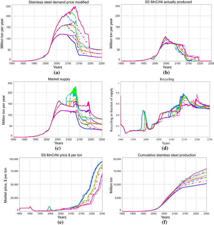

  

  A sensitivity analysis based on nickel resource sizes and demand levels for stainless steel. a Effect on the demand after modification by price the amount MnCrNi stainless steel produced, b effect on the market supply of stainless steel, d the degree of recycling as a fraction of supply, e the market price in $ per ton stainless steel and f the cumulative amount stainless steel produced

  Fig. 19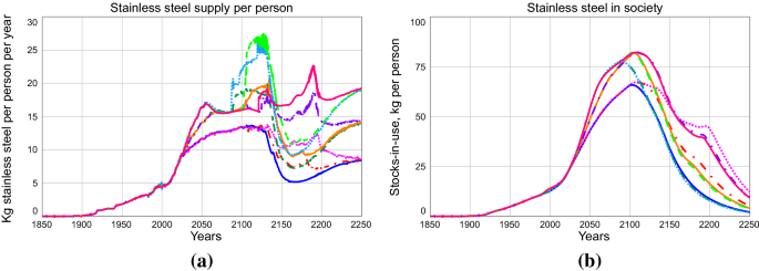

  

  The stainless steel supply in kg per person and per year (a) and the amount stainless steel in use in society as kg per person from the sensitivity simulation (b)

Table 1 shows an overview of important alloying metals for stainless, heat resistant or high hardness steels. Specialty alloys are made using metals like molybdenum, vanadium, niobium, cobalt and tungsten. In this study, we have considered iron, manganese, chromium and nickel. Table 2 shows an overview of important alloying metals for stainless, heat resistant or high hardness steels and the total amounts that are supplied of these. Stocks-in-use for different metals for 2012–2015 are shown in Table 3. Some reports suggest that there is a saturation level for stainless steel. To our knowledge it has not been shown if this is a true saturation level or just a steady state that appears as if it was a saturation limit. Table 4 shows stainless steel types composition for stainless series 200, 300 and 400, using assumed average compositions based on generic industrial compositions (Adapted, based on information from Yang and Ren (2010), Outokompu (2013) and ISSF (2016). Table 5 shows stainless steel types metal composition, specifying the stainless steel types assumed in the model simulations. When stainless steel of the 300 series cannot be made because of nickel shortage, stainless steel of a type like the 200 and 400 series will be produced. The 400 series has about 11%–points more chromium, and 1–3%-points more manganese more than the 200 series. The 300 series has 2.5% points more nickel and half to one-fifth the amount of molybdenum and niobium than the 400 series. Molybdenum and niobium, and sometimes vanadium and cobalt are used to substitute for nickel in low-nickel alloys. They may almost fully substitute for nickel, but have a higher price and are produced in smaller volumes. The 400 series is sensitive to corrosion under certain types of chemically corrosive environments. Table 6 shows stainless steel types production in 2014 using market share, and estimating material use for that production, the data was extracted from ISSF (2016), Outokompu (2013) and information from Yang and Ren (2010).

Table 1 Important stainless steel-associated metals and what they are used for

Table 2 Overview of important alloying metals for stainless steels

Table 3 Stock-in-use for different metals

Table 4 Examples of different stainless style type compositions

Table 5 Stainless steel types metal composition, simplified view, assumed in the model simulations

Table 6 Stainless steel types production in 2014 using market share from ISSF (2015) and internet sources from companies on market shares

The total global carbon steel production was about 1550 million ton per year in 2014, and a unit value of about 300–400 $ per ton, cast iron is about 100 million ton per year, and a unit value of about 400–500 $ per ton. Stainless steel is about 50 million ton per year, and a unit value of about 2500–3400 $ per ton (Fig. 1). The superalloys production is about 25,000 ton per year in 2017, and a unit value of about 20,000–40,000 $ per ton.

Table 7 shows the estimated ultimately recoverable resources (URR), starting from 1900, stratified according to ore grade and mining depth. The data were derived in a separate study, assessing deposits and ore bodies. The resources in brackets are estimated to be present, but have not been built into the model. The metal price stays too low for them to be considered for extraction during the simulation time.

Table 7 Estimated ultimately recoverable resources (URR), starting from 1900, stratified according to ore grade and mining depth

Theory

Modelling

The stainless steel produced in the model simulation is sold as the physical metal in the market, and we ignore the derivatives trade in our economics model. For all the metals, mass balance applies for society:

$$ {\text{Mined}}\,\, + \,\,{\text{Recycled}}\,\, = \,\,{\text{Change in stock{-}in{-}use}}\,\, + \,\,{\text{Recycled}}\,\, + \,\,{\text{Lost irreversibly}} $$

(1)

“Mined” is what we take from the geological reserves, and there is no other net production of new metal into the system. “Change in stock-in-use” is metal kept and being in active use in society and not lost, and “Lost irreversibly” is what is lost in such a way that we cannot retrieve it again, it leaves the system. “Recycled” refers to metals that are circulated in the system. Recycled is present on both sides of the equation, increasing the internal flux, while the external net input may remain low if recycled is large. The more we recycle, the less we need to mine to keep the same amount in society. The term “known” is used for known reserves and “hidden” for resources that are there, but not found yet and “extractable” contains both “Known” and “hidden” resources. Resources are defined as the total amount that can in due time be found and extracted, even if some or much of it would require a higher price and more exploiting effort.

We assume that the present type of society with international trade and general rule of law and order as it is today will persist over the time considered (1850–2350). We assume that a free dynamic market operates for steel, the key alloying metals manganese, chromium, nickel, molybdenum, niobium and for stainless steel throughout the period. This implies that we have a world with global trade and no significant trade barriers. We assume the population and GDP estimated by the WORLD6 model to be adequate to drive demand in the model. The demand is a generic demand from affluency (GDP) and population plus-specific demands from other modules in the WORLD6 model (Fig. 7).

The Model Description

The WORLD6 model attempts to model the world resource supply systems in a way similar to what the World3 model once did (Meadows et al. 1972, 1992, 2005). WORLD6 includes a more complete description of each individual and significant resource (Olafsdottir et al. 2019; Sverdrup and Olafsdottir 2018, 2019a, b; Sverdrup and Ragnarsdottir 2014, 2016a, b; Sverdrup et al. 2013a, b, c, 2014a, b, 2015, 2017a, b, c, d, 2018a, b, c). However, WORLD6 is not World3, nor has any of the original code of World3 inside. On the principal level, the models differ as follows. In World3, all resources were aggregated to one natural resources indicator R. In WORLD6, this is done very differently. Metals, materials and fossil fuels are done separately and communicate through feedback loops and market mechanisms. WORLD6 has a detailed energy model, whereas in World3, energy was lumped with materials inside the natural resources indicator R. WORLD6 has a biophysical feedback economics model, with cash, investments, depreciation, and financing with debts. World3 did not really have any economic model at all, only a money box. When that ran empty in World3, the model predicted a world collapse. WORLD6 has an adaptive biophysical economic model inside, and during times of deficits, financing can be done using loans and price adjustments. In WORLD6 the world does not crash from a cash deficit. Then loans are made and the crisis bridged. During a crisis, growth can become contraction and economic recession. But it takes extreme events to crash the world in WORLD6. The industrial extraction is depending on the capital allocated to resource extraction. Manufacturing of consumer goods are dependent on capital invested in manufacturing sector to keep going. The WORLD6 model has these capital stocks: cash money, extractive Industrial capital, manufacturing Industrial capital, financial capital, society capital, military capital and black capital. It has separate debt stocks, pension obligations, and bank debts. If the Extractive Industrial Capital falls below a certain intensity per produced unit, the production will be reduced. The capital is worn down over time in the model and maintained by investments.

Full technical description of the model is found in Koca et al. (2017), Sverdrup and Koca (2017, 2018), Lorenz et al. 2017 and Hirschnitz-Garbers et al. (2018a, b). Nickel and stainless steel are often recycled because of their value, while chromium and manganese are not. Many specialty purpose metals and materials may face issues of scarcity, but these are minor in importance to the three mentioned above. If society fails on any of those, other shortages are redundant. The WORLD6 model does contain several other modules as well (Sverdrup et al. 2009), but these are outside the scope of this study and will not be further described here. The flow pathways, the causal chains and feedbacks loops in the global iron system were mapped using system analysis, and the resulting coupled differential equations were transferred to computer codes for numerical solutions. The model is based on mass balance expressed differential equations, and solved numerically with a 4-step Runge–Kutta method, using a 1/512-year time-step in the integration. The model was used for quantification of flows, scenarios and future predictions. The model was developed to estimate supply, extractable amounts stocks, price and stocks, and flow in society in the time interval 1900–2400. The model has the following modules used to define the coupled nonlinear differential equations defined by mass balance:

• 1. Source modules in WORLD6

  • a. Metals for alloying and their prices in the model:

    • i. Iron (Koca et al. 2017; Sverdrup and Koca 2017; Sverdrup and Olafsdottir 2019a)

    • ii. Manganese (Sverdrup and Olafsdottir 2019a)

    • iii. Chromium (Sverdrup and Olafsdottir 2019a)

    • iv. Nickel (Sverdrup and Olafsdottir 2019a)

    • v. Molybdenum and Rhenium (Sverdrup and Olafsdottir 2018)

    • vi. Niobium (Sverdrup and Olafsdottir 2018)

  • b. Energy; coal and electricity (Koca et al. 2017, Sverdrup and Koca 2017)

  • c. Population (Koca et al. 2017, Sverdrup and Koca 2017)

  • d. GDP: From the Biophysical economic model (Sverdrup et al. 2018a, b, c; Sverdrup 2019)

• 2. Stainless steel

  • a. Trade market stocks

    • 1. MnCrNi

    • 2. MnCr

    • 3. Dependent variable: Total stainless steel market (MnCrNi + MnCr)

  • b. Stock-in-use

    • i. Material; Slow turnover stocks-in-use

      • 1. MnCrNi

      • 2. MnCr

    • ii. Material: fast turnover stocks-in-use

      • 1. MnCrNi

      • 2. MnCr

  • c. Scrap stock

    • i. Material in scrap

      • 1. MnCrNi

      • 2. MnCr

MnCrNi is the abbreviation for high-quality stainless steel in the model; MnCr is the abbreviation for lower-quality steel with reduced nickel content. All the reserves and resources for the raw materials have been graded into five different ore grades (rich, high, low, ultralow, trace). In addition to the mass balances comes equations for ore grades, energy use and summing up of cumulative amounts of energy use, waste rock and ore grades. The ore was mined from the grade with the lowest extraction cost with some overlap between the ore grade classes. Dependent stocks contain cumulative amounts of: mined materials, rock waste, losses, smelter slag and ore found by prospecting.

Figure 3 shows the flow chart for the model, showing the model for making alloyed steel using iron, manganese, chromium and nickel. The metals flow from reserves, and when they decline, this may limit stainless steel production. In response to stainless steel production demand, supply is made from the manganese, chromium and nickel markets.

The general price model applied to manganese, chromium and nickel, is conceptually the same as that used for aluminium, copper, silver or cobalt. (Sverdrup and Ragnarsdottir 2014, 2016a, b). Less metal in the market causes the price to be higher, decreasing demand, but increasing price causes increasing supply with a delay, when extraction by mining has room to increase. When the market price falls below the mining cost, then the mining extraction is turned off and does not go back on until the price has come up enough to make the mine profitable. For this to happen, the price must be above the mining cost. The price is influenced by the mining cost. The lower the ore grade, the more expensive it gets (Sverdrup and Olafsdottir 2019a; Gutowski et al. 2016). Supply to stainless steel production is controlled by the metal price and profit in 4 different markets: iron, manganese, chromium and nickel. We have kept the alloy formula for the two types of stainless steel constant and when one formula cannot be done, then it is not modified, but we change to another type of stainless steel (Fig. 4). In the simulation, we will use two types of stainless steel:

• 1. MnCrNi type Stainless steel with the average composition as given in Table 7 is used in the model; Fe 61%, Ni 6.4%, Cr 17.8%, Mn 14%, Mo 0.35% and Nb 0.15%

• 2. MnCr type Stainless steel composed without nickel as given in Table 6 is used in the model; Fe 56%, Cr 22%, Mn 20%, Mo 0.75% and Nb 0.5%

Stainless steel has small amounts of carbon, silicon and nitrogen in the alloy. Stainless steel under model type MnCrNi is made first to fulfil the stainless steel demand. When supply cannot keep up with demand after price modification because of shortage of nickel (most of the time), chromium (some limited periods) or manganese (always enough), a model type MnCr is made. The scheme for how this is done is illustrated in Fig. 4. Figure 5 shows the causal loop diagram for the model, for the additions to the causal loop diagram for iron (Sverdrup and Olafsdottir 2019a). Using the WORLD6 model market simulations implies that there is never an equilibrium in the simulated market. That it is the result of the market dynamics between demand and supply (mining and recycling), where price equilibrium may never be reached. A lower ore grade implies that more rock must be moved to mine the iron. The price is set relative to how much iron or steel there is available in the market. The higher the ore grade is, the mining cost will be less and less mining cost leads to more mining profit resulting in more mining putting more mined material to the market. The more material is available for sale on the market, the lower the price gets.These market mechanisms and their parameterization are explained in detail in the paper: Conceptualization and parameterization of the market price mechanism in the WORLD6 model for metals, materials and fossil fuels (Sverdrup and Olafsdottir 2019a). The whole metal cycle has several cores with reinforcing loops as can be seen from the bigger CLD in Fig. 6: an extraction loop driven by resource price and profits, a recycling loop driven by price and profits, a production and resource use loop driven by profits, a consumption loop run by society finances and profits converting to disposable income and consumption that drives demand, and environmental pollution loop that cause more consumption, and a small sustainability loop driven by self-renewal. In the WORLD6 model, gross domestic product (GDP) is the value of all finished goods and services produced per year. In the causal loop diagram, consumption and profits are contributing to the GDP, but not all of it. Note that profits affect the recycling, extraction and production, by the drive for profit and by using the profits for investment and maintenance of the infrastructure.

The extraction of fossil resources is a balancing loop, eventually stopping mining when the resource runs out. The mining activity is mainly profit driven as the main causal factor, but also affected by the demand. The amount in the market sets the price, which has a feedback on supply (higher price gives more mining when the reserves allow this) and demand (higher prices presses down demand). The supply is increased by increasing the mining of ore and smelting it to metal. Figure 7 shows the causal loop diagram for the resource extraction dynamics. In the present version of the model, a fraction of the GDP is used as a proxy for disposable income, remember that when reading Figs. 6 and 7. The causal loop diagram in Fig. 7 develops how investments are needed to keep the production running. The function showing how higher price promotes more recycling is shown in Fig. 8. The technological advances are reflected in a curve shown in Fig. 8. The curve was developed from similar curves developed earlier for copper and silver (Sverdrup et al. 2014a, b, 2018a, b, c).

In the bigger picture, profits contribute to society finances and disposable income and drive demand through consumption. GDP is currently used as a proxy for disposable income in WORLD6, as a fraction. As the model is developed further, GDP will be replaced with disposable income. Demand is driven by GDP, i.e. it is the need per capita scaled up with GDP. Demand is based on needs before any feedbacks from price or scarcity. Consumption demand per capita is a function of GDP as shown in Fig. 6 (Sverdrup and Olafsdottir 2019a). From that we get Eq. (2) for finding the demand:

$$ {\text{Demand }} = {\text{ Consumption demand per capita }}*{\text{ Population of consumers}} $$

(2)

The demand is then modified with market price, adjusting for the fact that higher price will reduce the real demand (Sverdrup and Olafsdottir 2018):

$$ {\text{Price modified demand}} = {\text{ Demand}}*{\text{ f}}\left( {\text{Market price}} \right) $$

(3)

The function f(market price) reduces the demand and higher price (Sverdrup and Olafsdottir 2019a) and is shown in Fig. 8. The mining of manganese, chromium and nickel is all individually driven by operations profits. The manufacture of stainless steel is also driven by operations profits. The income from operations is estimated from supplied amount times the market price. The costs are estimated from production. The costs consist of fixed costs including capital costs and the variable cost depending on production volume, raw material costs such as iron, manganese, chromium, nickel and additional cost for molybdenum, niobium, flux materials and energy in terms of coke, coal and electricity. The energy prices are derived internally in the WORLD6 model. They increase modestly during the simulation period (Fig. 8). In the WORLD6 model, the following procedure is followed in the production of stainless steel. First, MnCrNi steel is produced to satisfy the demand. For this, we check that we have enough manganese, chromium and nickel.

$$ {\text{Produced amount MnCrNi }} = { \hbox{min} }\left( {{\text{demand}}/{\text{X}}_{\text{Mn}} ,{\text{ demand}}/{\text{X}}_{\text{Cr}} ,{\text{ demand}}/{\text{X}}_{\text{Ni}} } \right) $$

(4)

where demand is the initial demand for MnCrNi stainless steel after modification by price. X_Mn, X_Cr, and X_Ni are content of manganese, chromium and nickel in the stainless type produced. We have defined the composition of the MnCrNi type of stainless steel to be as defined in Table 7. Then we check if the demand has been met, or if there is a deficit. In our simulations, it is always nickel that becomes limiting. The demand for alternative stainless steel as a substitute is estimated as (Fig. 10):

$$ {\text{Demand MnCr}}_{{}} = {\text{ demand }} - {\text{ produced amount MnCrNi}} $$

(5)

It is noted that we have adaptive market mechanisms at work, since we have a supply chain with many actors in every step. Then, the market price is set in the system (a system that consists of many suppliers and many buyers) in an arbitration process. The price equation used in this study is the following (Olafsdottir et al. 2019; Sverdrup et al. 2013a, b, 2014a, b, c, 2015, 2017a, b, c, 2018a, b, c; Sverdrup and Ragnarsdottir 2014; Sverdrup 2017; Sverdrup and Olafsdottir 2018, 2019a):

$$ {\text{Market Price}} = {\text{k*}}\left( {\text{market stock}} \right)^{\text{n}} $$

(6)

In the equation, k is a constant, n is an exponent, showing the degree of scaling in the market, and the market stock is the total amount of a tradable good in the market being immediately being traded and available for shipment at an agreed time (LBMA 2018a,b). Values for k and n have been listed for a number of metals in Sverdrup and Olafsdottir (2019a).

Energy data were gathered by the authors from literature and using semi-published corporate information (EuroInox 2014; ICMM 2012; International Steel Forum 2014; Pauliuk et al. 2013a, b; US EPA 2007; Wang et al. 2007, World Steel Association 2012, 2013a, b, 2014a, b, c, d). This was built into the stainless steel module of WORLD6 model, and when there are global energy shortages, these will be able to limit steel production, potentially also the stainless steel production. Population is generated internally in the WORLD6 model (Sverdrup et al. 2014a, b; Sverdrup and Ragnarsdottir 2014) and is used as an input to the model together with the simulated global GDP to estimate the demand, examples of outputs are shown in Fig. 9.

Results from Simulations

The Base Case Simulation

The model makes stainless steel from iron, manganese, chromium and nickel. Nickel is predicted to become a limiting metal for the production of stainless steel, shifting a part of the stainless steel production towards a chromium-based stainless steel. Figure 11a shows the production rate for stainless steel, specifying demand, modified demand and supply of the different qualities. Figure 11b shows the simulated production as compared to the data (r² = 0.98). Figure 12a shows the simulated production and observed data. Figure 12b shows the global stock-in-society, the stock for MnCrNi type stainless steel of slow turn-over stock in society (50 years), for MnCrNi type stainless steel the fast turnover stock in society (3 years) and for MnCrNi type stainless steel the scrap stock.

The figure shows that the MnCr type stainless steel the fast turnover stock in society (3 years) and MnCr type stainless steel the scrap stock. For MnCr type of stainless steel, we have assumed that it only goes into a fast stock. Figure 12 shows the simulated price and the comparison to the observed data. We have used reconstructed data from the nickel, chromium, manganese and iron price. The price was composed from the price of iron (71%), price of manganese (12%), price of chromium (11%) and price of nickel (8%), and we multiplied the result with a factor of 1.7 for other costs.

According to the literature (UNEP reports), the stainless steel recycling rate was estimated at approximately 25% in 2015, which is matched by the model simulation. We have shown two types of price, one is the simulated price for MnCrNi stainless steel, and the other is a price simulated for all stainless steel in the market. The market price level and long-term trends are reasonably well captured by the model, but many of the short-term variations are not (Fig. 13). The main reason for this is that many aspects of short-term trading (hedging, derivatives, forwards) are not included in the model. The details of such transactions have poor transparency, and it is a major challenge to model and parameterize them based on mass balance and market mechanism observations. Figure 14a shows the stainless steel supply per person per year is the provision for maintenance, losses and growth in stainless steel. The stock-in-use per person is an indicator of the level of service provision by stainless steel. The implication is that growth in the stainless steel industry is over in terms of volume by 2050. The monetary value will continue to increase, as the price will go up at the same time. Figure 14b shows the stainless steel recycling as a fraction of the total stainless steel supply and Factor X for stainless steel. Factor X is the cumulative total supply over the cumulative amount produced of stainless steel. It expresses how many times a ton of stainless steel is used before it is lost. Figure 15 shows the cumulative amount of stainless steel produced as compared to the observed cumulative amount for stainless steel and the simulated stainless steel production rate as compared to the available data to 2017. The graphs test the long-term consistency of the model, which appears to be very good (see also in Fig. 16).

Testing the Predictions

The model outputs were checked against the observed data. In Fig. 15a, plot for the stainless steel production rate is presented, the simulation fits well to the data with r² = 0.97. Figure 15b shows the simulation output for the cumulative amounts supplied, using the data from Fig. 11a, for the time period 1850–2017, tested against the observed data. The simulation production rate output fits well with the observed data, with a correlation coefficient of r² = 0.998.

Sensitivity Analysis

Variations in Stainless Steel Demand and Nickel Resource Size

A sensitivity analysis was performed based on many runs with the model and many different scenarios tested. We show the effect of varying nickel extractable resource sizes (URR) and different levels of stainless steel demand after 2020. All runs have the same demand as in the business-as-usual scenario. For stainless steel, it appears that the limiting factor is nickel availability, and any potential manganese, chromium and iron shortages are redundant to that. The variations used were:

• The stainless steel demand was set at three different levels, starting in 2020, but multiplying with a factor to scale it up or down. The demand curves resulting from this are shown in Fig. 17b. The stainless steel demand translates internally in the WORLD6 model to partial demands for manganese, chromium, nickel and iron, as well as the specialty metals niobium and molybdenum. These demand all translate to energy demands in the WORLD6 model that eventually increases the production costs.

• The nickel resource was set at three different levels, 800 million ton, 700 million ton and 600 million ton. The result of this is shown in Fig. 17a.

To untangle the effect of nickel resource, look at the outputs before 2030, most of that variation is due to difference in resource size. After 2050, the effect of demand variation is more pronounced. The upper line is the line for the largest nickel resource, and then, it can be seen how that fans out as different demands kick in. The middle line before 2020 is the middle resource; this also fans out caused by different demands after 2030. The lowest line is the lowest resource; this fans out because of the different demands coming in after 2020. For the demand after price modification (Fig. 18a), both resource variation and demand based on need variation have an effect on the demand after price feedback. But in terms of stainless steel actually produced, there is less freedom for variation which is seen in Fig. 18b. That small variation, plus the caused variation in recycling (Fig. 18d), which is driven by price increases (Fig. 18e), results in variations in actual supply to the market. Most of that variation is driven by the variation in the demand (Fig. 18c). To understand the diagrams, we need to have the causal loop diagrams for the subsystem in our minds (Fig. 19).

Other variations were tried, but most of these gave little change in the general trends, and are not worth showing. The reasons for this are twofold. Some of the variations are overruled by other variations (Nickel limitations occur before chromium limitations, thus varying chromium demand or resource did not give and difference. And some parameters varied were simply not very important. Because of all the feedbacks in the system, especially through the economic modules, the system is compensating for some of the variations made. Thus, a sensitivity analysis using only parameter variations will only test a part of the sensitivity. It was considered to be beyond the scope of these study to investigate the sensitivity of the results with respect to the feedback structure of the integrated WORLD6 model system. Figure 20 shows the model outputs using nickel resource variations and stainless steel demand variations used in the sensitivity analysis corresponding to sensitivity simulation. We show the following: the demand after modification by price, the amount MnCrNi stainless steel produced, the market supply of stainless steel, the amount stainless steel recycled to stainless steel, the degree of recycling as a fraction of supply, the market price in $ per ton stainless steel. The diagrams in Fig. 18 show the model sensitivity run output for the amount stainless steel in use in society as kg per person (Fig. 20a) and stocks in use per person (Fig. 20b). The stainless steel supply to society in kg stainless steel per person per year is showing the provision of service from stainless steel per person. This is an indicator for utility in society. Increasing the stainless steel demand makes the stainless steel production rate at the peak higher, and the time of the stainless steel production maximum comes earlier. The stainless steel stocks in use will reach a higher level with increased demand. Increasing the nickel resource make the stainless steel production rate decline come later, and the decline in stainless steel stocks in use come later. Increasing the extractable resource extends the supply curve in time.

Fig. 20

This figure is using the WORLD6 model to explore one possibility on what could happen in the very long term based on simulation outputs for: a the amount of stainless steel in use in society as kg per person, b the stainless steel supply in kg per person and per year, c the amount in use in society as kg per person for nickel, manganese and chromium and d the supply in kg per person and per year for nickel, manganese and chromium

Looking at Different Time Horizons

We have allowed ourselves to ask a “what if” question. One such question would be to ask “Could even metals like iron, or manganese or chromium run out if we looked far enough into the future?” Using the WORLD6 model like that, does not in any way propose that this will actually happen. But it explores what would be possible, suggesting that it could happen if all our assumptions are valid for the whole period. For this purpose, we ran the WORLD6 model for 1800 years into the future, to 3800 AD, just to see what would happen in the very long run, assuming business-as-usual would just go on, with the feedback we have today. This is shown in Fig. 21. It turns out that a critical time occurs around 2500 AD. Then most metals resources will have been depleted. Iron will be in abundant supply per person until about 2450, but then a sharp decline sets in. The same happens to manganese and chromium, then are sufficient until about 2500, and then the final decline comes, whereas the supply of nickel will be a trickle after 2300. If a transition to photovoltaic energy, wind energy and thorium-based nuclear power can be successfully made, the energy availability will be sufficient to 3600 AD and beyond. The stocks in society will pass below those we have at present between 2500 and 2700 AD. That would be about 700 years from now, or less than 20 generations, well within many existing family trees if were to go backward in time. Figure 20a shows the amount stainless steel in use in society as kg per person indicating a rapid decline from 2260, and Fig. 20b shows the stainless steel supply in kg per person and per year. For stainless steel, the trend is declining from 2100 even though we see four minor spikes in the downward slope. Figure 20c shows the amount in use in society as kg per person for nickel, manganese and chromium, indicating that amounts of nickel and manganese per person will peak around 2100 peak and then decline rapidly. For nickel, the amount runs close to zero around 2350. Figure 20d shows the supply in kg per person and per year for nickel, manganese and chromium. It can be seen that nickel is the element where the supply declines to near zero first (around 2300) (Fig. 22).

Fig. 21

In the diagram showing the plot from Fig. 11a, we have explained the difference between soft scarcity and hard scarcity that can be seen to be predicted for stainless steel. The diagram shows when scarcity occurs, substitution by a lower quality type of stainless steel occurs for some of the shortage. “D modified” is demand after price,modification. “All recycled” implies both directly recycled and recycled as part of an alloy

Fig. 22

a Development of the ore grades over time for manganese, chromium, iron and nickel as simulated by the model (b)

Discussion

The Importance of the Nickel Resources Available

It appears that nickel is the key limiting composition element for the stainless steel production. Supply of nickel reaches a maximum in 2050, an indication that that is also the maximum supply year for stainless steel (Fig. 21). The next metal that could become limiting for stainless steel would be chromium, but that never occurs in any of the runs, nickel limits the production first. Manganese seems to always be sufficient for all alternatives. When the ore grade declines, the extraction costs rise significantly and the price goes up (see Fig. 23d). That in combination with demand that exceeds the supply, driving the stainless steel price up by both pushing and pulling. The expression of resource exhaustion has two aspects that must be considered. The first is the amount of extractable resource, not yet extracted, that will go down over time. It is beyond any doubt that these fossil resources, those that are not yet extracted, are declining. At the same time, the quality of the resource is also declining, as common practice is to extract the best quality first (this is seen from Fig. 23). That goes a long way to explain the gradual increase in price. The price mechanism acts in such a way that supply and demand drive the price down or up, but if the price falls below the extraction cost, supply simply stops until the price has come back up above the break-even point. The evolution of the metal prices during 1950–2250 has been shown in Fig. 23d. In the simulations, chromium was the next metal to become limiting, later molybdenum and niobium became limiting for the MnCr type of stainless steel. A residual of manganese was left. Small amounts of molybdenum and niobium are added to both types of stainless steel. MnCr steel requires more molybdenum and niobium to compensate for the lack of nickel. It resembles a Martensitic type of stainless steel with no nickel. The activity in the model is driven by the condition that the operations must run with a profit. Figure 23a shows and overview of the approximate profitability of the steel sector according to the simulations and the approximate profit calculated for each metal and for stainless steel. The costs of extraction have been plotted in and for comparison; the global GDP was put in the same curve. These show the aspect that extraction costs rise sharply when the ore grade declines. But it is also important to realize that the dynamics of the steel production sector is only partly explained by the individual variables, and to a larger degree by the actual dynamics defined by the system structure itself through causal links and feedback structures. During the simulation period, the energy price increases some. But the amount used increases more as the ore grades decline, and the increase in total energy use per unit, combined with larger amounts, makes the energy volumes used for steel and stainless steel very significant.

Fig. 23

Overview of the approximate profitability of the steel sector according to the simulations (a) and the approximate profit calculated for each metal and for stainless steel (b). The costs of extraction have been plotted in (c) and for comparison, the global GDP was put in the same curve. SS stainless steel. d Market price for manganese, chromium, iron and nickel as simulated by the model in $ per ton

Substitution

Assuming the GDP growth profiles and mining costs in the model are accurate for the future, the results imply that nickel production will start to decline in 2050, after peaking at about 68 million to per year (Sverdrup et al. 2018a, b, c). The missing amount of MnCrNi type of stainless steel can be replaced by a simpler chromium–manganese stainless steel alloy, enhanced with more molybdenum and niobium. The total supply of molybdenum is 310,000 ton per year (2018), vanadium is 89,000 ton per year (2018) niobium is 85,000 ton per year (2018) or cobalt is 90,000 ton per year (2018); they are all far too small to act as proper volume substitutes for nickel (2,300,000 ton per year in 2018), even if less content is used in new types of stainless steels (Table 2). The sum of the production rates for molybdenum, vanadium, niobium and cobalt is about 465,000 ton per year. Substitution of stainless steel for alloys based on these metals is only possible on a small scale. The stock-in-use of stainless steel in society will reach a maximum in 2085 and then slowly decline. In Fig. 16, we have explained the difference between soft scarcity and hard scarcity that can be seen to be predicted for stainless steel. Soft scarcity from 2150, and hard scarcity from 2180. Substitution of high-grade stainless steel with low grade takes stainless steel place from 2140. The development of the ore grades over time for manganese, chromium, iron and nickel is shown in Fig. 18. The market price for manganese, chromium, iron and nickel all rise during the period. The increase in nickel price and energy price is the main reason why the price goes up for stainless steel. The prices for manganese and chromium will be increasing, but they are not at high prices to begin with and contribute less to the price of stainless steel.

Conclusions

The WORLD6 model was used, and it shows that finite resources peak and decline even with recycling and the full compensating effect of a dynamic economy included. The conclusion would seem to be that, given the set of assumptions about recycling rates, costs and the data used, that if stainless steel production growth continues, planners and policy-makers could expect to see a crunch in supply that could arrest growth within the next 30 years for conventional stainless steels. This is not new in qualitative terms (Bardi 2013; Sverdrup and Ragnarsdottir 2014), but this time the care was taken to include all the dynamics, and the qualitative conclusion is now quantitatively shown. For stainless steel production, we may make the following conclusions:

• 1. Nickel seems to be the critical metal for stainless steel production. After 2050, nickel supply will decline, and by 2090, the production of Mn–Cr-based stainless steel will be more than the produced amount of Mn–Cr–Ni stainless steel. This is a physical limitation on the source of primary extracted nickel and can only be mitigated by more recycling. There will be challenges with declining ore grades and rising extraction costs in the next 50 years, driving nickel prices up.

• 2. The first sign of stainless steel scarcity is not through physical limitation, but rather through increases in stainless steel prices, which in turn affect both supply and the demand of stainless steel (Fig. 21).

• 3. Chromium and manganese seem to be sufficiently abundant and will not run into any significant scarcity before 2300. There may be challenges with declining ore grades and rising extraction costs in the next 50 years, driving chromium prices up.

• 4. Niobium, molybdenum, vanadium and cobalt cannot substitute significantly for nickel in stainless steel in large amounts (Sverdrup and Olafsdottir 2018; Sverdrup et al. 2018a). Nickel has an annual primary production of more than 2.5 million ton per year, whereas niobium, molybdenum, vanadium and cobalt are produced in smaller amounts.

For global sustainability, we have the following conclusions from this study: running out of iron, steel and stainless steel on large global scale will make many other big issues we are facing globally appear as small problems. The turn-over of steel and stainless steel and the commodity production based on these materials is a significant part of the whole global economy. A decline in steel and stainless steel supply will create a decline the global economy.

Mn–Cr stainless steel alloys will have to take some of the place of Mn–Cr–Ni stainless steel alloys in the future, but the reserves and production rates of metals like cobalt, molybdenum, tantalum or vanadium are far small to be viable substitutes for nickel in the alloys. These metals are limiting on their own as important ingredients for super-alloys and specialty steels. With increased price because of scarcity, we may expect recycling to go up and soften the decline somewhat. At recycling degrees above 80%, the supply of nickel, chromium and manganese will be sufficient for several centuries.

Discussion

Unless global population growth can be managed and brought to a net population decrease by 2100, iron, steel and stainless steel scarcity will be a reality. An alternative is that the total metal use is reduced and the circularity of metal handling changes in some fundamental way. Even though this paper did not cover the social implications that such scarcity might lead to, it is likely to be huge. Other aspects also not covered in this paper but worthy of thought in this relation are the energy limitations that are likely to become a large issue with iron and steel production by 2100. The tests show that the model can simulate the observed production rates for stainless steel. The metal prices are generated endogenously based on price dynamic feedbacks that have been captured in the WORLD6 model. The model seems to perform well when tested against field data for production rates over time.

References

Alonso E, Frankfield JG, Kirchain R (2007) Material availability and the supply chain: risks, effects, and responses. Environ Sci Technol 41:6649–6656
Bardi U (2013) Extracted. How the quest for mineral wealth is plundering the planet. The past, present and future of global mineral depletion. A report to the Club of Rome. Chelsa Green Publishing, Vermont
Bellevrat E, Menanteau P (2008) Introducing carbon constraint in the steel sector: ULCOS scenarios and economic modeling. Proceedings of the 4th Ulcos seminar, 1–2 October. www.ulcos.org/en/docs/…/Ref01%20-%20SP9_Bellevrat_Essen.pdf
Brewster N (2009) Outlook for commodity markets. Rio Tinto Inc. MF Global Seminar 2009, ppt slides
Chen WQ, Graedel TE (2012) Anthropogenic cycles of the elements: a critical review. Environ Sci Technol 46:8574–8586
Cobb HM (2010) History of stainless steel. ASM International, Materials Park, OH
Cullen JM, Allwood JM, Bambach MD (2012) Mapping the global flow of steel: from steelmaking to end-use goods. Environ Sci Technol 46:13048–13055. https://doi.org/10.1021/es302433p
Cutler P, Coates G (2012) Stainless steel and nickel, 100 years of working together. Blog. ASSADA. Stainless Steel Focus 7/2012. Australian Stainless Magazine, Issue 52. 3 p. http://www.assda.asn.au/blog/255-stainless-steel-and-nickel-100-years-of-working-together
Daigo I, Matsuno Y, Adachi Y (2010) Substance flow analysis of chromium and nickel in the material flow of stainless steel in Japan. Resour Conserv Recycl 54:851–863
de Beer J, Worrell E, Blok K (1998) Future technologies for energy-efficient iron and steel making. Annu Rev Energy Environ 23:123–205. https://doi.org/10.1146/annurev.energy.23.1.123
Eliott M (2013) Aluminium for steel; aluminium, plastics fiber-optics or steel and graphene for copper; palladium for platinum; iron for nickel; potential rare earths substitution. In: Supercycle hangover; The rising threat of substitution. pp 8–10
Eliott M et al (2014) Business risks facing mining and metals 2014–2015. EY Report 56 pp. http://www.ey.com/GL/en/Industries/Mining-Metals/Business-risks-in-mining-and-metals
EuroInox (2014) International Stainless Steel Forum Austenitic chromium-manganese stainless steels, A European approach. The European Stainless steel development Association. Materials and application Series. EuroInox, Pavia, pp 2–20
Forrester J (1971) World dynamics. Pegasus Communications, Waltham MA
Giurco D, Cohen B, Langham E, Warnken M (2012) Backcasting energy futures using industrial ecology. Technol Forcasting Soc Change 78:797–818
Graedel TE, Erdmann L (2012) Will metal scarcity impede industrial use? Metals Res Soc Bull 37:325–333
Graedel TE, Buckert M, Reck BK (2011) Assessing mineral resources in society. Metal stocks and recycling rates. UNEP, Paris
Graedel TE, Harper EM, Nassar NT, Reck B (2015a) On the materials basis of modern society. Proc Natl Acad Sci USA 112:6295–6300. https://doi.org/10.1073/pnas.1312752110
Graedel TE, Harper EM, Nassar NT, Nuss P, Reck B (2015b) Criticality of metals and metalloids. Proc Natl Acad Sci USA 112:4257–4262. https://doi.org/10.1073/pnas.1500415112
Guirco D, Littleboy A, Boyle T, Fyfe J, White S (2014) Circular economy: questions for responsible minerals, additive manufacturing and recycling of metals. Resources 3:432–453. https://doi.org/10.3390/resources3020432
Gutowski TG, Sahni S, Allwood M, Ashby MF, Worrell E (2016) The energy required to produce materials: constraints on energy-intensity improvements, parameters of demand. Philos Trans R Soc A 371:20120003. https://doi.org/10.1098/rsta.2012.0003
Hall C, Lindenberger D, Kummel R, Kroeger T, Eichhorn W (2001) The need to reintegrate the natural sciences with economics. Bioscience 51:663–667
Haraldsson HV, Sverdrup HU (2004) Finding simplicity in complexity in biogeochemical modelling. In: Wainwright J, Mulligan M (eds) Environmental modelling: a practical approach. Wiley, Chichester, pp 211–223
Haraldsson HV, Belyazid S, Sverdrup H (2006) Causal loop diagrams, promoting deep learning of complex systems in engineering education. In: Alveteg M, Leire E (eds) LTH pedagogiske inspirasjonskonferens. pp 1–4
Hasanbeigi A, Morrow W, Sathaye J, Masanet E, Xu T (2012) Assessment of Energy Efficiency Improvement and CO2 Emission Reduction Potentials in the Iron and steel Industry in China. Report. Berkeley, CA: Lawrence Berkeley National Laboratory Report LBNL- LBNL-5535E
Hasanbeigi A, Price L, Arens M (2013) Emerging energy-efficiency and carbon dioxide emissions-reduction technologies for the iron and steel industry. Ernest Orlando Lawrence Berkeley National Laboratory. LBNL-6106E
Hatayama H, Daigo I, Matsuno Y, Adachi Y (2010) Outlook of the world steel cycle based on the stock and flow dynamics. Environ Sci Technol 44:6457–6463
Heinberg R (2011) The end of growth. Adapting to our new economic reality. New Society Publishers, Gabriola Island
Hirschnitz-Garbers M, Koca D, Sverdrup H, Meyer M, Distelkamp M (2018) System analysis for environmental policy—System thinking through system dynamic modelling and policy mixing as used in the SimRess project Models, potential and long-term scenarios for resource efficiency (SimRess) Texte 50-2018. 281 p. FKZ 3712 93 102, Verlag Umweltbundesamt. Berlin. https://www.umweltbundesamt.de/publikationen/system-analysis-for-environmental-policy-system-0
Hirschnitz-Garbers M, Distelkamp M, Koca D, Meyer M, Sverdrup H (2018) Potentiale und Kernergebnisse der Simulationen von Ressourcenschonung(spolitik) Endbericht des Projekts „Modelle, Potentiale und Langfristszenarien für Ressourceneffizienz“(Sim-Ress) Texte 48-2018. 86 pages. FKZ 3712 93 102, Verlag Umweltbundesamt. Berlin. https://www.umweltbundesamt.de/publikationen/potentiale-kernergebnisse-der-simulationen-von
Hsu F-C, Eidvige CD, Matsuno Y (2011) Estimating in-use steel stock of civil engineering and building in China by nighttime light image. Proc Asia-Pacific Adv Netw 31:58–68. https://doi.org/10.7125/APAN.31.7ISSN2227-3026
Hu M, Pauliuk S, Wang T, Huppes G, Voet E, Müller D (2010) Iron and steel in Chinese residential buildings; A dynamic analysis. Resour Conserv Recycling 54:591–600
International Stainless Steel Forum (2014) The stainless steel family. 5 pp International Stainless Steel Forum Rue Colonel Bourg 120 B-1140 Brussels Belgium, www.worldstainless.org
International Stainless Steel Forum (2016) The stainless steel in figures 2016. 51 pp. International Stainless Steel Forum. Rue Colonel Bourg 120 B-1140 Brussels Belgium, www.worldstainless.org
International Trade Administration (2016) Global Steel Trade Monitor. Global Steel Report. 15 p
Kalenga M, Xiaowei P, Tangstad M (2013) Manganese alloys production: Impact of chemical compositions of raw materials on the energy and materials balance. Manganese Fundamentals. Proceedings of the thirteenth International Ferroalloys Congress on efficient technologies in ferroalloy industry June 9–13, 2013 Almaty, Kazakhstan. pp 647–675
Kennedy P (1987) The rise and fall of the great powers: Economic change and military conflict from 1500 to 2000. Random House, New York
Koca D, Sverdrup H, Ragnararsdottir V (2017) Kausalschleifendiagramme als narrative Visualisierungs- Tools für Kommunikation und Analyse komplexer dynamischer Systeme: Konzeptuelle Modellierung und Systemanalyse von komplexen Mensch-/Natur-Systeminteraktionen in einer Welt mit begrenzten Ressourcen als Beispiel. In: Biemann, K, Distelkamop, M., Dittrich, M., Dünnbell, Greiner, B., Hirschnitz-Garber, M., Koca, D., Sverdrup, H., Kosow, H., Lorenz, U., Mellwig, P., Meyer, M., Neumann, K., Schoer, K., van Oechsen, A., Weimer-Jehle, W., (Eds). Sicherung der Konsistenz und Harmonisierung von Annahmen bei der kombinierten Modellierung von Ressourceninanspruchnahme und Treibhausgasemissionen. Reader zum Erfahrungsaustausch im Rahmen des SimRess-Modellierer-Workshops am 7-8 Dezember in Berlin. Simulation Ressourceninanspruchnahme und Ressourceneffizienzpolitik pp 37–45. DOKUMENTATIONEN 04/2017 Umweltforschungsplan des Bundesministeriums für Umwelt, Naturschutz, Bau und Reaktorsicherheit. Forschungskennzahl 3712 93 102 ISSN 2199-6571 Dessau-Roßlau, Januar 2017
Lorenz U, Sverdrup HU, Ragnarsdottir KV (2017) Global megatrends and resource us—a systemic reflection. In: Hinzmann M, Evans N, Kafyke T, Bell S, Hirschnitz-Garbers Martina Eick (eds) Factor X; Challenges, implementation strategies and examples for a sustainable use of natural resources. Springer, New York, pp 31–44
Mason L, Prior T, Muss G, Giurco D (2011) Availability, addiction and alternatives: three criteria for assessing the impact of peak minerals on society. J Cleaner Prod 19:958–966
McGarvey B, Hannon B (2004) Dynamic modelling for business management. Springer, New York
Meadows DH, Meadows DL, Randers J, Behrens W (1972) Limits to growth. Universe Books, New York
Meadows DL, Behrens WW III, Meadows DH, Naill RF, Randers J, Zahn EKO (1974) Dynamics of Growth in a Finite World. Wright-Allen Press Inc, Massachusetts
Meadows DH, Meadows DL, Randers J (1992) Beyond the limits: confronting global collapse, envisioning a sustainable future. Chelsea Green Publishing Company, White River Junction
Meadows DH, Randers J, Meadows D (2005) Limits to growth. The 30 year update. Universe Press, New York
Milford RL, Pauliuk S, Allwood JM, Müller DB (2013) The roles of energy and materials efficiency in meeting steel industry CO2 targets. Environ Sci Technol 47:3455–3462
Modaresi R, Pauliuk S, Løvik AN, Müller DB (2014) Global carbon benefits on material substitution in passenger cars until 2050 and the impact on the steel and aluminium industries. Environ Sci Technol 48:10776–10784
Morfeldt J, Nijs W, Silveira S (2015) The impact of climate targets on future steel production e an analysis based on a global energy system model. J Cleaner Prod 103:469–482
Moynihan M, Allwood JM (2012) The flow of steel into the construction sector. Resour Conserv Recycl 68:88–95
Mudd GM, Jowitt SM (2014) A detailed assessment of global nickel resource trends and endowments. Econ Geol 109:1813–1841. https://doi.org/10.2113/econgeo.109.7.1813
Mudd GM, Weng Z, Jowitt SM, Turnbull ID, Graedel TE (2013) Quantifying the recoverable resources of by-product metals: the case of cobalt. Ore Geol Rev 55:87–98
Müller DB, Wang T, Duval B, Graedel TE (2006) Exploring the engine of anthropogenic iron cycles. Proc Natl Acad Sci 103:16111–16116. https://doi.org/10.1073/pnas.0603375103
Norgate TE, Rankin WJ (2002) The role of metals in sustainable development. Proceedings, green processing 2002, international conference on the sustainable processing of minerals, May 2002, pp 49–55
Nuss P, Eckelmann MJ (2014) Life Cycle Assessment of Metals: a Scientific Synthesis. PLoS ONE 9:e101298. https://doi.org/10.1371/journal.pone.0101298
Nuss P, Harper EM, Nassar NT, Reck BK, Graedel TE (2014) Criticality of Iron and its principal alloying elements. Environ Sci Technol 48:4171–4177. https://doi.org/10.1021/es405044w
Olafsdottir AH, Sverdrup H, Ragnarsdottir KV (2019) On the metal contents of ocean floor nodules, crusts and massive sulphides and a preliminary assessment of the extractable amounts. In: Ludwig Chr, Valdivia S (eds) Progress towards the resource revolution, highlighting the importance of the sustainable development goals and the Paris climate agreement as calls for action. World Resources Forum, Villigen PSI and St. Gallen, Switzerland, pp 150–156
Outokompu (2013) Handbook of Steel. 92 pages. Outokompu, Sandviken, Sweden
Papp JF (1994) Chromium life cycle study. II Series. Information circular. United States Buerau of Mines. 9411. HD9539.CAP 1994 338.2’74643-dc20 94-29994 CIP. 100 pp
Pauliuk S, Wang T, Müller D (2012) Moving towards the circular society, the role of stocks in the Chinese steel cycle. Environ Sci Technol 46:148–151
Pauliuk S, Wang T, Müller DB (2013a) Steel all over the world: estimating in-use stocks of iron from 200 countries. Resour Conserv Recycl 71:22–30
Pauliuk S, Milford RL, Müller DB, Allwood JM (2013b) The steel scrap age. Environ Sci Technol 47:3448–3454
Pauliuk S, Wood R, Hertwich EG (2015) Dynamic models of fixed capital stocks and their application in industrial ecology. J Ind Ecol 19:104–116
Plunkert PA, Jones TS (1998) Metal prices in the United States through 1998. USGS, Washington DC, p 184
Prior T, Giurco D, Muss G, Mason L, Behrish J (2012) Resource depletion, peak minerals and the implication for sustainable resource management. Global environmental change. 22:577–587
Prior T, Daly J, Mason L, Giurco D (2013) Resourcing the future: using foresight in resource governance. Geoforum 44:316–328
Ragnarsdottir KV, Sverdrup H, Koca D (2011) Assessing long-term sustainability of global supply of natural resources and materials. 5;83–116. In; Sustainable Development – 116. Energy, Engineering and Technologies – Manufacturing and Environment. Ghenai, C. (Ed.). www.intechweb.org
Ragnarsdottir KV, Sverdrup H, Koca D (2017) Substitution of metals in times of potential supply limitations: What are the mitigation options and limitations? Proceedings of the 2015 World Resources Forum, 11–15 Sept. Davos, Switzerland. In: Ludwig C, Matasci C (eds) Boosting resource productivity by adopting the circular economy. Paul Scherrer Institute, Villingen, Switzerland. pp 84–89. ISBN 978-3-9521409-7-0
Reck B, Graedel TE (2012) Challenges in Metal Recycling. Science 337(690):7
Roberts N, Andersen DF, Deal RM, Shaffer WA (1982) Introduction to computer simulation: a system dynamics approach. Productivity Press, Chicago
Rosenqvist T (1983) Principles of extractive metallurgy. McGraw-Hill Book Company, New Delhi
Senge P (1990) The fifth discipline. The art and practice of the learning organisation. Century Business, New York
Senge PM, Smith B, Schley S, Laur J, Kruschwitz N (2008) The necessary revolution: how individuals and organisations are working together to create a sustainable world. Doubleday Currency, London
Seppelt R, Manceur AM, Liu J, Fenichel EP, Klotz S (2014) Synchronized peak-rate years of global resources use. Ecol Soc 19:50–64. https://doi.org/10.5751/ES-07039-190450
Smith VL (2009) Economics of production from natural resources. Energies 2:661
Sterman JD (2000) Business dynamics, system thinking and modelling for a complex world. Irwin McGraw-Hill, New York
Stockwell LE (1999) World mineral statistics 1993–97: production, exports, imports. British Geological Survey, Keyworth
Sverdrup H (2017) Modelling global extraction, supply, price and depletion of the extractable geological resources with the LITHIUM model. Resour Conserv Recycl 114:112–129
Sverdrup HU (2019) The global sustainability challenges in the future: the energy and materials supply, pollution, climate change and inequality nexus. In: Holden E, Meadowcraft J, Langhelle O, Banister D, Linnerud K (eds) Our common future, what next for sustainable development? 30 years after the Brundtland report, chap 4. Springer Verlag, Frankfurt, pp 49–75
Sverdrup HU, und Koca D (2017) Der Einsatz des WORLD-Modells im SimRess-Projekt: Sys- temgrenzen, Modell-Interaktion, Indikatoren und grundsätzliche Ergebnisse. In: Biemann K, Distelkamop M, Dittrich M, Greiner B, Hirschnitz-Garber M, Koca D, Sverdrup H, Kosow H, Lorenz U, Mellwig P, Meyer M, Neumann K, Schoer K, van Oechsen A, Weimer-Jehle W, (eds) Sicherung der Konsistenz und Harmonisierung von Annahmen bei der kombinierten Modellierung von Ressourceninanspruchnahme und Treibhausgasemissionen. Reader zum Erfahrungsaustausch im Rahmen des SimRess-Modellierer-Workshops am 7–8 Dezember in Berlin – Simulation Ressourceninanspruchnahme und Ressourceneffizienzpolitik. pp 49–71 DOKUMENTATIONEN 04/2017 Umweltforschungsplan des Bundesministeriums für Umwelt, Naturschutz, Bau und Reaktorsicherheit. Forschungskennzahl 3712 93 102 ISSN 2199-6571 Dessau-Roßlau,
Sverdrup H, Koca D (2018) The WORLD Model Development and The Integrated Assessment of the Global Natural Resources Supply. 445 p. Texte 100-2018. FKZ 3712 93 102, Verlag Umweltbundesamt. Berlin. https://www.umweltbundesamt.de/publikationen/the-world-model-development-the-integrated
Sverdrup H, Olafsdottir AH (2018) A system dynamics model assessment of the supply of niobium and tantalum using the WORLD6 model. Biophys Econ Resour Qual 4:1–42
Sverdrup H, Olafsdottir AH (2019a) Conceptualization and parameterization of the market price mechanism in the WORLD6 model for metals, materials and fossil fuels. Mineral Econ. https://doi.org/10.1007/s13563-019-00182-7
Sverdrup H, Olafsdottir AH (2019b) System dynamics modelling of mining, supply, recycling, stocks-in-use and market price for manganese, chromium, nickel and iron. Biophys Econ Resour Qual
Sverdrup H, Olafsdottir AH, Ragnarsdottir KV, Koca D, Lorenz U (2019) The WORLD6 integrated system dynamics model: examples of results from simulations. In: Ludwig Chr, Valdivia S, (eds) Progress towards the resource revolution, highlighting the importance of the sustainable development goals and the Paris climate agreement as calls for action. World Resources Forum, Villigen PSI and St. Gallen, Switzerland, pp 68–76
Sverdrup HU, Ragnarsdottir KV (2014) Natural resources in a planetary perspective. Geochem Perspect 2:1–156
Sverdrup H, Ragnarsdottir KV (2016a) The future of platinum group metal supply; an integrated dynamic modelling for platinum group metal supply, reserves, stocks-in-use, market price and sustainability. Resour Conserv Recycl 114:130–152
Sverdrup H, Ragnarsdottir KV (2016b) Modelling the global primary extraction, supply, price and depletion of the extractable geological resources using the COBALT model. Biophys Econ Resour Qual. https://doi.org/10.1007/s41247-017-0017-0
Sverdrup H, Ragnarsdottir KV (2017) Modelling the global primary extraction, supply, price and depletion of the extractable geological resources using the COBALT model Proceedings of the 2015 World Resources Forum, 11-15 September. Davos, Switzerland. In: Ludwig C, Matasci C (eds) Boosting resource productivity by adopting the circular economy. pp 90–99. Paul Scherrer Institute, Villingen, Switzerland. ISBN 978-3-9521409-7-0
Sverdrup H, Svensson M (2002) Defining sustainability. In: Sverdrup H, Stjernquist I (eds) Developing principles for sustainable forestry, Results from a research program in southern Sweden. Managing forest ecosystems. Kluwer Academic Publishers, Amsterdam, pp 21–32
Sverdrup H, Svensson M (2004) Defining the concept of sustainability, a matter of systems analysis. In: Olsson M, Sjöstedt G (eds) Revealing complex structures—challenges for Swedish systems analysis. Kluwer Academic Publishers, Amsterdam, pp 122–142
Sverdrup H, Koca D, Jönsson-Belyazid U, Belyazid S, Wickberg PO, Haraldsson H, Schlyter P, Stjernquist I (2009) Miljömål i fjällandskapet, en syntes av problemställningar forbundet med förvaltningen av en begränsad ressurs. Peer reviewed with 70 stakeholders during 7 workshops and by scientists at a workshop at Östersund, and by stakeholders at an official public hearing in March 2010 at the Swedish Academy of Sciences, Stockholm, 166 pp. Naturvårdsverket Rapport 6366
Sverdrup H, Koca D, Ragnarsdottir KV (2013a) Peak metals, minerals, energy, wealth, food and population; urgent policy considerations for a sustainable society. J Environ Sci Eng B 1:499–534
Sverdrup H, Koca D, Granath C (2013b) Modeling the gold market, explaining the past and assessing the physical and economical sustainability of future scenarios. In: Schwanninger M, Husemann E, Lane D, (eds) Proceedings of the 30th International Conference of the System Dynamics Society, St. Gallen, Switzerland, July 22–26, 2012. Model-based Management. University of St. Gallen, Switzerland; Systems Dynamics Society. pp 4002–4023. ISBN: 9781622764143 Curran Associates, Inc
Sverdrup H, Koca D, Ragnarsdottir KV (2013c) The World 5 model; peak metals, minerals, energy, wealth, food and population; urgent policy considerations for a sustainable society. In: Schwanninger M, Husemann E, Lane D (eds) Proceedings of the 30th international conference of the system dynamics society, St. Gallen, Switzerland, July 22–26, 2012. Model-based Management, vol 5. Curran Associates, Inc., pp 3975–4001
Sverdrup H, Ragnarsdottir KV, Koca D (2014a) Investigating the sustainability of the global silver supply, reserves, stocks in society and market price using different approaches. Resour Conserv Recycl 83:121–140. https://doi.org/10.1016/j.resconrec.2013.12.008
Sverdrup H, Ragnarsdottir KV, Koca D (2014b) On modelling the global copper mining rates, market supply, copper price and the end of copper reserves. Resour Conserv Recycl 87:158–174. https://doi.org/10.1016/j.resconrec.2014.03.007
Sverdrup H, Haraldsson H, Koca D, Belyazid S (2014c) System thinking, system analysis and system dynamics: modelling procedures for communicating insight and understanding by using adaptive learning in engineering for sustainability. 2nd edition for Iceland. Háskolaprent Reykjavik, p 310
Sverdrup H, Koca D, Ragnarsdottir KV (2015) Aluminium for the future: modelling the global production, assessing long term supply to society and extraction of the global bauxite reserves. Resour Conserv Recycl 103:139–154
Sverdrup HU, Ragnarsdottir KV, Koca D (2017a) An assessment of global metal supply sustainability: global recoverable reserves, mining rates, stocks-in-use, recycling rates, reserve sizes and time to production peak leading to subsequent metal scarcity. J Cleaner Prod 140:359–372. https://doi.org/10.1016/j.jclepro.2015.06.085
Sverdrup HU, Olafsdottir AH, Ragnarsdottir KV (2017b) Modelling global wolfram mining, secondary extraction, supply, stocks-in-society, recycling, market price and resources, using the WORLD6 system dynamics model. Biophys Econ Resour Qual 3:4–22. https://doi.org/10.1007/s41247-017-0028-x
Sverdrup H, Ragnarsdottir KV, Koca D (2017c) Modelling the copper, zinc and lead mining rates and co-extraction of dependent metals, supply, price and extractable amounts using the BRONZE model Proceedings of the 2015 World Resources Forum, 11–15 Sept Davos, Switzerland. In: Ludwig C, Matasci C (eds) Boosting resource productivity by adopting the circular economy. pp 100–108. Paul Scherrer Institute, Villingen, Switzerland. ISBN 978-3-9521409-7-0
Sverdrup H, Ragnarsdottir KV, Koca D (2017d) Estimating critical extraction rates for the main metals for a sustainable society within the planetary limits. In: Ludwig C, Matasci C (ed) Boosting resource productivity by adopting the circular economy. Proceedings of the 2015 World Resources Forum, 11–15 September. Davos, Switzerland. pp 77–83. Paul Scherrer Institute, Villingen, Switzerland. ISBN 978-3-9521409-7-0
Sverdrup H, Olofsdottir AH, Ragnarsdottir KV, Koca D (2018a) A system dynamics assessment of the supply of molybdenum and rhenium used for superalloys and specialty steels, using the WORLD6 model. Biophys Econ Resour Qual 4:1–52
Sverdrup H, Haraldsson H, Olafsdottir AH, Belyazid S (2018b) System thinking, system analysis and system dynamics: find out how the world works and then simulate what would happen, 3rd edn. Háskolaprent, Reykjavik
Sverdrup H, Olafsdottir AH, Schlyter P (2018c) A system dynamics assessment of the supply of superalloys using WORLD6; Sufficiency for civilian and military aviation needs. In: Matasci, C. (ed) “Accelerating the Resource Revolution”, highlighting the importance of the Sustainable Development Goals and the Paris Climate Agreement as calls for action. Proceedings from the 2018 World Resources Forum, Geneva, Switzerland. 7 p. World Resources Forum 2018, St. Gallen, Switzerland. https://www.wrforum.org/
Thum EE (1935) The book of stainless steels: corrosion resisting and heat resisting alloys. American Society for Metals, Washington
Turner T (1908) The metallurgy of iron, 2nd edn. Griffin & Company, Limited, Glasgow
UNEP (2011a) Recycling rates of metals—a status report, a report of the working group on the global metal flows to the international resource panel. In: Graedel TE, Allwood J, Birat JP, Reck BK, Sibley SF, Sonnemann G, Buchert M, Hagelüken C 48 pp,
UNEP (2011b) The International Resource Panel. In: Graedel TE, Buchert M, Reck K, Sonnemann G (eds) Metal stocks in society; Scientific synthesis. Recycling rates of metals: A status report. 32 pp. ISBN 978-92-807-3182-0
UNEP (2013a) Metal Recycling: Opportunities, Limits, Infrastructure, A Report of the Working Group on the Global Metal Flows to the International Resource Panel. (Reuter, M. A.; Hudson, C.; van Schaik, A.; Heiskanen, K.; Meskers, C.; Hagelüken, C.). ISBN: 978-92-807-3267-2. 320 pp
UNEP (2013b) Environmental Risks and Challenges of Anthropogenic Metals Flows and Cycles, A Report of the Working Group on the Global Metal Flows to the International Resource Panel. van der Voet, E.; Salminen, R.; Eckelman, M.; Mudd, G.; Norgate, T.; Hischier, R. ISBN: 978-92-807-3266-5. 234 pp
UNEP (2013c) The International Resource Panel. (Reuter, M., Hudson, C., Schalk, A., Heiskanen, K., Meskers, C., Hagelüken, C.) UNEP Metal recycling; Opportunities, Limits, Infrastructure. 317 pp. ISBN 978-92-807-3167-2. 2013
US Environmental Protection Agency (2007) Energy trends in selected manufacturing sectors: Opportunities and challenges for environmentally preferable energy outcomes. Final report
Wang T, Müller DB, Graedel TE (2007) Forging the anthropogenic iron cycle. Environ Sci Technol 41:5120–5129. https://doi.org/10.1021/es062761t
Wikipedia (2018) Stainless steel. https://en.wikipedia.org/wiki/Stainless_steel
World Steel Association (1999) Steel statistical yearbook. International iron and steel institute. Committee on economic studies, Brussels, published online 2000. 248 pp, ISBN 2-930069-40-6 www.worldsteel.org
World Steel Association (2012) The white book of steel. World Steel Association, Brussels
World Steel Association (2013a) World steel in figures 2013. World Steel Association, Brussels
World Steel Association (2013b) Economic Sustainability, Policy and Indicators Association 2013. World Steel Association, Brussels
World Steel Association (2014a) A handbook of world steel statistics. Committee on statistics, Brussels 1978 69 pp. www.worldsteel.org
World Steel Association (2014b) Crude steel production 1980–2012. www.worldsteel.org
World Steel Association (2014c) Blast furnace iron production 1980–2012. www.worldsteel.org
World Steel Association (2014d) Direct reduced iron production 1980–2012. www.worldsteel.org
Worrell E, Martin N, Price LK (1999) Energy efficiency and carbon dioxide emissions reduction opportunities in the US iron and steel sector. Ernst Orlando Lawrence Berkeley National Laboratory, Berkeley, CA
Wübbeke J (2012) China’s mineral and metals industry: on the path towards sustainable development? Pacific News 38:1–4
Wübbeke J, Heroth T (2014) Challenges and political solutions for steel recycling in China. Resour Conserv Recycl 87:1–7
Yang K, Ren Y (2010) Nickel-free austenitic stainless steels for medical applications. Sci Technol Adv Mater. https://doi.org/10.1088/1468-6996/11/1/014105
Yellishetty M, Mudd GM (2014) Substance flow analysis of steel and long term sustainability of iron ore resources in Australia, Brazil, China and India. J Cleaner Prod 84:400–410
Yellishetty M, Ranjith PG, Tharumarajah A (2010) Iron ore and steel production trends and material flows in the world: is it really sustainable? Resour Conserv Recycl 54:1084–1094
Yellishetty M, Mudd GM, Ranjith PG (2011) The steel industry, abiotic resource depletion and life cycle assessment: a real or perceived issue? J Cleaner Prod 19:78–90
Zapffe CA (1949) Stainless steels: an elementary text for consumers. American Society for Metals Publications, Materials Park
Acknowledgements
This study contributed to the SimRess Project (“Models, potential and long-term scenarios for resource efficiency”), funded by the German Federal Ministry for Environment and the German Environmental Protection Agency (FKZ 3712 93 102). Ullrich Lorenz is project officers at the German Environmental Protection Agency (UBA).
Author information
Authors and Affiliations
Corresponding author
Ethics declarations
Conflict of interest
On behalf of all authors, the corresponding author states that there is no conflict of interest.
Additional information
Publisher's Note
Springer Nature remains neutral with regard to jurisdictional claims in published maps and institutional affiliations.
Rights and permissions
Open Access This article is distributed under the terms of the Creative Commons Attribution 4.0 International License (http://creativecommons.org/licenses/by/4.0/), which permits unrestricted use, distribution, and reproduction in any medium, provided you give appropriate credit to the original author(s) and the source, provide a link to the Creative Commons license, and indicate if changes were made.
About this article
Cite this article
Sverdrup, H.U., Olafsdottir, A.H. Assessing the Long-Term Global Sustainability of the Production and Supply for Stainless Steel. Biophys Econ Resour Qual 4, 8 (2019). https://doi.org/10.1007/s41247-019-0056-9
Received:
Accepted:
Published:
DOI: https://doi.org/10.1007/s41247-019-0056-9