
Abstract
With the help of so called pre-weak functions, we formulate a very general transformation law for some holomorphic functions on the upper half plane and motivate the term of a generalized Eisenstein series with real-exponent Fourier expansions. Using the transformation law in the case of negative integers k, we verify a close connection between finite cotangent sums of a specific type and generalized L-functions at integer arguments. Finally, we expand this idea to Eichler integrals and period polynomials for some types of modular forms.
1 Introduction
In this paper we continue the study of so called weak functions that were introduced in [8] in the context of modular forms. Weak functions are essentially rational functions R(X) that are holomorphic outside roots of unity with zeros in 0 and \(\infty \) and only simple poles. After a substitution \(X = e^{2\pi i z}\) we hence find for the corresponding \(\omega (z) := R(e^{2\pi i z})\) that:
-
(i)
All poles of \(\omega \) are simple and lie in \({\mathbb {Q}}\).
-
(ii)
The function \(\omega \) tends to 0 rapidly as the absolute value of the imaginary part increases, so
$$\begin{aligned} \omega (x + iy) = O(|y|^{-M}) \end{aligned}$$for all \(M > 0\) as \(|y| \rightarrow \infty \).
On the other hand, when starting with such an \(\omega (z)\), by Liouville’s theorem one quickly sees that it is essentially just a rational function R(X) with the above properties. This induces a 1:1 correspondence. One defines \(W_N\) to be the space of weak functions with the property that \(\omega (z/N)\) only has poles in \({\mathbb {Z}}\). We associate to \(\omega \) a periodic residue function \(\beta _\omega (x) := -2\pi i \mathrm {res}_{z=x} \omega (z)\). Note that such a residue function will be 1-periodic and have discrete support \(\subset {\mathbb {R}}\). Vice versa, we say that \(\omega _\beta \) is the weak function induced by the residue function \(\beta \). In [8] we have proved the following construction theorem for modular forms for the congruence subgroup
Theorem 0.1
Let \(k \geqslant 3\) and \(M, N > 1\) be integers and \(M_k(\Gamma _1(M, N))\) the space of weight k holomorphic modular forms for \(\Gamma _1(M, N)\). There is a homomorphism
In the case that \(k = 1\) and 2 the map stays well-defined under the restriction that the function \(z \mapsto z^{k-1} \eta (z)\omega (z\tau )\) has a removable singularity in \(z=0\).
The question which modular forms are precisely caught in the image of this construction map is partially addressed by the author in [6]. For example, we conclude for non-principal characters modulo M and N:
The discrete Fourier transform \({\mathcal {F}}_N\) is defined in Definition 4.2 below. In particular, if \(\chi \) and \(\psi \) are primitive and hence conjugate up to a constant under the Fourier transform, this simplifies to
In the notation \(\omega _\psi \) we treat the character \(\psi \) (modulo N) as a function on \(\left\{ 0, \tfrac{1}{N},\ldots , \tfrac{N-1}{N}\right\} \) rather on \(\{0,1,\ldots , N-1\}\), i.e. \(\omega _\psi \) only has poles in \(\frac{1}{N}{\mathbb {Z}}\). Here, for Dirichlet characters \(\chi \) and \(\psi \) modulo positive integers M and N, respectively, and some integer \(k\geqslant 3\), one defines the corresponding Eisenstein series for \(\tau \in {\mathbb {H}}\) via
The Fourier coefficients of \(E_k(\chi , \psi ; \tau )\) are well-known and given by
This allows an extension to the weights \(k=1,2\). Using this it can be verified quite easily that all modular forms constructed in Theorem 0.1 are part of the Eisenstein space. But still, considering Theorem 0.1, several questions naturally appear.
-
(1)
What happens, if we allow weak functions to have poles at arbitrary real numbers?
-
(2)
What happens, if we allow weak functions to have poles of arbitrary order?
-
(3)
Are there any generalizations for non-positive integers k?
Of course one can also combine the first questions, by asking for poles of arbitrary order at arbitrary real numbers, but this seems to be rather difficult for now.
The goal is now to consider a more general class of weak functions, the pre-weak functions, that are allowed to have poles at real numbers and only have to be bounded as the imaginary part of the argument tends to \(\pm \infty \). We collect these functions in the vector space \(W_\mathrm {pre}\). What we get is the following transformation law.
Theorem 0.2
(cf. Theorem 1.5) Let \(\omega \otimes \eta \in W^{\otimes }_{(k)},\) then we have for all \(k \in {\mathbb {Z}}\) and \(\tau \in {\mathbb {H}}\)
Here \({\hat{\omega }}(z) = \omega (-z)\) and \(W^{\otimes }_{(k)}\) denotes a sufficiently good subspace of \(W_\mathrm {pre}\otimes W_\mathrm {pre}\) and is explained below.
This transformation law is just a straight generalization of the key transformation theorem in [8]. However, due to a lack of rapid decay in the situation of non-positive k we are faced with some technical issues and must be careful with the analysis. A first example of application of this generalized transformation law is the definition and investigation of generalized Eisenstein series. These functions can be written as a holomorphic limit of modular forms and have a Fourier series \(\sum _{t \in {\mathbb {R}}_{>0}} a(t)q^t\) representation with real exponents. This, provided \(k \geqslant 1\), gives a first answer to question (1).
The objects which come across naturally when answering question (1) are a certain type of generalized L-functions. They are defined by
Here, \(\beta _\omega \) is the 1-periodic coefficient function of the pre-weak function \(\omega \). In order to isolate information on its values at integer arguments, we analyze the case \(\omega \equiv 1\), hence \(1 \otimes \eta \), in more detail in Section 2. In this situation it makes sense to choose \(k \leqslant 0\) in the above setting. As an application we achieve detailed descriptions of cotangent sums in terms of the L-functions defined above. A (general) cotangent sum is a finite sum of the form
where of course \(\beta (x)\) is zero everywhere except finitely many points. In case of a character \(\chi \) we use the different but more convenient denotation
A famous example for a cotangent sum is given in [10, p. 262]:
Note that the sum is always rational independent of the choice of N. Generally, it turns out that the arithmetic nature of such cotangent sums is strongly tied with the arithmetic nature of corresponding L-functions. The key idea is to construct (for fixed \(\omega \)) a lower diagonal isomorphism \(A_m \in {\mathbb {Q}}^{m \times m}\) between the spaces \(\{ a_1 C(\beta _\omega ; 1) + \cdots + a_m C(\beta _\omega ; m) | a_j \in {\mathbb {Q}}\}\) and \(\{ b_1 \widetilde{L}^*(\beta _\omega ; 1)/\pi + \cdots + b_m \widetilde{L}^*(\beta _\omega ; m)/\pi ^m | b_j \in {\mathbb {Q}}\}\), where the \(\widetilde{L}^*\) are essentially L-functions. A consequence of this construction is the following theorem.
Theorem 0.3
(cf. Theorem 2.14) Let \(\omega \in W_\mathrm {pre}\) be a pre-weak function that has a removable singularity in \(z=0\). Let \(K|{\mathbb {Q}}\) be a field extension (not necessarily finite) and \(m \in {\mathbb {N}}\) be any positive integer. Assume that \(C(\omega ; 0)\in K\). Then we have
For example, with \(\zeta (2k) \in {\mathbb {Q}}\pi ^{2k}\) an easy consequence of Theorem 0.3 is
This is well-known and was verified by Berndt and Yeap (see [1, p. 6]). We can use Theorem 0.3 to show some more interesting relations for cotangent sums.
Theorem 0.4
(cf. Corollary 2.20) Let p be a prime and \(\chi \) be the Legendre symbol modulo p. Then we have for all \(m \in {\mathbb {N}}\)
An example for \(m=13\) and the Legendre symbol modulo 7 is
Furthermore, with our method it is possible to derive explicit formulas for the cotangent sums \(C(\chi ; m)\) where \(\chi \) is an arbitrary primitive character. These will be stated in Corollary 2.19. Similarly, we can give (rather complicated) formulas for Dirichlet series with trigonometric coefficients at integer arguments, see Corollary 2.22 and Remark 2.23. Explicit formulas in this spirit are worked out in [7]. Finally, using Fourier analysis and the generalized Clausen functions one can derive closed formulas for cotangent sums presented by Berndt and Yeap [1] involving sine and cosine functions. Here we use explicit terms (described in Theorem 2.15) of the rational isomorphisms briefly described above.
Although it can be done, we do not address question (2) in full generality and concentrate on the case of poles only at rational arguments. As a result we obtain a quite simple criterion for a certain type of q-series to satisfy a transformation law under \(\tau \mapsto - \frac{1}{\tau }\). This is achieved done in Section 3. A quite full answer to question (2) is that, beginning with higher degree weak functions, one is able to build q-series that satisfy generalized modular identities in the spirit of (3.10). Note that these functions are linked to derivatives of modular forms due to the technical Lemma 3.8. The whole idea behind this is that one splits the spaces of pre-weak functions with higher degree poles into differentiated spaces of ordinary pre-weak functions, see Corollary 3.3.
It turns out that the negative weight cases are also closely tied to modular forms, at least if the weak functions only have poles at rational points. The connection is given by Eichler integrals. To any modular form of weight \(k \geqslant 2\), that vanishes in the cusps in \(\tau = 0\) and \(i\infty \), we can associate an Eichler integral. It has the form
where \(c_k\) is some normalizing constant. This integral represents a holomorphic and periodic function on the upper half plane and is tied to the so called period polynomial \(p(f; \tau )\) of f by the functional equation
Explicitly, we have a connection to the critical values of the L-function associated to f by
These period polynomials are very important objects in number theory. For example, they appear in the context of a conjecture by Delinge–Beilinson–Scholl which makes an assertion about the nature of values of derivatives of L-functions of Hecke cuspforms f, see also [12]. Also, an immediate implication of the Eichler–Shimura isomorphism, see [11], applied to the period polynomial is Manin’s Periods Theorem [14], which provides important information about the arithmetic nature of critical L-values. For a detailed investigation of the values of Eichler integrals at algebraic points, also in the context of Ramanujan identities for L-values at integer arguments, see [9]. Finally, a fairly good introduction to the so called Riemann hypothesis for period polynomials attached to derivatives of L-functions is given in [5].
In the case the pre-weak functions \(\omega \otimes \eta \) only live on points of finite order, the rational function at the end of the transformation refers to a period polynomial if \(k < 0\). It implies that critical values of L-functions attached to Eisenstein series are just residues of elementary functions. Moreover, in the last section, we prove a duality result that concerns pre-weak functions. We prove that the \(k-1\)-fold integrals of \(\vartheta _k\) can be expressed as linear combinations of expressions \(\vartheta _j\) (with some negative j) and apply this to Eisenstein series. This is realized by an injective linear map that is given in terms of several Fourier transforms and will be specified below. For the different denotations of the several spaces of pre-weak functions the reader is advised to consult the notation list below. In particular, we prove the following theorem, which gives a satisfactory answer for question (3) for most values of k.
Theorem 0.5
(cf. Theorem 4.13) The diagram

is commutative. Here, \({\mathbb {C}}_0^+[[q^{1/M}]]\) is the space of Fourier series of the form \(\sum _{n=1}^\infty a(n)q^{n/M}\) that converge to holomorphic functions on the upper half plane.
Here, \(\int _{k-1}\) denotes the \(k-1\)-fold integral as it is defined in Definition 4.1. The proof of this theorem essentially relies on a weak form of Bol’s identity which is presented in Lemma 4.9. The idea is that applying \(k-1\)-fold integration on a function that comes from rational functions and essentially equals \(\vartheta _k(\omega \otimes \eta ; \tau )\) can be expressed by other functions of this type. As a consequence, for example, we can find the following interpretation of critical values of L-functions associated to Eisenstein series.
Theorem 0.6
(cf. Theorem 4.15) Let \(k \geqslant 3\) be an integer, \(\chi \) and \(\psi \) be two primitive Dirichlet characters with \(\chi (-1)\psi (-1) = (-1)^k\) and \(f(\tau ) = E_k(\chi , \psi ; \tau )\). We then have the following identity between rational functions:
It is unlikely that Theorem 4.15 can be generalized to arbitrary cusp forms in this simple form.
Summary
The paper is organized as follows. First we define the term pre-weak function and consider generalized Eisenstein series, that have q-series expansions \(\sum _{t \geqslant 0} a(t)q^t\) with real exponents. We prove the functional equations of the associated generalized L-functions.
In the second section we apply the theory of pre-weak functions to cotangent sums and generalize some results by Berndt, Yeap and Zaharescu. In the third section we expand our main ideas to pre-weak functions of higher degree, which means that we allow poles of higher order. Finally, in the last section, we generalize the ideas of the second section to period polynomials and prove a duality result.
Notation
General
As usual we denote \({\mathbb {N}}\), \({\mathbb {Z}}\), \({\mathbb {Q}}\), \({\mathbb {R}}\) and \({\mathbb {C}}\) as the sets of natural numbers, integer numbers, rational numbers, real numbers and complex numbers, respectively. Also we write \({\mathbb {N}}_0 = {\mathbb {N}}\cup \{0\}\). We set \(\mathrm {Re}(s)\) and \(\mathrm {Im}(s)\) as the real and imaginary part of s. We denote \({\mathbb {H}}\) as the upper half plane, i.e. \(\tau \in {\mathbb {H}}\) if and only if \(\mathrm {Im}(\tau ) > 0\). We abbreviate \({\mathbb {F}}_d := {\mathbb {Z}}/d{\mathbb {Z}}\) for any number \(d \in {\mathbb {N}}\). For positive integers N we sometimes write \({\mathbb {F}}_{N^{-1}} := {\mathbb {Z}}[N^{-1}] / {\mathbb {Z}}\). Several complex variables with different meanings will appear. We put \(e(z) := e^{2\pi i z}\). However, in the case of variable \(\tau \) we use the common notation \(q := e^{2\pi i \tau }\). Throughout the paper k, \(N \geqslant 1\) and \(M \geqslant 1\) will denote integers.
Spaces
For each set L (for example the real or the complex numbers) we define \(L^{{\mathbb {C}}_0}\) as the space of all functions \(f : L \rightarrow {\mathbb {C}}\), that are zero everywhere except finitely many \(x \in L\). The subspace \(L_0^{{\mathbb {C}}_0} \subset L^{{\mathbb {C}}_0}\) is given by all f satisfying \(\sum _{x \in L} f(x) = 0\). In the case \(0 \in L\) we write \(L^{{\mathbb {C}}_{0,0}}\) for the subspace of functions with \(f(0) = 0\). As usual, we define \(M_k(\Gamma )\) to be the space of holomorphic modular forms of weight k for the congruence subgroup \(\Gamma \). By \({\mathbb {C}}^+[[X]]\) we define the space of all power series \(\sum _{n=0}^\infty a(n)X^n\) with radius of convergence at least 1. In our applications, we will put \(X := q\) or more generally \(X := q^{\frac{1}{M}}\) for some integer \(M > 0\). By \({\mathbb {C}}_0^+[[X]]\) we denote the kernel of \(f \mapsto a(0)\).
In the context of weak and pre-weak functions there will be lots of notation for slightly different \({\mathbb {C}}\)-vector spaces, so it is convenient to provide an overview:
-
For any positive integer N, \(W_N\) denotes the space of weak functions with level N, see p. 1.
-
The spaces \(W_{\mathrm {weak}}\) and \(W_\mathrm {pre}\) collect all weak and pre-weak functions of degree 1, respectively, see p. 9.
-
The space \(W^\otimes _{(k)}\) is generated by all tuples \(\omega \otimes \eta \) of pre-weak functions, that allow a well-defined formulation of the transformation law for \(\vartheta _k(\omega \otimes \eta ; \tau )\). For a precise definition see Definition 1.1.
-
The spaces \(W_{\mathrm {weak}, a}\) and \(W_{\mathrm {pre}, a}\) collect all weak and pre-weak functions of degree a, respectively. In the case \(a = \infty \), these spaces collect functions of arbitrary (but finite) degree. See also Definition 3.1.
-
By \(V^{\pm }\) we always mean the subspaces of a space V of complex functions consisting of all even and odd functions, respectively. We write \(\omega = \omega ^+ + \omega ^-\) to indicate the even and odd part of a function, respectively. We use the notation \(\mathrm {sgn}(f) = \pm 1\) to indicate that f is an even or odd function, respectively.
-
By \(W^{\pm i\infty }\) we denote the subspace of functions \(f \in W\) with the property \(f(\pm i\infty ) = 0\).
-
By \(W^0\) we denote all functions \(f \in W\) that have a removable or no singularity in \(z=0\).
-
The set \(W[{\mathcal {T}}]\) contains all (pre)-weak functions only having poles in \({\mathcal {T}}\subset {\mathbb {R}}/ {\mathbb {Z}}\). We write \({\mathcal {T}}_N := \left\{ 0, \tfrac{1}{N}, \ldots , \tfrac{N-1}{N}\right\} \).
Functions
Several times we shall use differential operators. To avoid any confusing situation with possible inner functions we stress at this point that we always mean
and \(f^{(1)}(g(x)) = f'(g(x))\) (the same for nth derivatives). We write \(\partial _\tau := \frac{1}{2\pi i} \frac{\partial }{\partial \tau }\) and \(\partial _z := \frac{1}{2\pi i} \frac{\partial }{\partial z}\). If the variable is clear we only write \(\partial \). We will write \(S(f) \subset U\) for the set of poles of a meromorphic function \(f : U \rightarrow {\overline{{\mathbb {C}}}}\).
There are several functions in this paper, so it is also convenient to present an overview:
-
As usual, we denote by \(\zeta (s) := \sum _{n=1}^\infty n^{-s}\), \(\mathrm {Li}_s(z) := \sum _{n=1}^\infty z^n n^{-s}\) and \(L(\chi ; s) := \sum _{n=1}^\infty \chi (n)n^{-s}\) the Riemann zeta function, the Polylogarithm and the Dirichlet L-function for a character \(\chi \), respectively. Also \(\Gamma (s) := \int _0^\infty e^{-x}x^{s-1} \mathrm {d}x\) denotes the usual Euler Gamma function.
-
Usually, the terms \(\omega \) and \(\eta \) are pre-weak functions. The coefficients of their finite decomposition in terms of functions \(h_x(z)\) are often written as \(\beta _\omega \) and \(\beta _\eta \), respectively. Depending on the situation, we assume these \(\beta \) to be N-periodic functions (living on \(\{0, 1, \ldots , N-1\}\)) or 1-periodic functions (living on \(\left\{ 0, \frac{1}{N}, \ldots , \frac{N-1}{N}\right\} \) or some arbitrary finite subset of \({\mathbb {R}}/ {\mathbb {Z}}\)), where N is the level of \(\omega \) or \(\eta \).
-
Several Eisenstein series appear in these notes. The usual Eisenstein series, \(E_k(\chi , \psi ; \tau )\), associated to Dirichlet characters, is defined in (0.3). It can be generalized to \(E_k(\beta , \gamma ; \tau )\), see Definition 1.7.
-
The sequence \(B_n\) denotes the Bernoulli numbers, defined by the generating series (2.2). They can be generalized to \(B_{n, \chi }\) with a character \(\chi \), see (2.26). The sequence \(\mathrm {E}_n\) defines the Euler numbers, given by the generating series (2.18).
-
The function \(h_x(z)\) for values x in \({\mathbb {R}}\) (or in \({\mathbb {R}}/ {\mathbb {Z}}\)) is defined in (1.1). This can be generalized to \(h_{x,\ell }(z)\) for integers \(\ell \), see (3.1).
-
The function \(\vartheta _k\), where k is an integer, takes a tuple \(\omega \otimes \eta \) of pre-weak functions and values \(\tau \) from the upper half plane. It is defined in (1.4).
-
For 1-periodic functions \(\beta \) one has the generalized (periodic) L-function \(L(\beta : s)\), given in (1.2).
-
To pre-weak functions \(\omega \) one may assign the L-values \(\widetilde{L}(\omega ; k)\) and \(\widetilde{L}^*(\omega ; k)\), where \(k \in {\mathbb {N}}\), see also (2.5) and (2.13), respectively.
-
The term \({\mathcal {F}}_N\), where N is an integer, defines the Fourier transform of a periodic function or pre-weak function. The term \({\mathcal {F}}_N^{-1}\) denotes the inverse of \({\mathcal {F}}_N\). For a definition, see Definition 4.2. The more general convention \({\mathcal {F}}\) is given in Definition 1.6.
-
The expression \([\beta \otimes \gamma ]_{k,j}(\tau )\) is an abbreviation for a Fourier series in the variable \(\tau \), constructed using periodic functions \(\beta \) and \(\gamma \), see Definition 4.4.
-
To each pre-weak function we can associate a cotangent sum \(C(\omega ; m)\) for some integer m, see (2.1). For a character \(\chi \) we similarly have \(C(\chi ; m)\), see (0.5).
-
The coefficients \(\delta _\nu (u)\) and \(\delta ^*_\nu (u)\) frequently appear in the context of cotangent sums, and are defined explicitly in (2.7) and (2.17), respectively.
2 Pre-weak functions, Eisenstein series and generalized periodic L-functions
We denote the vector space of all generalized weak functions of degree 1 (this means, that only poles os degree 1 are allowed) by \(W_\mathrm {weak}\). I.e., each function \(\omega \in W_\mathrm {weak}\) has period 1, is meromorphic in \({\mathbb {C}}\) and of rapid decay as \(|\mathrm {Im}(z)| \rightarrow \infty \) and only has poles of degree at most 1 at real values.
We now call a 1-periodic pre-weak, if it has all properties of a weak function except that it is just bounded as \(y \rightarrow \pm \infty \) in the strip \(\{0 \leqslant x < 1\}\). In other words, we have the exact sequence
The subspaces \(W_\mathrm {pre}^{\pm i\infty } \subset W_\mathrm {pre}\) contain all pre-weak functions that additionally vanish in \(z = \pm i \infty \). All introduced notations for weak functions will also apply to pre-weak functions, if appropriate. Note that each \(\omega \in W_\mathrm {pre}\) also has a representation
where the sum is of course finite. Now consider the homomorphism
The holomorphic functions on the right will be called periodic L-functions (since the input function lives on the 1-torus). We have the decomposition
where
is the Hurwitz zeta function. By analytic continuation we may consider the subspace \(\frac{1}{s-1}{\mathcal {O}}({\mathbb {C}}) \subset {\mathcal {O}}(\{ s \in {\mathbb {C}}\mid \sigma > 1\})\) for the image in (1.2). The residue map \(\beta \longmapsto \mathrm {res}_{s=1} L(\beta ; s)\) has kernel \(({\mathbb {R}}/ {\mathbb {Z}})_0^{{\mathbb {C}}_{0,0}}\). In the case that \(\beta \) has support on \(\frac{1}{N} {\mathbb {Z}}\setminus {\mathbb {Z}}\) for some N, we obtain an ordinary Dirichlet series with an exponential factor.
The aim of this section is to assign periodic L-functions to generalized Eisenstein series that satisfy certain transformation properties. These Eisenstein series \(E_k(\omega \otimes \eta ; \tau )\) arise from tuples of weak functions \(\omega \otimes \eta \) with real (but not necessarily rational) poles. In this situation we are not able to assign \(\omega \) and \(\eta \) a level. Hence, the functions \(E_k(\omega \otimes \eta ; \tau )\) will not be modular forms (except of course they identically vanish).
Definition 1.1
We will use the notation \(W^\pm \) to indicate the sub-spaces spanned by odd and even functions. What we need is the following: for \(k \in {\mathbb {Z}}\) we define
The reader should note that this tensor product notation, which will be used frequently, does not commute in general, so in general there is a difference between \(\omega \otimes \eta \) and \(\eta \otimes \omega \) even if \(\omega \) and \(\eta \) are elements of the same space.
Consider the following linear map between pairs of pre-weak functions and holomorphic functions
We explain \(V_k\) by \(V_k := W_{\mathrm {weak}} \otimes W_{\mathrm {pre}}\) if \(k > 0\) and \(V_k := W_{(k)}^{\otimes }\), else. A proof that this is well-defined is given in Proposition 1.4.
Remark 1.2
If one considers the decomposition \(W = W^+ \oplus W^-\) into even and odd functions, respectively, one can easily show by symmetry that \((W^+ \otimes W^+) \oplus (W^- \otimes W^-) \subset \ker (\vartheta _k)\) if \(k \equiv 1 \pmod 2\), and \((W^+ \otimes W^-) \oplus (W^- \otimes W^+) \subset \ker (\vartheta _k)\), else. We use for elements \(\omega \in W^{\pm } \setminus \{0\}\) the notation \(\mathrm {sgn}(\omega ) = \pm 1\).
Note that \(W_{(0)}^\otimes \) is also spanned by the spaces \(W_\mathrm {pre}^+ \otimes W_\mathrm {pre}^-\) and \(W_\mathrm {pre}^- \otimes W_\mathrm {pre}^+\) that entirely map to the constant zero function by Remark 1.2. But we will still use this notation for formal reasons.
Remark 1.3
With the still valid functional equation
one easily sees that
Proposition 1.4
The map \(\vartheta _k\) is well-defined.
Proof
Let \(x \in {\mathbb {R}}^\times \) and \(K \subset {\mathbb {H}}^+ \cup {\mathbb {H}}^-\) be a compact subset. Then we have the estimate
We distinguish three cases.
-
1.
In the case \(k>0\) the claim now follows easily since then \(\omega \in W_{\mathrm {weak}}\) and hence there is a \(\delta > 0\) (depending on K and \(\omega \)), such that
$$\begin{aligned} \max _{\tau \in K} |\omega (\tau x)| = O\left( e^{-\delta |x|}\right) . \end{aligned}$$On the other hand, the term \( |\mathrm {res}_{z=x} \eta (z)| \) is bounded since \(\eta \) is periodic.
-
2.
If \(k < 0\) it follows that
$$\begin{aligned} \left| \mathrm {res}_{z = x}z^{k-1} \eta (z) \omega (z \tau )\right| \leqslant C, |x|^{k-1} \end{aligned}$$where the constant \(C > 0\) may be chosen as
$$\begin{aligned} C = \max _{w \in \bigcup _{0 \not = t \in S(\eta )} tK} |\omega (w)| \cdot \max _{\lambda \in [0,1]} |\mathrm {res}_{z=\lambda } \eta (z)|. \end{aligned}$$Since the sum \(\sum _{x \in S(\eta ) \setminus \{ 0 \}} |x|^{-1-|k|}\) converges the claim follows.
-
3.
In the case \(k=0\) we note that the map is defined on the subspace \(W_\mathrm {weak}\otimes W_\mathrm {pre}\) by the arguments of 1. It is clearly defined for \(W_\mathrm {pre}^+ \otimes W_\mathrm {pre}^-\) and \(W_\mathrm {pre}^- \otimes W_\mathrm {pre}^+\) since then all summands cancel each other. So we are left to show that we can define it on \(W_\mathrm {pre}\otimes W_\mathrm {weak}\). Without loss of generality we assume that \(\omega \otimes \eta \in W_\mathrm {pre}^{\pm } \otimes W_{\mathrm {weak}}^{\pm }\). First let both functions be even. Then \(\omega = c + \omega _{\mathrm {w}}\) with some constant c and \(\omega _{\mathrm {w}} \in W_\mathrm {weak}\). In conclusion, we only have to show that the sequence
$$\begin{aligned} S := -2\pi ic \lim _{R \rightarrow \infty } \sum _{\begin{array}{c} x \in {\mathbb {R}}^\times \\ |x| \leqslant R \end{array}} \mathrm {res}_{z = x} \eta (z)z^{-1} \end{aligned}$$converges. Let \(0< x_1< x_2< x_3 < \cdots \) the sequence of all positive poles of \(\eta \). With partial summation we obtain
$$\begin{aligned} \sum _{j=1}^N \beta _\eta (x_j) x_j^{-1} = \left( \sum _{j=1}^N \beta _\eta (x_j) \right) x_N^{-1} + \sum _{u=1}^{N-1}\left( \sum _{j=1}^u \beta _\eta (x_j)\right) \left( x_{u+1}^{-1} - x_u^{-1}\right) . \end{aligned}$$
Since \(\eta \) is weak, the term \(\sum _{j=1}^N \beta _\eta (x_j)\) is bounded and hence the right hand side converges as N tends to infinity. The odd case works similarly, since then we have \(\omega = c \cot (\pi z) + \omega _{\mathrm {w}}\) and hence
but since \((\pm x)^{-1} = \pm x^{-1}\) we are reduced to the even case. Finally, since in both cases we obtain homomorphisms that coincide on the common subspace \(W_\mathrm {weak}\otimes W_\mathrm {weak}\) we may extend it to the resultant space \(\langle W_\mathrm {pre}\otimes W_{\mathrm {weak}}, W_{\mathrm {weak}} \otimes W_\mathrm {pre}\rangle \). \(\square \)
We now obtain the following very general transformation law.
Theorem 1.5
Let \(\omega \otimes \eta \in W^{\otimes }_{(k)},\) then we have for all \(k \in {\mathbb {Z}}\) and \(\tau \in {\mathbb {H}}\)
Here \({\widehat{\omega }}(z) = \omega (-z)\).
Proof
Let \(y>0\) and \(\tau = iy \in {\mathbb {H}}\). Define
Then \(g_y\) is a meromorphic function in the plane with simple poles at \(S(g_y) = S(\eta ) \cup S(\omega )iy\setminus \{0\}\) (all lying on the real and imaginary axes). Consider the closed contour integrals
where \(R_n(y)\) is a sequence of rectangles that cross the axes half between the respective poles \(x_n\) and \(x_{n+1}\). We are left to show \(I_n(y) \overset{n \rightarrow \infty }{\longrightarrow } 0\) since then the claim follows with the identity and residue theorem. Using periodicity of \(\eta \), \(\omega \) and the decay of \(g_y\) we find that this will certainly be the case for \(k \not = 0\). So we are left to show it for \(k=0\).
We first consider the case \(\omega \otimes \eta \in W_\mathrm {pre}^\pm \otimes W_\mathrm {pre}^{\mp }\). Then the functions \(\vartheta _0(\omega \otimes \eta )\) and \(\vartheta _0(\eta \otimes - {\widehat{\omega }})\) are constant zero. Since the product \(\omega (z/iy) \eta (z)/z\) is an even function in this case, its residue at \(z=0\) will be 0. Hence the transformation law is trivially satisfied in this case.
Now let \(\omega \in W_{\mathrm {weak}}\). Then the integrals on the right and the left in the rectangle will go to zero because of the exponential decay of \(\omega \) and the periodicity of \(\eta \). So we can express \(I_n(y)\) in the form
where \(0 < \sigma _n \rightarrow \infty \) and \(0 < t_n \rightarrow \infty \) are chosen in the sense of \(R_n(y)\). Now we divide the integrals into three parts:
Here, \(c > 0\) is some fixed constant (note that \(\sqrt{n} = o(\sigma _n)\)). There is a constant \(C > 0\) such that we have \(|\eta (z)| \leqslant C\) for all \(|\mathrm {Im}(z)| \geqslant 1\). Also on the segments \([-\sigma _n \pm it_n, \sigma _n \pm it_n]\) the function \({\widehat{\omega }}(z/yi)\) is uniformly bounded (with respect to \(n = 1, 2, 3, \ldots \)) by some \(D > 0\) since it is periodic along the imaginary axes. Hence for sufficiently large n we obtain
On the other hand, since \({\widehat{\omega }}(z/yi)\) is of rapid decay as \(\mathrm {Re}(z) \rightarrow \pm \infty \) we have \(|g_y(z)| = O(e^{-\delta |\mathrm {Re}(z)|})\) uniformly on \(\{ z \in {\mathbb {C}}\mid |\mathrm {Re}(z)|> 1, |\mathrm {Im}(z)| > 1\}\) for some \(\delta > 0\). Hence the integrals
will certainly converge absolutely and also
The first integral in (1.6) tends to zero by the same argumentation. The case \(\omega \otimes \eta \in W_\mathrm {pre}\otimes W_\mathrm {weak}\) works analogously. This proves the transformation formula. \(\square \)
Definition 1.6
Let \(\beta \) be any function in \(({\mathbb {R}}/ {\mathbb {Z}})^{{\mathbb {C}}_0}\). Then we define its Fourier transform \({\mathcal {F}}(\beta ) : {\mathbb {R}}\rightarrow {\mathbb {C}}\) by
Definition 1.7
Let \(k \geqslant 3\) be an integer and \(\beta , \gamma \) be functions in \(({\mathbb {R}}/ {\mathbb {Z}})_{0}^{{\mathbb {C}}_0}\), such that \(\mathrm {sgn}(\beta ) \mathrm {sgn}(\gamma ) = (-1)^k\). We assign these data an Eisenstein series by
with the coefficients
In the cases \(k = 2\) and 1 we have the same definition under the restrictions \(\beta (0)\gamma (0) = 0\) and \(\beta (0) = \gamma (0) = 0\), respectively.
Note that the (non-trivial) exponents in the above Fourier series can be irrational numbers too.
Theorem 1.8
Let all assumptions hold as above. The generalized Eisenstein series satisfies the modular identity
Proof
We find
The claim now follows by Theorem 1.5. Note that in the case \(k=2\) at least one and in the case \(k=1\) both of the functions \(\omega _\beta \) and \(\eta _\gamma \) have a removable singularity in \(z=0\), such that in every case the rational part in (1.5) vanishes. \(\square \)
Analogous to ordinary Eisenstein series we can assign a generalized L-function to \(E_k(\beta , \gamma ; \tau )\) by
Like in the classical case one can show (for example by Mellin transform, using the transformation law of the Eisenstein series) that these L-functions have a meromorphic continuation to the entire plane and satisfy a functional equation of the standard type.
Proposition 1.9
The generalized L-function associated to \(E_k(\beta , \gamma ; \tau )\) is given by
where \(\mathrm {Li}_s(z)\) denotes the polylogarithm. It converges on \(\{s \in {\mathbb {C}}| \mathrm {Re}(s) > k\}\) and has a meromorphic continuation to the entire plane.
Note that \(L(\beta ; s)\) represents a holomorphic function on \(\{ s \in {\mathbb {C}}|\mathrm {Re}(s) > 1\}\) by (1.3) (\(\beta \) is 1-periodic and zero at all but finitely many points) and has a holomorphic continuation to \({\mathbb {C}}\setminus \{1\}\) with a possible simple pole in \(s=1\).
Proof
Starting with Definition 1.7 we obtain
The function \(\gamma \) is zero almost everywhere. Since by
its Fourier transform \({\mathcal {F}}(\gamma )(n)\) is bounded and hence the corresponding Dirichlet series converges absolutely on \(\{ s \in {\mathbb {C}}|\mathrm {Re}(s) > 1\}\). We now have
The claim follows with the analytic properties of \(s \mapsto \mathrm {Li}_s(e^{-2\pi ix})\) and \(L(\beta ; s)\). \(\square \)
In the next theorem we prove a functional equation for the completed L-function associated to a generalized Eisenstein series.
Theorem 1.10
The completed L-function
extends to an entire function and satisfies the functional equation
Proof
By Mellin transformation we obtain
By splitting the integral in the intervals [0, 1] and \([1,\infty )\) and making the substitution \(y \mapsto y^{-1}\) in the first integral we obtain
From this one sees that \(\Lambda (\beta , \gamma ; s)\) is entire. The symmetry on the right hand side leads to the desired functional equation. \(\square \)
3 Cotangent sums
Besides periodic L-functions we may associate other objects to a pre-weak function. For integers \(m = 1,2,3,\ldots \) we define the corresponding cotangent sum
The primary goal of this section is to develop a principle which helps to write cotangent sums as rational combinations of L-functions, and vice versa. With this we may conclude several results about cotangent sums using well known results about L-functions, and of course vice versa again.
A famous example for a cotangent sum is given in [10, p. 262] :
Note that the sum is always rational independent of the choice of N. This was generalized by Chu and Marini in [4] and Berndt and Yeap [1, p. 6].
Theorem 2.1
Let N and n be positive integers. Then
In particular, we have
Note that the \(B_n\) denote the Bernoulli numbers defined by generating series
The interesting identity in Theorem 2.1 can be proved by looking at
and using contour integration. Another more general result is presented in [1, p. 17] (we have corrected a sign error in the original paper) and looks as follows.
Theorem 2.2
For positive integers \(0< a < k\) and n let
and
Then we have for all positive integers m
and
In particular, both \(s_m\) and \(c_m\) define sequences of elements in \({\mathbb {Q}}[k,a]\).
In other words, the theories of generalized periodic L-functions and cotangent sums are in some way equivalent. To understand this, we modify the definition (1.2) of a periodic L-function in the following way. In the entire section we denote \(W_\mathrm {pre}^0\) as the subspace of pre-weak functions that have no singularity in \(z=0\), which is equivalent to \(\beta _\omega (0) = 0\). Consider now the homomorphism between the space of pre-weak functions and an infinite tuple of complete L-values at positive integers
In the case \(k=1\), we interpret the sum as
Remark 2.3
Note that by Remark 1.3\(\mathrm {sgn}(\omega ) = (-1)^k\) implies \(L(\omega ; k) = 0\) for \(k > 1\) (an even pre-weak function is weak up to a constant and an odd up to a cotangent function). If \(k=1\) this relation still holds if we restrict to weak functions or odd \(\omega \).
Before we move on, we define a sequence of numbers which is of great importance in combinatorics.
Definition 2.4
Let \(n \in {\mathbb {N}}_0\) and \(k \in {\mathbb {Z}}\). We define the Stirling numbers of the second kind by
where \(\left\{ {\begin{array}{c}0 \\ 0\end{array}} \right\} := 1\) and \(\left\{ {\begin{array}{c}n \\ k\end{array}} \right\} := 0\) whenever \(k > n\) or \(< 0\).
Put
and
To find the connection between (generalized) L-functions and cotangent sums we need the following lemma.
Lemma 2.5
Define a sequence \(\delta : {\mathbb {N}}_0^2 \rightarrow {\mathbb {C}}\) by
and for integers \(\nu , u \geqslant 0\) with \(\nu + u \geqslant 2\):
Let \(a \in {\mathbb {C}}\setminus {\mathbb {Z}}\). Then we have in an arbitrary small neighborhood of \(z=0\)
where
Remark 2.6
-
(i)
The first polynomials \(P_\nu \) are given by
$$\begin{aligned} P_0(X)&= - X, \\ P_1(X)&= - \pi - \pi X^2, \\ P_2(X)&= - \pi ^2 X - \pi ^2 X^3, \\ P_3(X)&= - \frac{\pi ^3}{3} - \frac{4 \pi ^3}{3} X^2 - \pi ^3 X^4, \\ P_4(X)&= - \frac{2\pi ^4}{3}X - \frac{5 \pi ^4}{3} X^3 - \pi ^4 X^5. \\ \end{aligned}$$ -
(ii)
We have for all \(\nu \geqslant 1\) the formulas
$$\begin{aligned} \delta _\nu (\nu ) = 1 \end{aligned}$$(2.8)and for all \(\nu \geqslant 2\)
$$\begin{aligned} \delta _{\nu }(0) = \frac{i^\nu }{(\nu -1)!} \sum _{\ell =0}^{\nu -1} (-1)^{\nu + \ell } 2^{\nu - 1 - \ell } S^*(\nu -1, \ell ), \end{aligned}$$since then \(\Delta (\ell , 0) = 1\).
-
(iii)
It is \(\delta _{\nu }(u) = 0\) if \(u > \nu \). Since the function \(\cot (x)\) is odd, we obtain \(\delta _{\nu }(u) = 0\) if \(\nu + u \equiv 1 \pmod 2\).
Proof
It is clear that the function \(f(z) = \cot (\pi (z - a))\) is holomorphic in a neighborhood of \(z=0\) in the case \(a \in {\mathbb {C}}\setminus {\mathbb {Z}}\). For the constant term we find
and indeed this coefficient is
Using the formula in [15, p. 2],
(note that in the paper, the sum starts at \(v=1\) but we have \(n \geqslant 1\), hence \(\left\{ {\begin{array}{c}n \\ 0\end{array}} \right\} = 0\)) and the binomial theorem, for \(\nu \geqslant 1\), we end up with
where
Put
and note that this implies \(b_\nu (-1,0) = 0\). With the additional summand \(b_\nu (-1,0)\) we obtain
and conclude
Together with (2.9) this proves the formula for \(\delta _{\nu }(u)\), after the index shift \(\nu \mapsto \nu - 1\). \(\square \)
We can use Lemma 2.5 to determine the local Taylor expansion of \(\omega (z)\) at \(z=0\). This will later help to explain the relationship between periodic L-functions and cotangent sums.
Lemma 2.7
Let \(\omega \in W^0_\mathrm {pre}\). Then we have
Proof
With the behavior of the function \(\cot (\pi z)\) at \(z = i \infty \) we obtain the following canonical representation of \(\omega \):
and with Lemma 2.5 we obtain
The claim now follows with some simple rearrangements. \(\square \)
At this point we stress the simple but important fact, that the coefficients \(\delta _\nu (u)\) are independent of the choice of \(\omega \).
Lemma 2.8
(Generalized Abel’s theorem) Let \(f_n : {\mathbb {E}} \cup \{1\} \rightarrow {\mathbb {C}}\) be a sequence of continuous functions that are holomorphic in the unit disc \({\mathbb {E}},\) such that \(f_n(z) \rightarrow f(z)\) as \(n \rightarrow \infty \) for all \(z \in {\mathbb {E}}\). We assume that f is bounded on [0, 1] and put \(D := \sup _{0 \leqslant t \leqslant 1} |f(t)|\). Let \(\sum _{n=1}^\infty a(n)\) be a converging series and \(F(z) = \sum _{n=1}^\infty a(n)f_n(z)\) be holomorphic in \({\mathbb {E}}\). Assume that the \(f_n\) satisfy the Abelian condition: there is a constant \(C > 0\) such that uniformly for all \(n > 0\) and all \(0 \leqslant t \leqslant 1\):
Then we have
Note that the important case \(f_n(z) = z^n\) is Abel’s theorem.
Proof
We show that for each \(\varepsilon > 0\) there is an \(N_0\) such that for all \(N \geqslant N_0\):
Let \(\varepsilon > 0\). Choose \(\delta > 0\) such that \(\max \{ |f_1(1)|\delta , \delta (C+D)\} \leqslant \varepsilon \). We choose an integer N such that if \(A_n = \sum _{k=N+1}^n a(k)\), we have
This is possible since the series \(\sum _{n=1}^\infty a(n)\) converges. By partial summation we obtain with \(f_n(z) \rightarrow f(z)\) and \(0 \leqslant t < 1\):
On the other hand we have
From this follows (2.10) and we conclude the lemma. \(\square \)
We consider the following special case.
Lemma 2.9
Let g be holomorphic on \({\mathbb {E}}\) and a neighborhood U of \(z=1\). Then \(f_n(z) := g(z^n)\) satisfies the assertions of Lemma 2.8.
Proof
Let \(0< b< a < 1\). To see the lemma one uses the Cauchy integral formula
where the closed and smooth integration path \(\gamma \subset {\mathbb {E}} \ \cup \ U\) with length \({\mathcal {L}}(\gamma )\) surrounds the compact line [0, 1] once in positive direction. We find a minimum distance \(\varepsilon > 0\) between \(\gamma \) and [0, 1]. Hence
where \(C > 0\) is independent from a and b. Put \(a = t^n\) and \(b = t^{n+1}\) for \(0< t < 1\). Since \(g(t^n)\) converges to g(0) if \(0 \leqslant t < 1\) and to g(1) if \(t=1\), one has \(D := \max \{ |g(0)|, |g(1)|\}\). \(\square \)
We are now in the position to prove a result that ties values of L-functions with Taylor coefficients of pre-weak functions.
Proposition 2.10
Let \(k \geqslant 1\) be an integer and \(\omega \otimes \eta \in W_\mathrm {pre}\otimes W_\mathrm {pre}\) if \(k > 1\) and \(\omega \otimes \eta \in \langle W_\mathrm {pre}\otimes W_\mathrm {weak}, W^+_\mathrm {pre}\otimes W_\mathrm {pre}^-, W^-_\mathrm {pre}\otimes W_\mathrm {pre}^+\rangle \) else, such that \(\omega \) has a removable singularity in \(z=0\). We then have
In particular, for \(\omega \otimes \eta \in W_\mathrm {pre}\otimes W_\mathrm {pre}\) (and \(\omega \otimes \eta \in \langle W_\mathrm {pre}\otimes W_\mathrm {weak}, W^+_\mathrm {pre}\otimes W_\mathrm {pre}^-\rangle \) if \(k=1)\) we have the key identity
Proof
First we note that in the case \(k=1\) (2.11) is trivial for elements \(\omega \otimes \eta \) in \(W^\pm _\mathrm {pre}\otimes W_\mathrm {pre}^{\mp }\), since then both the left hand side and the right hand side are zero (note that either \(\omega (0) = 0\) or \(\widetilde{L}(\eta ; 1) = 0\)). Also if \(\omega \in \eta \in W^+_\mathrm {pre}\otimes W_\mathrm {pre}^-\) both sides vanish according to Remark 2.3 and since \(\eta \) is odd. So we can assume \(\eta \) to be weak in this case.
We have \(\omega (z) = R(e(z))\) with a rational function R, which fulfills the conditions of Lemma 2.9 (note that \(\omega \) has a removable singularity in \(z=0\)). We obtain:
Since \(\eta \) is weak for \(k=1\) both series will converge for \(y=0\) separately. Hence with Lemma 2.8 we conclude
Note that we have a homeomorphism between the segments \([0,i\infty ]\) and [0, 1] given by \(z \mapsto e^{2\pi i z}\). On the other hand, with Theorem 1.5 we obtain
In the case of \(k=1\), the first term on the right side vanishes because \(\eta \) is weak. The choice \(\omega = 1\) finally proves (2.12). \(\square \)
Throughout our analysis of cotangent sums we assume the first component of the \(W_\mathrm {pre}\otimes W_\mathrm {pre}\) to be the function which is constant 1. It is trivial but crucial that this function is even. Since we want to consider all values of completed L-functions simultaneously, we only look at elements \(1\otimes \omega \in \langle W^+_\mathrm {pre}\otimes W^0_\mathrm {weak}, W_\mathrm {pre}^+ \otimes W_\mathrm {pre}^{0,-}\rangle \). In other words, throughout, \(\omega \) it is an odd pre-weak function or weak function—both have a removable singularity in \(z=0\). Together with Lemma 2.7 we can now suggest closed formulas for cotangent sums in terms of corresponding L-functions at integer arguments.
Proposition 2.11
Let \(k \geqslant 1\) and \(\omega \in \langle W^0_\mathrm {weak}, W_\mathrm {pre}^{0,-}\rangle \). We have the formula
which is equivalent to
Proof
First note that \(\delta _1(0) = 0\). In the case \(\omega \) is odd it is trivial that \(L(\omega ; 1) = 0 = C(\omega ; 1)\), which proves the formula in this case. So let \(\omega \) be weak if \(k=1\). With Lemma 2.7 we see that the residue of \(z^{-k}\omega (z)\) in \(z=0\) is given by
Multiplying by \(2\pi i\) proves the claim when using (2.12). \(\square \)
Definition 2.12
For Dirichlet characters \(\chi \) modulo N we put
Remark 2.13
Let \(k > 0\) be an integer. In [2] a relation between the class number \(h_K\) of the field \(K = {\mathbb {Q}}(\sqrt{-k})\) and cotangent sums is proved. If \(\chi \) is odd and the Legendre–Kronecker-character for K, we have
The present method now gives a further viewpoint to this equation since by (2.13) we have
and by the class number formula \(L(\chi ; 1)\) is directly tied to \(h_K\). Here we have put
where \(\chi \) is a character modulo N.
Let \(\Delta _\infty \) be the linear operator
We can write this formally as an infinite lower triangular matrix:
Proposition 2.11 provides us a linear system with countable many unknowns. In other words, we can find values for the cotangent sums recursively. We obtain:
Note that in the case that \(\omega \) is weak we have \(\widetilde{L}^*(\omega ; k) = \pi ^{-k}\widetilde{L}(\omega ; k)\). With \(\delta _\nu (\nu ) = 1\) [see (2.8)] we see that the system (2.15) is invertible, since we have a lower diagonal operator. In other words, for all positive integers m we have
where \(\varvec{L}_m(\omega )\) and \(\varvec{C}_m(\omega )\) denote the first m rows vectors of (2.15) and \(\Delta _m\) the regular major \(m\times m\) block of the operator. Note that since \(\Delta _m \in {\mathbb {Q}}^{m \times m}\) we have \(\Delta _m^{-1} \in {\mathbb {Q}}^{m \times m}\). Formally we define
Therefore we obtain the following theorem.
Theorem 2.14
Let \(\omega \in \langle W^0_\mathrm {weak}, W_\mathrm {pre}^{0,-}\rangle \) be a pre-weak function. Let \(K|{\mathbb {Q}}\) be a field extension (not necessarily finite) and \(m \in {\mathbb {N}}\) be any positive integer. Assume that \(C(\omega ; 0)\in K\). Then we have
Proof
As (2.15) proves, we can express the terms \(\widetilde{L}(\omega ; k) \pi ^{-k} - C(\omega ; 0)\delta _k(0)\) as rational combinations of \(C(\omega ; m)\), \(1 \leqslant m \leqslant k\) and vice versa the terms \(C(\omega ; k)\) as rational combinations of \(\widetilde{L}(\omega ; m)\pi ^{-m} - C(\omega ; 0)\delta _m(0)\). Since \(\delta _m(0) \in {\mathbb {Q}}\) for all \(m \geqslant 0\), the claim follows with \(C(\omega ; 0) \in K\). \(\square \)
We see that it turns out that there is an arithmetic connection between cotangent sums and generalized L-functions. Together with Theorems 2.1 and 2.2 we are able to find explicit formulas. Here, the key ingredient is the fact that expressions like
are polynomials \(P_m(N)\) for fixed m. Compare Theorem 2.1. For the next theorem we need the Euler numbers \(\mathrm {E}_n\) that are defined by the generating series
Theorem 2.15
Let \(k \geqslant 1\) and \(\omega \in \langle W^0_\mathrm {weak}, W_\mathrm {pre}^{0,-}\rangle \) .
-
(i)
There are rational numbers \(\delta _{k}(\ell )\) (defined in Lemma 2.5) and \(\delta ^*_{k}(\ell ),\) independent from the choice of \(\omega ,\) such that
$$\begin{aligned} \frac{{\tilde{L}}(\omega ; k)}{\pi ^k} - \delta _k(0)C(\omega ; 0) = \sum _{\ell = 1}^{k} \delta _{k}(\ell ) C(\omega ; \ell ) \end{aligned}$$(2.19)and
$$\begin{aligned} C(\omega ; k) = \sum _{\ell =1}^k \delta ^*_k(\ell ) \left( \frac{\tilde{L}(\omega ; \ell )}{\pi ^\ell } - \delta _\ell (0)C(\omega ; 0)\right) . \end{aligned}$$(2.20) -
(ii)
Explicitly, we obtain \(\delta ^*_\nu (u) = 0\) if \(\nu +u \equiv 1 \pmod 2\) and for \(0 < \ell \leqslant k\)
$$\begin{aligned} \delta ^*_{2k}(2\ell ) = (-1)^{k + \ell } 2^{2k - 2\ell } \sum _{\begin{array}{c} j_1,\ldots , j_{2k} \geqslant 0 \\ \ell + j_1 + \cdots + j_{2k} = k \end{array}} \prod _{r=1}^{2k} \frac{B_{2j_r}}{(2j_r)!} \end{aligned}$$(2.21)and
$$\begin{aligned} \delta ^*_{2k-1}(2\ell - 1) = (-1)^{k + \ell } 2^{2k - 2\ell } \sum _{\begin{array}{c} j_1, \ldots , j_{2k-1} \geqslant 0 \\ 2\ell - 1 + 2j_1 + \cdots + 2j_{2k-1} = 2k-1 \end{array}} \prod _{r=1}^{2k-1} \frac{B_{2j_r}}{(2j_r)!}. \end{aligned}$$(2.22) -
(iii)
(Supplementary laws) We have for all positive integers k
$$\begin{aligned}&(1)&\qquad \sum _{\ell =1}^k \delta _{2k}^*(2\ell ) \delta _{2\ell }(0) = (-1)^{k-1}, \\&(2)&\qquad \sum _{\ell =1}^k \delta ^*_{2k}(2\ell ) \zeta (2\ell )\pi ^{-2\ell } = \frac{(-1)^{k-1}}{2} \left( 1 - 2^{2k} \sum _{\begin{array}{c} j_1, \ldots , j_{2k} \geqslant 0 \\ j_1 + \cdots + j_{2k} = k \end{array}} \prod _{r=1}^{2k} \frac{B_{2j_r}}{(2j_r)!}\right) . \end{aligned}$$
Remark 2.16
Supplementary law (1) reduces (2.20) to the formula
Proof
-
(i)
The formula (2.19) follows from Proposition 2.11. Let \(k \leqslant m\) be arbitrarily chosen. Formula (2.20) follows with (2.16) and the fact that \(\Delta _m^{-1} \in {\mathbb {Q}}^{m \times m}\) is again a lower triangular matrix, when denoting its coefficients by \(\delta ^*_\nu (u)\) [analogously as it was done in (2.14)]. It is clear that all values \(\delta ^*_\nu (u)\) are independent of m and \(\omega \).
-
(ii)
We first show by induction that for \(\nu , u \geqslant 1\) the \(\delta ^*_\nu (u)\) vanish if \(\nu + u \equiv 1 \pmod 2\). This is clear for \(\nu < u\), so we assume that \(u \leqslant \nu \). Obviously, with the vanishing of the above triangle in mind, the statement is equivalent to the vanishing of all “odd” lower diagonals
$$\begin{aligned} D_1&:= (\delta ^*_{\nu }(\nu - 1))_{\nu = 2,3,\ldots } \\ D_3&:= (\delta ^*_{\nu }(\nu - 3))_{\nu = 4,5,\ldots } \\ \vdots \\ D_{2k-1}&:= (\delta ^*_{\nu }(\nu - 2k+1))_{\nu = 2k,2k+1,\ldots } \\ \vdots \end{aligned}$$We formally write \(\Delta _\infty ^{-1} \Delta _\infty = I_\infty \). First we show the vanishing of \(D_1\). Let \(\nu \geqslant 2\). Then we obtain, multiplying the \(\nu \)th row of the operator \(\Delta _\infty ^{-1}\) with the \(\nu -1\)th column of \(\Delta _\infty \):
$$\begin{aligned} \sum _{u=1}^\infty \delta _\nu ^*(u)\delta _u(\nu - 1) = \sum _{u=\nu -1}^\nu \delta _\nu ^*(u)\delta _u(\nu - 1) = \delta ^*_\nu (\nu -1) \delta _{\nu -1}(\nu -1) = 0. \end{aligned}$$Hence \(\delta ^*_{\nu }(\nu -1) = 0\), since \(\delta _{\nu -1}(\nu -1) = 1\) [note that \(\delta _{\nu }(\nu -1) = 0\)—remember that \(\delta _\nu (u) = 0\) if \(\nu + u \equiv 1 \pmod 2\) by Remark 2.6 (iii)]. Note that the sum could be reduced to two summands in the first step since we have multiplied two lower diagonal operators. For the induction step, we assume that we have proved vanishing for \(D_1, D_3,\ldots , D_{2k-1}\). We show that under these circumstances we obtain the vanishing of \(D_{2k+1}\). Let \(\nu \geqslant 2k+2\), and multiply the \(\nu \)th row of \(\Delta _\infty ^{-1}\) with the \(\nu - 2k- 1\)th column of \(\Delta _\infty \).
$$\begin{aligned} \sum _{u=1}^\infty \delta ^*_\nu (u)\delta _{u}(\nu - 2k - 1) = \sum _{u=\nu - 2k - 1}^\nu \delta ^*_\nu (u)\delta _{u}(\nu - 2k - 1) = 0. \end{aligned}$$(2.24)If \(\nu - 2k \leqslant u \leqslant \nu \) is of the form \(u = \nu - 2\ell \) for an integer \(\ell \), we have \(\delta ^*_\nu (u)\delta _{u}(\nu - 2k - 1) = 0\) since \(\delta _{\nu - 2\ell }(\nu - 2k - 1) = 0\). Otherwise, if \(u = \nu - 2\ell +1\), we also have \(\delta ^*_\nu (u)\delta _{u}(\nu - 2k - 1) = 0\) since then \(\delta ^*_\nu (\nu - 2\ell + 1) = 0\) by assumption since \(\ell \leqslant k\). Hence, (2.24) reduces to
$$\begin{aligned} \delta ^*_\nu (\nu - 2k - 1)\delta _{\nu - 2k - 1}(\nu - 2k - 1) = 0. \end{aligned}$$Since \(\delta _{\nu - 2k - 1}(\nu - 2k - 1) = 1\), we obtain \(\delta ^*_\nu (\nu - 2k - 1) = 0\). To obtain the coefficients \(\delta ^*\) explicitly, we could of course simply use invert the operator \(\Delta _\infty \), which would not be too bad, since all of its finite “blocks” are lower diagonal with determinant 1. However, there is even a quicker trick that uses a small subset of cotangent sums that are polynomials in the “period” variable N. To prove the formula (2.21) for \(\delta _{2k}^*(2\ell )\) with \(1 \leqslant \ell \leqslant k\) choose
$$\begin{aligned} \omega _N(z) := \sum _{j=1}^{N-1} h_{\frac{j}{N}}(z) = \frac{i}{2}\left( N \cot (N \pi z) - \cot (\pi z)\right) , \end{aligned}$$where \(N > 1\) is a positive integer. A brief calculation shows \(\omega _N \in W_\mathrm {pre}^{0,-}\). We have for integers \(k > 0\)
$$\begin{aligned} \widetilde{L}(\omega _N; k) = \sum _{r \not \equiv 0 \pmod N} \left( \frac{r}{N} \right) ^{-k}&=\left\{ \begin{array}{ll} 2 \zeta (k) (N^k - 1), &{} \text {if} \ k \equiv 0 \pmod 2, \\ 0, &{} \text {else}, \end{array}\right. \end{aligned}$$and for \(k=1\) the right sum is understood as in (2.6). Since \(\omega _N\) is not weak, we have to include the terms \(C(\beta _{\omega _N}; 0) = N - 1\). From (2.15) and 2.1 we conclude for all even positive integers 2k
$$\begin{aligned}&\sum _{\ell =1}^{k} \delta _{2k}^*(2\ell ) \pi ^{-2\ell } \left( 2\zeta (2\ell ) (N^{2\ell } - 1) - \pi ^{2\ell } \delta _{2\ell }(0) (N-1)\right) \nonumber \\&\quad = (-1)^kN - (-1)^k 2^{2k} \sum _{j_0 = 0}^{k} \left( \sum _{\begin{array}{c} j_1, \ldots , j_{2k} \geqslant 0 \\ j_0 + j_1 + \cdots + j_{2k} = k \end{array}} \prod _{r=0}^{2k} \frac{B_{2j_r}}{(2j_r)!}\right) N^{2j_0}. \end{aligned}$$(2.25)Both sides are a polynomial in N and since this identity is valid for all \(N > 1\), we obtain
$$\begin{aligned} 2\delta _{2k}^*(2\ell )\zeta (2\ell )\pi ^{-2\ell } = - (-1)^k 2^{2k} \frac{B_{2\ell }}{(2\ell )!}\sum _{\begin{array}{c} j_1, \ldots , j_{2k} \geqslant 0 \\ \ell + j_1 + \cdots + j_{2k} = k \end{array}} \prod _{r=1}^{2k} \frac{B_{2j_r}}{(2j_r)!} \end{aligned}$$by comparing coefficients. Note that by the classical result
$$\begin{aligned} \zeta (2\ell ) = (-1)^{\ell - 1} \frac{(2\pi )^{2\ell } B_{2\ell }}{2(2\ell )!}, \quad \ell = 1, 2, 3, \ldots , \end{aligned}$$this is equivalent to
$$\begin{aligned} \delta _{2k}^*(2\ell ) 2^{2\ell } (-1)^{\ell +1} \frac{B_{2\ell }}{(2\ell )!} = (-1)^{k+1} 2^{2k} \frac{B_{2\ell }}{(2\ell )!}\sum _{\begin{array}{c} j_1, \ldots , j_{2k} \geqslant 0 \\ \ell + j_1 + \cdots + j_{2k} = k \end{array}} \prod _{r=1}^{2k} \frac{B_{2j_r}}{(2j_r)! } \end{aligned}$$and with \(B_{2\ell } \ne 0\) formula (2.21) follows easily. The proof of formula (2.22) works similar. Take a positive integer \(N \equiv 0 \pmod 4\), set \(a = \frac{N}{4}\) and
$$\begin{aligned} \eta _N(z) := \sum _{j=1}^{N-1} \sin \left( \frac{\pi j}{2}\right) h_{\frac{j}{N}}(z) = \sum _{j=1}^{N-1} \chi _{4}(j) h_{\frac{j}{N}}(z), \end{aligned}$$where \(\chi _{4}\) is the non-principal character modulo 4. Clearly \(\eta _N\) is weak with level N. Together with (2.15) and (2.3) we obtain for positive integers \(2k-1\)
$$\begin{aligned}&2\sum _{\ell =1}^{k} \delta ^*_{2k-1}(2\ell - 1)\pi ^{1-2\ell }L(\chi _4; 2\ell - 1) N^{2\ell - 1} = \sum _{j=1}^{N-1} \sin \left( \frac{\pi j}{2} \right) \cot ^{2k-1}\left( \frac{\pi j}{N}\right) \\&\quad = (-1)^{k} 2^{2k-1} \sum _{\begin{array}{c} j_1, \ldots , j_{2k-1}, \mu , \nu \geqslant 0 \\ 2j_1 + \cdots + 2j_{2k-1} + \mu + \nu = 2k-1 \end{array}} \left( \frac{N}{4}\right) ^\mu N^\nu \frac{1}{\mu !} \frac{B_\nu }{\nu !} \prod _{r=1}^{2k-1} \frac{B_{2j_r}}{(2j_r)!} \\&\quad = (-1)^{k} 2^{2k-1} \sum _{\begin{array}{c} j_0, j_1, \ldots , j_{2k-1} \geqslant 0 \\ j_0 + 2j_1 + \cdots + 2j_{2k-1} = 2k-1 \end{array}} \sum _{a=0}^{j_0} \frac{B_a 4^{a-j_0}}{(j_0 - a)! a!} \prod _{r=1}^{2k-1} \frac{B_{2j_r}}{(2j_r)!} N^{j_0}. \end{aligned}$$Using the classical formula
$$\begin{aligned} L(\chi _4; 2\ell - 1) = (-1)^{\ell -1} \frac{E _{2\ell -2} \pi ^{2\ell - 1}}{4^{\ell }(2\ell - 2)!}, \quad \ell = 1, 2, 3, \ldots , \end{aligned}$$we obtain by comparing coefficients:
$$\begin{aligned} \frac{(-1)^{\ell +1} \delta ^*_{2k-1}(2\ell - 1)E _{2\ell -2}}{2^{2\ell - 1} (2\ell - 2)!} = (-1)^{k} 2^{2k-1} 2^{2-4\ell } S_{2\ell - 1} \sum _{\begin{array}{c} j_1, \ldots , j_{2k-1} \geqslant 0 \\ 2\ell - 1+ 2j_1 + \cdots + 2j_{2k-1} = 2k-1 \end{array}} \prod _{r=1}^{2k-1} \frac{B_{2j_r}}{(2j_r)!} \end{aligned}$$with
$$\begin{aligned} S_{2\ell - 1} := \sum _{a=0}^{2\ell - 1} \frac{B_a 4^{a}}{(2\ell - 1 - a)! a!}. \end{aligned}$$The identity
$$\begin{aligned} S_{2\ell -1} = - \frac{E _{2\ell - 2}}{(2\ell - 2)!} \end{aligned}$$follows with the fact that
$$\begin{aligned} \left( \sum _{m=0}^\infty \frac{B_m 4^m}{m!} x^m \right) \left( \sum _{n=0}^\infty \frac{x^n}{n!} \right) + x \sum _{p=0}^\infty \frac{E _{2p}}{(2p)!}x^{2p} = \frac{4xe^x}{e^{4x}- 1} + \frac{2xe^x}{e^{2x} + 1} = \frac{2x}{e^x - e^{-x}} \end{aligned}$$is an even function. The formula now follows after a simple rearrangement.
-
(iii)
Looking again at (2.25) we obtain by comparing the coefficients belonging to N:
$$\begin{aligned} - \sum _{\ell =1}^{k} \delta _{2k}^*(2\ell ) \delta _{2\ell }(0) = (-1)^k = - i^{2k}. \end{aligned}$$This proves supplementary law (1). On the other hand, making this comparison for the constant terms we find
$$\begin{aligned} -2\sum _{\ell =1}^k \delta ^*_{2k}(2\ell ) \zeta (2\ell ) \pi ^{-2\ell } + \sum _{\ell =1}^k \delta ^*_{2k}(2\ell ) \delta _{2\ell }(0) = - (-1)^k 2^{2k} \sum _{\begin{array}{c} j_1,\ldots , j_{2k} \geqslant 0 \\ j_1 + \cdots + j_{2k} = k \end{array}} \prod _{r=1}^{2k} \frac{B_{2j_r}}{(2j_r)!} \end{aligned}$$and using supplementary law (1) we immediately see (2).
This completes the proof. \(\square \)
It is clear by the vanishing of \(\delta ^*\) and \(\delta \) for arguments \(\nu + u \equiv 1 \pmod 2\) that
Hence
and with (2.20) we obtain (2.23).
We want to apply these theorems to make statements about cotangent sums using L-functions. What we need is the following classical result due to Leopoldt.
Theorem 2.17
Let \(\chi \) be a primitive character modulo N and k be a positive integer. Put \(\delta := \frac{1 - \chi (-1)}{2}\). If \(k \equiv \delta \pmod 2,\) then
Here the numbers \(B_{k,{\overline{\chi }}}\) are the generalized Bernoulli numbers defined by the identity
Remark 2.18
Let \(\chi \) be a character modulo N. Note that we can express \(B_{n, \chi }\) in terms of the standard Bernoulli numbers by the formula
It follows that if \(\chi \) is real we have \(B_{n, \chi } \in {\mathbb {Q}}\).
We can use this to determine a closed formula for the character cotangent sums
Corollary 2.19
Let \(\chi ^+\) be an even and \(\chi ^-\) be an odd primitive character modulo \(N > 1\) and \(m \geqslant 1\) be an integer. We have the explicit formulas
and
In particular, independently of m, one has
and
respectively, where the integers \(g_1, \ldots , g_t\) modulo N are generators of \({\mathbb {F}}_N^\times \) and \(\varphi (N)\) is Euler’s totient function.
Proof
Define
Then \(\omega _{\chi ^\pm }(z)\) is weak and hence \(C(\omega _{\chi ^\pm }; 0) = 0\). By Theorem 2.17 one obtains
and similarly
Note that we obtain an additionally factor 2 (by symmetry) and \(N^{2\ell }\) and \(N^{2\ell - 1}\) (by the residues), respectively, in this calculation. The formulas (2.29) and (2.30) now follow with Theorem 2.15.
To see (2.31) and (2.32) we first note that the right inclusions follow from \(g_j^{\varphi (N)} \equiv 1 \pmod N\). By (2.27) we see \(B_{n, {\overline{\chi }}} \in {\mathbb {Q}}(\chi (g_1), \ldots , \chi (g_t))\) and with (2.29) and (2.30) we are done. \(\square \)
Corollary 2.20
Let p be a prime and \(\chi \) be the Legendre symbol modulo p. Then we have for all \(m \in {\mathbb {N}}\)
Here, \(C(\chi ; m)\) was defined in (2.28).
Proof
For the Legendre symbol \(\chi \) we have the identity
Since \(\chi \) is real the claim follows with Corollary 2.19. \(\square \)
There has been lots of effort finding closed values for Gauss sums. The reader may wish to consult for example [13] for an elementary overview.
Example 2.21
With Mathematica we obtain the identities
and
Also we can use the results about cotangent sums to derive properties about L-functions having trigonometric coefficients.
Corollary 2.22
Let \({\widetilde{\cot }} = \cot \) except \({\widetilde{\cot }}(\pi n) := 0\) for all \(n \in {\mathbb {Z}}\). Let \(N > a \geqslant 1\) and \(n_1,n_2, n_3 \geqslant 0\) be integers such that \(n_1 n_2 = 0\). We then have for \(k \geqslant 1\) with \(n_1 + n_3 \equiv k \pmod 2\):
Proof
The condition \(n_1 + n_3 \equiv r \pmod 2\) implies that the coefficients (when extended to \({\mathbb {Z}}\)) define an even/odd function if and only if r is even/odd. The result now follows with the well-known expressions for \(\sin ^n\) and \(\cos ^n\) in terms of linear combinations of multiple arguments \(\sin \) and \(\cos \) functions and Theorems 2.2 and 2.14. \(\square \)
Remark 2.23
Again, using Theorems 2.2 and 2.15, one can find rather complicated explicit formulas for the above Dirichlet series in terms of the values \(\delta _\nu (u)\).
We can use this formalism to give a purely Fourier analytic proof for Theorem 2.2. Remember the modified Clausen function
and
Using standard Fourier analysis one obtains for \(0 \leqslant \theta < 1\):
and
We can now use Theorem 2.15 to find the closed formulas provided in Theorem 2.2. To see this, put \(\theta = \frac{a}{k}\) for \(0< a < k\). Consider the function
which lies in \(W_{\mathrm {pre}}^{0,-}\). Then, we have for even values \(2\ell > 0\)
and by (2.34) this equals to
For odd values \(2\ell -1 > 0\) we find \(\widetilde{L}(\omega ; 2\ell -1) = 0\). Note also that the sum \(C(\omega ; 0) = -1\) for obvious reasons. Hence, with Theorem 2.15 we find
By supplementary law (2) we have
On the other hand, a straightforward calculation shows
The cosine formula of Theorem 2.2 follows now by summing this over \(\ell = 1, \ldots , m\), making the substitution \(2\ell = \nu + \mu \) and adding everything together. Note that the \((-1)^{m}\) in (2.35) will cancel with that of (2.36) and that the formula (2.36) due to supplementary law (2) is just the case \(2\ell = \mu + \nu = 0\), completing the sum in (2.4). Similarly, we can show the sine formula (2.3) in full generality.
Remark 2.24
Note that we only have used the polynomials \(P_m\) and \(Q_m\) defined by
in the proof of Theorem 2.15.
4 The space \(W_{{\mathrm {pre},\infty }}\) and applications
The proof of Theorem 1.5 did not use the order of the poles that occurred, only their locations. This motivates us to generalize the concept of pre-weak functions in the sense, that we allow them to have poles of arbitrary order. In this section we investigate analogous transformation laws for this kind of situation and will apply this to specific types of q-series, see also Theorem 3.13.
Definition 3.1
We call a meromorphic function \(\omega \) pre-weak of degree d, if all conditions for pre-weak functions are satisfied except that \(\omega \) has a pole of order d (and all other poles have order at most d). We denote the vector space of pre-weak functions with degree at most a with \(W_{\mathrm {pre}, a}\). We collect all pre-weak functions of arbitrary degree in the space
Even in the higher degree situation, we will still use the notation
Like in the special case \(a=1\) it is quite easy to classify all pre-weak functions of degree at most a using elementary complex analytic ideas. For this purpose we abbreviate
We now find that there are uniquely determined functions \(\beta _j : {\mathbb {R}}/ {\mathbb {Z}}\rightarrow {\mathbb {C}}\), \(1 \leqslant j \leqslant a\), that are zero except finitely many arguments, such that
In other words, there is an isomorphism
As we will see later, it is natural to study transformations of rational functions when applying the differential \(\partial = \frac{1}{2\pi i} \frac{\partial }{\partial z}\). Note that \(h_{x,\ell }(z)\) satisfies the differential equation
since \(\partial e^{2\pi i z} (e^{2\pi i x} - e^{2\pi i z})^{-\ell }\) equals to
We define the projection \(\pi _1 : W_{\mathrm {pre}, \infty }^{i\infty } \rightarrow W_{\mathrm {pre}, 1}^{i\infty } \) (remember that the \(i\infty \) in the exponent means that \(\omega (i\infty )=0\)) by
This implies
Proposition 3.2
Let \(a \geqslant 1\) be an integer. We have the exact sequences
and
Here, the \(W^{i\infty }\) denotes the subspace of all functions \(f \in W\) with \(f(i\infty ) = 0\).
Proof
We only give a proof for the case of the integer a, since the exactness of the second sequence is immediate with the proof.
It is clear that \(\pi _1\) is onto and that the extended homomorphism \(W_{\mathrm {pre},a} \overset{\partial }{\longrightarrow } W_{\mathrm {pre},a+1}\) has kernel \({\mathbb {C}}\). Since \(W^{i\infty }_{\mathrm {pre}, a} \cap {\mathbb {C}}= 0\), it follows that \(\partial \) is injective.
To see \(\mathrm {im}(\partial ) \subset \ker (\pi _1)\) we observe by (3.2) that
has no non-vanishing term \(h_{x,1}(z)\). Hence, \(\pi _1(\partial \omega ) = 0\) for all \(\omega \in W_{\mathrm {pre}, \infty }^{i\infty }\). On the other hand, if \(\omega \in \ker (\pi _1)\), it is of the form
We will show by induction over the maximal degree \(2 \leqslant r \leqslant a+1\) that all expressions of the form
indeed have an integral in \(W_{\mathrm {pre}, a}^{i\infty }\). If \(r=2\) we are reduced to
By (3.2) we find that
is an integral of (3.3) and we may choose \(C=0\) to achieve that this is part of \(W_{\mathrm {pre}, a}^{i\infty }\). Next, assume that we have proven that
has an integral in \(W_{\mathrm {pre}, a}^{i\infty }\) for a fixed number \(2 \leqslant r \leqslant a\) (if we had \(r=a+1\), we would be done). We then have
and the left sum on the right of the equation has an integral \(I_1\) in \(W_{\mathrm {pre}, a}^{i\infty }\) by assumption. By (3.2) we obtain
and the integral on the right can be chosen to be in \(W_{\mathrm {pre}, a}^{i\infty }\) by assumption again. Hence, the right sum on the right side of (3.4) has an integral \(I_2\) in \(W_{\mathrm {pre}, a}^{i\infty }\). Hence \(2\pi i (I_1 + I_2) \in W_{\mathrm {pre}, a}^{i\infty }\) and \(\partial (2\pi i(I_1 + I_2)) = \omega _{r+1}\). The claim now follows by induction. \(\square \)
With this we obtain the following.
Corollary 3.3
Let \(a \geqslant 1\) be an integer. We have the canonical isomorphisms
and
Proof
With Proposition 3.2 we see \(W_{\mathrm {pre}, n}^{i\infty } = W_{\mathrm {pre}, 1}^{i\infty } \oplus \partial W_{\mathrm {pre}, n-1}^{i\infty }\). Hence, we inductively obtain
hence
Since we have \(W_{\mathrm {pre},a} \cong {\mathbb {C}}\oplus W_{\mathrm {pre}, a}^{i\infty }\) and the proof is analogous in the infinite case, the corollary follows. \(\square \)
We obtain a similar result for weak functions.
Corollary 3.4
Let a be an integer. Then we have the decompositions
Proof
First note that we can write each \(\omega \in W_{\mathrm {weak}, a}\) in the form
where
Hence, by Proposition 3.2, we obtain
Together with the obvious isomorphism
we quickly obtain
Putting everything together shows the corollary. \(\square \)
At some stage it will be crucial to change from \(W_{\mathrm {weak}, \infty }\) to \(W_{\mathrm {pre}, \infty }\) in the sense of decompositions into derivatives. This is done in the obvious way.
Proposition 3.5
Let \(\omega \in W_{\mathrm {weak}, a}\). Then we have the following identity between decompositions provided by Corollary 3.4:
where \(\lambda _0, \omega _j \in W_{\mathrm {weak}, 1},\) \(\lambda _j \in W^{i\infty }_{\mathrm {pre},1}\) for \(1 \leqslant j \leqslant a-1\). As a result, we get \(\beta _{\omega _0}(y) = \beta _{\lambda _0}(y)\) and for all \(1 \leqslant j \leqslant a-1\) the corresponding coefficients
Proof
We have
The result now follows by comparing coefficients, since the \(\partial ^j h_{y,1}(z)\) define a basis of \(\partial W_{\mathrm {pre}, a-1}^{i\infty }\). \(\square \)
The next two lemmas will turn out to be very useful when going to Fourier series of \(\vartheta _{k}\), where symmetry in the sense of \(\mathrm {sgn}(\omega ) \mathrm {sgn}(\eta ) = (-1)^k\) is required.
Lemma 3.6
Let \(\omega \in W_{\mathrm {weak}, a}\) with \(\mathrm {sgn}(\omega ) = (-1)^n\) and decomposition
with \(\lambda _0 \in W_{\mathrm {weak}, 1}\) and \(\lambda _j \in W^{i\infty }_{\mathrm {pre}, 1},\) as in Proposition 3.5. Then we already have \(\mathrm {sgn}(\lambda _j) = (-1)^{n+j}\).
Proof
Since we have \(W_{\mathrm {weak},1} = W_{\mathrm {weak},1}^+ \oplus W_{\mathrm {weak},1}^-\) and \(W^{i\infty }_{\mathrm {pre},1} = W^{i\infty , +}_{\mathrm {pre},1} \oplus W^{i\infty ,-}_{\mathrm {pre},1}\), we can always write \(\lambda _j(z) = \lambda ^+_j(z) + \lambda ^-_j(z)\), where of course \(\mathrm {sgn}(\lambda ^\pm ) = \pm 1\). We put \(\lambda ^{\pm 1} := \lambda ^{\pm }\). With this we obtain
The left side of (3.6) has signum \((-1)^n\) and the right side signum \((-1)^{n+1}\). Since it is an identity, both sides vanish identically. The claim now follows inductively. The term of highest degree \(\partial ^{a-1} \lambda _{a-1}^{(-1)^{n+a}}(z)\) has to vanish, since otherwise there would be a pole of degree a on the right side that does not cancel. Hence \(\lambda _{a-1}^{(-1)^{n+a}}(z)\) is constant, and since \(\lambda _{a-1}^{(-1)^{n+a}}(i\infty ) = 0\), it is zero. Continue with the second highest term and so on and conclude \(\lambda _j = \lambda _j^{(-1)^{n+j}}\), which proves \(\mathrm {sgn}(\lambda _j) = (-1)^{n+j}\). \(\square \)
The second lemma is stated and proved similarly.
Lemma 3.7
Let \(a \geqslant 1\) and \(\omega \in W_{\mathrm {weak}, a}\) satisfy \(\mathrm {sgn}(\omega ) = (-1)^n\) for some integer n. Then, if
as in Proposition 3.5, we have \(\mathrm {sgn}(\omega _j) = (-1)^{n+j}\) and \(c_j = 0\) if \((-1)^j = (-1)^n\).
Proof
Since we have \(W_{\mathrm {weak},1} = W_{\mathrm {weak},1}^+ \oplus W_{\mathrm {weak},1}^-\), we can write each \(\omega _j(z)\) as a unique sum \(\omega ^+_j(z) + \omega _j^-(z)\), where of course \(\mathrm {sgn}(\omega ^{\pm }) = \pm 1\). For purpose of notation write \(\omega ^{\pm 1}(z) := \omega ^{\pm }(z)\). We now collect all terms with signum \((-1)^n\) on the left hand side.
Note that we have \(\mathrm {sgn}(h_{0,2}) = 1\), and hence \(\mathrm {sgn}(\partial ^{j-1} h_{0,2}) = (-1)^{j-1}\). If \(n + j \equiv 1 \mod 2\), it follows \(\mathrm {sgn}(\partial ^{j-1} h_{0,2}) = (-1)^{n+j-1-n} = (-1)^n\). Similarly, we find \(\mathrm {sgn}\left( \partial ^{j} \omega _j^{(-1)^{n+j}} \right) = (-1)^n\). Since both sides of (3.7) have different signums, both have to vanish. It is now easy to conclude the claim. Indeed, assume without loss of generality that
is part of the right side and its “highest” term. When assuming that \(\omega _{a-1}^{(-1)^{n+a}}(z)\) does not vanish, it has to have at least two different poles mod \({\mathbb {Z}}\), since it is weak. It follows, that its \(a-1\)th derivative has at least two poles of order a. But no other term on the right of (3.7) has poles of order a except \(c_{a-1} \partial ^{a-2} h_{0,2}(z)\), but this only has one (mod \({\mathbb {Z}}\)) single pole of degree a in \(z=0\). So both summands in (3.8) have to vanish separately, since otherwise the poles of degree a could never cancel each other. The lemma now follows when going over all pairs of summands on the right side in (3.7), from above, inductively. \(\square \)
The next lemma provides some useful differential identities.
Lemma 3.8
Let be \(k \in {\mathbb {Z}}\) and \(\omega \otimes \eta \in W^\otimes _{(k)},\) see Definition 1.1.
-
(i)
We have \(\vartheta _{k}(\partial _z \omega \otimes \eta ; \tau ) = \partial _\tau \vartheta _{k-1}(\omega \otimes \eta ; \tau )\).
-
(ii)
We have \(\vartheta _k(\omega \otimes \partial _z \eta ; \tau ) = \frac{1}{2\pi i}\left( 1 - k - \tau \frac{\partial }{\partial \tau }\right) \vartheta _{k-1}(\omega \otimes \eta ; \tau )\).
Proof
Since interchanging residue and differential operator is legitimated we easily see
This proves (i).
For (ii) let \(f(z) = z^{k-1}\omega (\tau z)\). Then we note
and hence
according to (i). \(\square \)
As an application of the more general formalism we want to give a description of a special case of the main transformation law in the language of series of rational functions. To make things more explicit, we are going to use differentials of the form
and apply the results of Lemma 3.8. Since the lemma tells us
it seems reasonable to look at differentials
to find that
Here \(\left\{ {\begin{array}{c}j \\ \ell \end{array}} \right\} \) denote the Stirling numbers of the second kind (see Definition 2.4) and for integers \(b \geqslant a - 1\) the numbers \(\kappa _{a,b}(j)\) are defined by
We abbreviate \(s(n, \ell ) := (2\pi i)^{\ell - n - 1}\sum _{j=0}^n (-1)^{n+1} \left\{ {\begin{array}{c}j \\ \ell \end{array}} \right\} \kappa _{1-k, n-k}(j)\).
It is remarkable that we still obtain a simple modular relationship between \(\vartheta _k(\omega \otimes \eta ; \tau )\) and \(\vartheta _{k}(\eta \otimes {\widehat{\omega }}; \tau )\), as it was the case in Theorem 1.5.
Theorem 3.9
Let \(\omega \otimes \eta \in W_{\mathrm {weak}, \infty } \otimes W_{\mathrm {weak}, \infty },\) where \(\omega \) and \(\eta \) have the Laurent expansions
We then have the identity
Proof
The proof is essentially the same as the one of Theorem 1.5. We may choose \(\tau = iy\) with \(y > 0\) and use the rapid decay of the functions \(\omega \) and \(\eta \) for increasing imaginary parts to show
where \(\varepsilon > 0\) is fixed and sufficiently small (note that \(\omega \) and \(\eta \) are periodic and only have real poles).
Put \(g_\tau (z) := z^{k-1} \eta (z){\widehat{\omega }}(z\tau )\) and \(h_\tau (z) := z^{k-1} \omega (z)\eta (z\tau )\). For each \(\tau \in {\mathbb {H}}\) we obtain the functional equation
Hence
by the linearity of the residue. For the residue in \(z=0\) we obtain
and hence
and by (3.9) this implies
Multiplying this by \((-1)^{k-1} \tau ^k\) proves the claim. \(\square \)
This framework can be used to derive transformation laws of “higher” functions \(\vartheta _k(\omega \otimes \eta ; \tau )\), where \(\omega (z)\) and \(\eta (z)\) are allowed to have poles of higher degree, very explicitly. The outcomes are functions of the form
where the \(g_j(\tau )\) are Fourier series on the upper half plane, such that the \(f(\tau )\) possess non-trivial transformation properties. We will omit the details of this extremely technical setup but will give examples in order to convince the reader of its usefulness. We will not use Theorem 3.9 in full generality and show examples with rational poles and lower degrees.
Example 3.10
Let \(k \geqslant 6\) be an even integer. Put
and
Then we have
and hence obtain
This equals to
One could now use the transformation properties of \(\vartheta _{k-2}(\omega \otimes \omega ; \tau )\) given in Theorem 1.5 to make final conclusions. But we will use Theorem 3.9 to investigate \(\vartheta _{k}(\eta \otimes \eta ; \tau )\). Let n be a non-zero integer. We obtain with the series expansions
with
and
for \(k \geqslant 6\):
Since we have
we obtain by symmetry and Theorem 3.9 [note that \(\mathrm {sgn}(\eta ) = 1\)], that \(f_k(\tau )\) with series representation
satisfies
Example 3.11
This example is very similar to Example 3.10, we choose
this time. The main difference is that \(\omega (z)\) has no integral function that is weak, since the integral is given by \(- \frac{1}{2\pi }\cot (2\pi z) + C\), compare also the result of Corollary 3.4. Let \(k \geqslant 6\) be even. Very similar to Example 3.10 we find for
the transformation law
Definition 3.12
We say that a holomorphic q-series
on the upper half plane has rational type (M, N), if there is a N-periodic arithmetic function \(\psi (n)\), a polynomial P and a rational function R with poles only in \(\{ z = \zeta _M^j, 0 \leqslant j < M\}\) and \(R(\infty ) = R(0) = 0\), such that
Theorem 3.13
(Transformation law for rational type q-series) Let \(f \ne 0\) be a (M, N)-rational type q-series with periodic function satisfying \(\sum _{j=1}^N \psi (j) = 0\). Put \(\delta (\psi ) = 0\) if \(\psi (0)=0\) and \(\delta (\psi ) = 1,\) else. Then there is a polynomial \(Q_{-1}(X)\) of degree at most \(-\mathrm {ord}_{X=1}(R) - \mathrm {ord}_{X=0}(P) - 1,\) and complex numbers \(A_0\) and \(A_1,\) such that
where each \(s_j(\tau )\) is a finite sum of q-series of rational type (N, M) and a is the degree of R, which is its maximal pole order.
Proof
We are able to present a constructive proof, but we will only sketch the ideas of construction. Without loss of generality, we assume \(P(n) = n^{k-1}\) with an arbitrary integer \(k > 0\). Hence \(\mathrm {ord}_{X=0}(P) = k-1\). For each (M, N)-rational type series with the additional assumption \(\sum _{j=1}^N \psi (j) = 0\) we find weak functions
and
such that
With Theorem 3.9 we find polynomials \(Q_{-1}(X)\) and \(Q_{1}(X)\) such that
But since \(V \leqslant 1\) and \(V \leqslant 0\) if and only if \(\delta (\psi ) = 0\), we see that \(Q_1\) has degree at most 1 and 1 only if \(\delta (\psi ) = 1\). On the other hand, also by Theorem 3.9, \(Q_{-1}(X)\) has degree at most \(U - k = - \mathrm {ord}_{X=1}(R) - \mathrm {ord}_{X=0}(P) - 1\) [note that \(\mathrm {ord}_{X=0}(P)\) is the correct measure at this point, since if P had more higher degree terms then the degree of \(Q_{-1}\) would be smaller for these terms]. For any fixed \(x = \frac{j}{M} \ne 0\), consider the expansions
With this we obtain, that \(\mathrm {res}_{z=\frac{j}{M}} \left( z^{k-1} {\widehat{\omega }}(z) \eta (z\tau )\right) \) equals
For any triple \(\mu + \nu + u = -1\) with \(0 \leqslant \mu \leqslant k-1\) this is essentially (up to a constant independent of j and \(\tau \)) of the form
and since \(\eta ^{(u)}\) is weak of higher degree again, hence of the form \(W\left( q^{\frac{j}{M}}\right) \) [note that \(W(0) = W(\infty ) = 0\) and W may only have poles in roots of unity \(\zeta _N^j\)] and \(\beta _\nu (x)\) is 1-periodic, we may sum this over all \(j' \equiv j \pmod M\) to obtain a (N, M)-rational type series
where the M-periodic \(\widetilde{b_\nu }(j')\) takes the value \(b_\nu \left( \tfrac{j'}{M}\right) \) if \(j' \equiv j \pmod M\) and 0 else. It follows that the term \((-1)^{k-1} \tau ^k \vartheta _{k}(\eta \otimes {\widehat{\omega }}; \tau )\) is essentially a sum consisting of terms of the form
where \(\deg _{X=0}(P) + 1 \leqslant k \leqslant \deg (P) + 1\) and \(0 \leqslant u \leqslant a-1\). Summing up all the terms shows the claim. \(\square \)
Finally, we give one more example.
Example 3.14
Consider the weak functions \(\omega (z) := \csc ^3(2\pi z)\) and \(\eta (z) := \csc (2\pi z)\). Put \(P(n) := n^{k-1}\) with some even integer \(k \geqslant 6\). This implies \(a=3\), \(\mathrm {ord}_{X=0}(P) = \deg (P) = k-1\), \(V=1\) and \(U = 3\). Following Theorem 3.13, the q-series
which is essentially \(\vartheta _k(\omega \otimes \eta ; \tau )\), satisfies the transformation law
where
Note that we were able to start summation at \(n=1\) by symmetry.
5 Eichler duality
When working with modular forms and generalized Eisenstein series we only considered positive weights k. We know that in the case of \({\mathbb {R}}/ {\mathbb {Z}}\) we end up with generalized Fourier series, but in case \({\mathbb {Q}}/ {\mathbb {Z}}\) they turn out to be modular forms. It is natural that there is also a theory for negative weights k, but of course, this will not provide non-trivial modular forms since they do not exist. Instead, in this case we find a direct access to the theory of Eichler integrals.
Let \(k \geqslant 2\) be an integer. In this last section we develop an explicit formula for the \((k-1)\)-fold integral of \(\vartheta _k(\omega \otimes \eta ; \tau )\) in the case \(\omega \otimes \eta \in W_{\mathrm {weak},a}[{\mathcal {T}}_N] \otimes W^{i\infty }_{\mathrm {pre}, 1}[{\mathcal {T}}_M]\). On the rational function side it is given by a duality using Fourier transforms.
Definition 4.1
Let \(m \geqslant 0\) be an integer. Then we define the m-fold integral map \(\int _m\) by
Note that this is the inverse function of \(\partial _\tau ^m\) defined on \({\mathbb {C}}^+_0[[q]]\).
Definition 4.2
Let N be a positive integer. Consider the space of functions \(\beta : {\mathbb {F}}_N \rightarrow {\mathbb {C}}\) (whose may be identified with functions \({\mathbb {F}}_{N^{-1}} \rightarrow {\mathbb {C}}\)). Then we define the Fourier transform of \(\beta \) by
Note that we will use exactly the same notation for corresponding functions \({\widetilde{\beta }} : {\mathbb {F}}_{N^{-1}} \rightarrow {\mathbb {C}}\), i.e., we put
which is again in \({\mathbb {F}}_{N^{-1}}^{{\mathbb {C}}_0}\). We obtain the following.
Proposition 4.3
We have the following.
-
(i)
The function \({\mathcal {F}}_N\) is an automorphism on \({\mathbb {F}}_N^{{\mathbb {C}}_0}\) with inverse function
$$\begin{aligned} {\mathcal {F}}^{-1}_N(\beta )(n) := \frac{1}{N} \sum _{j \in {\mathbb {F}}_N} \beta (j)e^{\frac{2\pi i n j}{N}}. \end{aligned}$$ -
(ii)
Both the functions \({\mathcal {F}}_N\) and \({\mathcal {F}}_N^{-1}\) induce an isomorphism \({\mathbb {F}}_N^{{\mathbb {C}}_{0,0}} \rightarrow \left( {\mathbb {F}}_N\right) _0^{{\mathbb {C}}_0}\).
-
(iii)
The function \({\mathcal {F}}_N\) preserves odd and even functional relations, i.e., if \(\beta (-n) = \pm \beta (n)\) then we have \({\mathcal {F}}_N(\beta )(-n) = \pm {\mathcal {F}}_N(\beta )(n)\).
Proof
For (i) we note
The calculation \({\mathcal {F}}_N({\mathcal {F}}^{-1}_N(\beta ))(n) = \beta (n)\) works the same. To prove (ii), let \(\beta \) be a function in \({\mathbb {F}}_N^{{\mathbb {C}}_{0,0}}\), i.e., \(\beta (0) = 0\). Then we have
This shows \({\mathcal {F}}_N(\beta ) \in ({\mathbb {F}}_N)_0^{{\mathbb {C}}_0}\). On the other side, if \({\widetilde{\beta }} \in ({\mathbb {F}}_N)_0^{{\mathbb {C}}_0}\) we have
Since both spaces \({\mathbb {F}}_N^{{\mathbb {C}}_{0,0}}\) and \(({\mathbb {F}}_N)_0^{{\mathbb {C}}_0}\) have co-dimension 1 in \({\mathbb {F}}_N^{{\mathbb {C}}_0}\), (ii) follows with (i). To see (iii), let \(\beta \) fulfill \(\beta (-n) = \pm \beta (n)\) for all \(n \in {\mathbb {F}}_N\). Then we obtain for all \(x \in {\mathbb {F}}_N\):
which concludes the proof of the proposition. \(\square \)
Before we start, we shortly introduce the Fourier transform of a pre-weak function with rational poles vanishing in \(i\infty \). Let N be an integer. Then we define
A simple calculation verifies that the inverse of this isomorphism is given by
It is easy to see from Proposition 4.3 that Fourier transforms induce isomorphisms
between pre-weak functions vanishing in \(i\infty \), that have a removable singularity in \(z=0\), and weak functions. In particular, they preserve the spaces \(W_{\mathrm {weak}, 1}^0[{\mathcal {T}}_N]\) of weak functions with removable singularities in \(z=0\). To prove Eichler duality we will introduce the following bracket notation which will simplify the Fourier series, that will occur frequently.
Definition 4.4
Let \(\beta \) and \(\gamma \) be functions in \({\mathbb {F}}_{N}^{{\mathbb {C}}_0}\) and \({\mathbb {F}}_M^{{\mathbb {C}}_0}\). We put
Note that \([\beta \otimes \gamma ]_{k, \ell }\) always represents a holomorphic function on the upper half plane with a zero in \(\tau = i\infty \).
In the following, we want to find the Fourier expansion of \(\vartheta _{k}(\omega \otimes \eta ; \tau )\) in the case that \(\eta \) has degree 1. This case is the most important one for most of our applications such as Eichler integrals. One of our main tool is a certain differential equation satisfied by the above introduced Fourier series.
Remark 4.5
From now on, if not defined differently, we assume that if some \(\omega \otimes \eta \in W_{\mathrm {pre}, \infty } \otimes W_{\mathrm {pre}, \infty }\) is used together with some integer k we have \(\mathrm {sgn}(\omega )\mathrm {sgn}(\eta ) = (-1)^k\). Remember that we say that a function \(\omega \) has signum \(\pm 1\), if it is even or odd, respectively.
In the applications of this section, we will use the term \([\beta \otimes \gamma ]_{k,\ell }(\tau )\) for functions only referring to \({\mathbb {F}}_M^{{\mathbb {C}}_0}\) and \({\mathbb {F}}_N^{{\mathbb {C}}_0}\). This means, that if \(\beta \) and \(\gamma \) come from a pre-weak functions of the form
and
we will find it useful to identify \(\beta \) with a N-periodic and \(\gamma \) with a M-periodic function on \({\mathbb {Z}}\) (which is the easier convention for this section), respectively, and put
Lemma 4.6
Let \(\beta \) and \(\gamma \) be as above. We then have
Proof
Since we can differentiate termwise we obtain
This proves the lemma. \(\square \)
Proposition 4.7
Let \(k \equiv \frac{1 {\mp } 1}{2} \pmod 2\) be an integer and
such that \(\mathrm {sgn}(\omega )\mathrm {sgn}(\eta ) = (-1)^k\). Then the following assertions hold.
-
(i)
For all \(\tau \) on the upper half plane, the identity
$$\begin{aligned} \vartheta _{k}(\omega \otimes \eta ; \tau ) = A + [{\mathcal {F}}_N(\beta _\omega ) \otimes \beta _\eta ]_{k, 0}(\tau ) \end{aligned}$$holds, where
$$\begin{aligned} A&= \left\{ \begin{array}{ll} \omega (i\infty ) \widetilde{L}(\eta ; 1-k), &{} \text {if} \ k \leqslant 0, \\ 0, &{} \text {if} \ k > 0. \end{array}\right. \end{aligned}$$ -
(ii)
For all \(\tau \) on the upper half plane, the identity
$$\begin{aligned} \vartheta _{k}\left( h_{0,2}\otimes \eta ; \tau \right) = [1 \otimes \beta _\eta ]_{k, 1}(\tau ) \end{aligned}$$holds if \(\mathrm {sgn}(\eta ) = (-1)^k\). Here \(1(x) = 1\) for all \(x \in \frac{1}{N} {\mathbb {Z}}/ {\mathbb {Z}}\).
Note that we use the convention of Remark 4.5 for all such assertions.
Proof
We first observe that, given \(\mathrm {sgn}(\omega \eta ) = (-1)^{k}\), for all \(\alpha \in {\mathbb {Z}}\setminus \{0\}\)
Let \(\omega = \omega (i\infty ) + \omega _0\) with \(\omega _0 \in W_{\mathrm {pre},1}^{i\infty }[{\mathcal {T}}_N]\) and note that \(\beta _{\omega } = \beta _{\omega _0}\). Now we obtain by symmetry
For convergence of the L-term in the case \(k=0\) see Proposition 1.4. In the case \(\omega (z) = h_{0,2}(z)\) we find for \(\mathrm {sgn}(h_{0,2} \eta ) = \mathrm {sgn}(\eta ) = (-1)^k\) by symmetry
This proves the theorem. \(\square \)
Note that the inverse Fourier transform of 1(x) is given by
where \(\delta _0(x) = 1\) if \(x = 0 \pmod {\mathbb {Z}}\) and \(\delta _0(x) = 0\) for all other values \(x \in \frac{1}{N} {\mathbb {Z}}/ {\mathbb {Z}}\). So we can also write
The work we have done so far now provides
Theorem 4.8
Let \(k \geqslant 0\) be an integer and \(\eta \in W_{\mathrm {pre}, 1}[{\mathcal {T}}_M]\). Let \(\omega \in W_{\mathrm {weak}, a}[{\mathcal {T}}_N]\) with decomposition
such that \(\lambda _0 \in W_N\) and \(\lambda _j \in W_{\mathrm {pre}, 1}^{i\infty }[{\mathcal {T}}_N]\) (see also Proposition 3.5). Then, the following identity is valid on the upper half plane:
Proof
Starting with an expression \(\omega = \omega _0 + \sum _{j=1}^{a-1} \partial ^{j-1} (\partial \omega _j + c_j h_{0,2})\) with \(\omega _j \in W_N\), we obtain
by Lemma 3.8 (i). By Lemma 3.7 we know that \(\mathrm {sgn}(\omega _j) = (-1)^j \mathrm {sgn}(\omega )\) and \(c_j = 0\) if \((-1)^j = \mathrm {sgn}(\omega )\). From this it follows \(\mathrm {sgn}(\omega _j \eta ) = (-1)^j \mathrm {sgn}(\omega \eta ) = (-1)^{j+k} = (-1)^{k-j}\) and if \(c_j \not = 0\), we necessarily have \((-1)^{-j+1} = \mathrm {sgn}(\omega ) = (-1)^{k} \mathrm {sgn}(\eta )\). We conclude for this case
It follows that in both (relevant) cases we are allowed to apply Proposition 4.7 (note that \(\omega _0(i\infty ) = 0\)), so this simplifies to
Note that we have added formally the vanishing \(c_j\) as well. With Lemma 4.6 we conclude that this equals to
where \(\delta _0(x) = 1\) if \(x \in {\mathbb {Z}}\) and 0 else, and finally with Proposition 3.5, this equals to
Hence the theorem is proved. \(\square \)
The next lemma imitates a classical result by Bol, see [3].
Lemma 4.9
(Weak Bol’s identity) Let \(k \geqslant 1\) and \(\beta \) and \(\gamma \) as above. Then we have
Note that the choice of \(k-1\) is crucial for this kind of formula.
Proof
This can be followed by direct calculation and for the convenience of the reader we provide the details.
This proves the claim. \(\square \)
We apply the results to obtain a formula for multi-fold integrals of functions \(\vartheta _k\) in terms of functions \(\vartheta _j\) with \(j \in {\mathbb {Z}}\).
Theorem 4.10
Let \(k \geqslant 2\) and \(\omega \otimes \eta \in W_{\mathrm {weak}, \infty }[{\mathcal {T}}_N] \otimes W_{\mathrm {pre}, 1}^{i\infty , 0}[{\mathcal {T}}_M],\) where \(\omega = \sum _{j=0}^u \partial _z^j \lambda _j\) with \(\lambda _0 \in W_N\) and \(\lambda _j \in W_{\mathrm {pre}, 1}^{i\infty }[{\mathcal {T}}_N]\) as in Theorem 4.8. Then we have
Proof
First of all, Theorem 4.8 gives us
Now with Lemma 4.9 we conclude
By Proposition 4.3 (iii) we know that Fourier transforms preserve odd and even functional relations, i.e., the signum of the function. Together with Lemma 3.6 we conclude, that \(\mathrm {sgn}\left( {\mathcal {F}}_N \lambda _j {\mathcal {F}}_M^{-1} \eta \right) = \mathrm {sgn}(\lambda _j \eta ) = (-1)^j \mathrm {sgn}(\omega \eta ) = (-1)^{j+k} = (-1)^{2-k+j}\). Since \({\mathcal {F}}_M^{-1} \eta \) is weak, with Proposition 4.7 this equals
This proves the claim. \(\square \)
Remark 4.11
Note that we can weaken the condition \(\eta \in W_{\mathrm {pre}, 1}^{i\infty , 0}[{\mathcal {T}}_M]\) to \(\eta \in W_{\mathrm {pre}, 1}^{i\infty }[{\mathcal {T}}_M]\) in Theorem 4.10, if \(\omega \in W_{\mathrm {weak}, a}[{\mathcal {T}}_N]\) such that \(1 \leqslant a \leqslant k-2\). The reason for this is that if \(1 \leqslant a \leqslant k-2\) it follows that \(2 - k + j \leqslant -1\) for all \(0 \leqslant j \leqslant a-1\), which allows \({\mathcal {F}}_M^{-1}\eta \) to be a pre-weak function in the last step according to Proposition 4.7.
To study Eichler duality we extend the \({\mathbb {C}}\) vector space \(W_{\mathrm {pre}, \infty }[{\mathcal {T}}_N]\) to a \({\mathbb {C}}[z, z^{-1}]\) module by putting
In particular, we obtain a graded algebra
whose elements are compatible with the function \(\vartheta _k\) in the sense that
Definition 4.12
Let \(k \geqslant 3\) be an integer. Then for each \(1 \leqslant a \leqslant k-2\) we define the Eichler homomorphism
by
With these tools we are able to prove the main result on Eichler duality.
Theorem 4.13
Let \(k \geqslant 3\) and \(1 \leqslant a \leqslant k-2\) be integers. We have the following assertions:
-
(i)
The map \({\mathcal {E}}_{k,a}^{N,M}\) is an isomorphism.
-
(ii)
Consider the subspace \(W_{\mathrm {weak},a}[{\mathcal {T}}_N] \otimes W^{i\infty }_{\mathrm {pre}, 1}[{\mathcal {T}}_M] \subset \bigoplus _{j=0}^{a-1} \partial _z^j W_{\mathrm {pre}, 1}^{i\infty }[{\mathcal {T}}_N] \otimes W_{\mathrm {pre}, 1}^{i\infty }[{\mathcal {T}}_M]\). The diagram
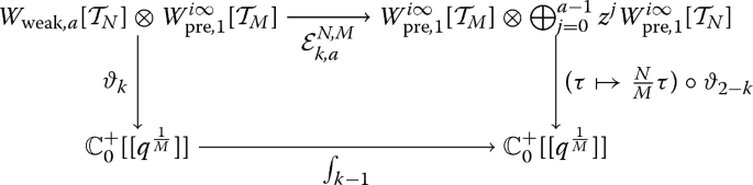
is commutative. Here, \(\int _m\) denotes the m-fold integral as defined in Definition 4.1.

Proof
-
(i)
We show that the map
$$\begin{aligned} {\mathcal {I}}_{k,a}^{M,N} : W_{\mathrm {pre}, 1}^{i\infty }[{\mathcal {T}}_M] \otimes \bigoplus _{j=0}^{a-1} z^{j}W_{\mathrm {pre}, 1}^{i\infty }[{\mathcal {T}}_N] \longrightarrow \bigoplus _{j=0}^{a-1} \partial _z^j W_{\mathrm {pre}, 1}^{i\infty }[{\mathcal {T}}_N] \otimes W_{\mathrm {pre}, 1}^{i\infty }[{\mathcal {T}}_M] \end{aligned}$$with
$$\begin{aligned} x \otimes y = x \otimes \sum _{\ell =0}^{a-1} z^\ell y_\ell \longmapsto N^{k-1} \sum _{\ell =0}^{a-1} N^{-\ell } \partial ^\ell _z {\mathcal {F}}_N^{-1} y_\ell \otimes {\mathcal {F}}_M x \end{aligned}$$is an inverse of \({\mathcal {E}}_{k,a}^{N,M}\). We find for \(\omega \otimes \eta \in \bigoplus _{j=0}^{a-1} \partial _z^j W_{\mathrm {pre}, 1}^{i\infty }[{\mathcal {T}}_N] \otimes W_{\mathrm {pre}, 1}^{i\infty }[{\mathcal {T}}_M]\):
$$\begin{aligned}&{\mathcal {I}}_{k,a}^{M,N}\left( {\mathcal {E}}_{k,a}^{N,M}(\omega \otimes \eta ) \right) = {\mathcal {I}}_{k,a}^{M,N}\left( N^{1-k} {\mathcal {F}}_M^{-1} \eta \otimes \sum _{j=0}^{a-1} (zN)^j {\mathcal {F}}_N \lambda _j \right) \\&\quad = \sum _{j=0}^{a-1} \sum _{\ell =0}^{a-1} N^{j - \ell } \left( \delta _{j,\ell } \partial _z^\ell {\mathcal {F}}_N^{-1} {\mathcal {F}}_N \lambda _j \otimes {\mathcal {F}}_M {\mathcal {F}}_M^{-1} \eta \right) = \sum _{j=0}^{a-1} \left( \partial _z^j \lambda _j \otimes \eta \right) = \omega \otimes \eta . \end{aligned}$$The other way round we see for \(a \otimes b \in W_{\mathrm {pre}, 1}^{i\infty }[{\mathcal {T}}_M] \otimes \bigoplus _{j=0}^{a-1} z^{j}W_{\mathrm {pre}, 1}^{i\infty }[{\mathcal {T}}_N]\):
$$\begin{aligned} {\mathcal {E}}_{k,a}^{N,M}\left( {\mathcal {I}}_{k,a}^{M,N}\left( a \otimes b \right) \right)&= {\mathcal {E}}_{k,a}^{N,M}\left( N^{k-1} \sum _{\ell =0}^{a-1} N^{-\ell } \partial _z^\ell {\mathcal {F}}_N^{-1}b_\ell \otimes {\mathcal {F}}_M a \right) \\&= N^{k-1} N^{1-k} \left( {\mathcal {F}}_M^{-1} {\mathcal {F}}_M x \otimes \sum _{j=0}^{a-1} N^{-j}(zN)^j {\mathcal {F}}_N {\mathcal {F}}_N^{-1} b_j\right) = a \otimes b. \end{aligned}$$ -
(ii)
We prove that the compositions give the same output. Let \(\omega \otimes \eta \in W_{\mathrm {weak},a}[{\mathcal {T}}_N] \otimes W^{i\infty }_{\mathrm {pre},1}[{\mathcal {T}}_M]\) and \(\omega \) be given by
$$\begin{aligned} \omega = \sum _{j=0}^{a-1} \partial ^j \lambda _j, \quad \lambda _0 \in W_N, \lambda _j \in W^{i\infty }_{\mathrm {pre},1}[{\mathcal {T}}_N]. \end{aligned}$$Since \(1 \leqslant a \leqslant k-2\), according to Theorem 4.10 and Remark 4.11 we have that
$$\begin{aligned} \int _{k-1} \vartheta _{k}(\omega \otimes \eta ; \tau ) = \sum _{j=0}^{a-1} N^{1 + j - k} \vartheta _{2-k+j}\left( {\mathcal {F}}_M^{-1} \eta \otimes {\mathcal {F}}_N \lambda _j; \frac{N\tau }{M}\right) . \end{aligned}$$(4.1)On the other hand, we find
$$\begin{aligned} \vartheta _{2-k}\left( {\mathcal {E}}_{k,a}^{N,M}(\omega \otimes \eta ); \tau \right)&= N^{1-k}\vartheta _{2-k}\left( {\mathcal {F}}_M^{-1} \eta \otimes \sum _{j=0}^{a-1} (Nz)^j {\mathcal {F}}_N \lambda _j; \tau \right) \\&= \sum _{j=0}^{a-1} N^{1-k+j}\vartheta _{2-k+j}\left( {\mathcal {F}}_M^{-1} \eta \otimes {\mathcal {F}}_N \lambda _j; \tau \right) . \end{aligned}$$
This proves the theorem. \(\square \)
Before we apply this to several situations we first recall basic facts about Eichler integrals.
Proposition 4.14
Let \(f : {\mathbb {H}}\rightarrow {\mathbb {C}}\) be a holomorphic function with the following properties:
-
(i)
f is periodic and has a Fourier expansion of the form \(f(\tau ) = \sum _{n=1}^\infty a_f(n)q^{n/\lambda }\) with some \(\lambda > 0\).
-
(ii)
There is an integer \(k \geqslant 2\) and a dual function \(f^*\) with a Fourier expansion \(f^*(\tau ) = \sum _{n=1}^\infty a_{f^*}(n)q^{n/\lambda ^*}\) with \(\lambda ^* > 0,\) such that
$$\begin{aligned} f(-1/\tau ) = \tau ^k f^*(\tau ). \end{aligned}$$ -
(iii)
The coefficients \(a_f(n)\) and \(a_{f^*}(n)\) are polynomially bounded, such that the corresponding L-functions \(L(f; s) = \sum _{n=1}^\infty a_f(n)n^{-s}\) and \(L_{f^*}(s)\) converge on some right half plane.
Then the functions \(L_f\) and \(L_{f^*}\) have meromorphic continuations to the entire plane. If we further put
and
we obtain
where
We can easily apply this formalism to the simplest case of Eisenstein series. It is well-known that if \(\chi \) and \(\psi \) are primitive Dirichlet characters modulo \(N_\chi > 1\) and \(N_\psi > 1\) and \(f(\tau ) = E_k(\chi , \psi ; \tau )\) the corresponding L-function is
We assume that both \(\chi \) and \(\psi \) are non-principal. From identity (0.2) and Theorem 4.13 we obtain
Since
where
this combines to
In the sense of Proposition 4.14 we have \(E^*_k(\chi , \psi ; \tau ) = \chi (-1) E_k(\psi , \chi ; \tau )\) and this provides
since \(\chi (-1)^2 = 1\). Now according to Proposition 4.14 we have the functional equation
On the other hand, from Theorem 1.5, we obtain
And this concludes the following theorem.
Theorem 4.15
Let \(k \geqslant 3\) be an integer, \(\chi \) and \(\psi \) be two primitive Dirichlet characters with \(\chi (-1)\psi (-1) = (-1)^k\) and \(f(\tau ) = E_k(\chi , \psi ; \tau )\). We then have the following identity between rational functions:
Proof
With (4.2) and (4.3) we obtain
The claim now follows when dividing by \(\tau ^{k-2}\) and with \(\psi (-1)\chi (-1) = (-1)^k\). \(\square \)
Remark 4.16
Note that Theorem 4.15 will initially work for \(k=2\) as well, since the considered characters all satisfy \(\chi (0) = \psi (0) =0\), so that we may assume that \(\eta \) is weak and has a removable singularity in \(z=0\) in the proof of Eichler duality. So we are allowed to fulfill step (4.1) even if \(k-2 < a\).
Finally, we give a numerical example.
Example 4.17
Put \(k=6\), \(N_\psi = 5\) and \(N_\chi = 7\). Consider the Legendre symbol \(\psi _5\) and the character \(\chi _7\) generated by \(\chi _7(3) = e^{\frac{2\pi i}{3}}\). Note that we have \(\psi _5(-1) = \chi _7(-1) = 1\). With this we obtain the data
With this we calculate
either by numerical calculation or by using the formulas. Again, using direct calculation or Mathematica one sees
References
Berndt, B., Yeap, B.: Explicit evaluations and reciprocity theorems for finite trigonometric sums. Adv. Appl. Math. 29(3), 358–385 (2002)
Berndt, B., Zaharescu, A.: Finite trigonometric sums and class numbers. A. Math. Ann. 330(3), 551–575 (2004)
Bol, G.: Invarianten linearer Differentialgleichungen. Abh. Math. Semin. Univ. Hambg 16, 1–28 (1949)
Chu, W., Marini, A.: Partial fractions and trigonometric identities. Adv. Appl. Math. 23, 115–175 (1999)
Diamantis, N., Rolen, L.: Eichler cohomology and zeros of polynomials associated to derivatives of L-functions (2017). arXiv:1704.02667v1
Franke, J.: A dominated convergence theorem for Eisenstein series. Ann. math. Québec (to appear)
Franke, J.: Dirichlet series with trigonometric coefficients. Integers 21, A23 (2021)
Franke, J.: Rational functions and modular forms. Proc. Am. Math. Soc. 148, 4151–4164 (2020)
Gun, S., Murty, M.R., Rath, P.: Transcendental values of certain Eichler integrals. Bull. Lond. Math. Soc. 43(5), 939–952 (2011)
Hansen, E.R.: A Table of Series and Products. Prentice-Hall, Englewood Cliffs (1975)
Kohnen, W., Zagier, D.: Modular forms with rational periods. In: Rankin, R.A. (ed.) Modular Forms, pp. 197–249. Ellis Horwood, Chichester (1984)
Kontsevich, M., Zagier, D.: Periods, Mathematics Unlimited—2001 and Beyond, pp. 771–808. Springer, Berlin (2001)
Loxton, J.H.: On the determination of Gauss sums, Séminaire Delange-Pisot-Poitou. Théorie des nombres 18(2), 1–12 (1976–1977)
Manin, Y.I.: Local zeta factors and geometries under \({\rm Spec }{{\mathbb{Z}}}\). Izv. Russ. Acad. Sci. 80(4), 123–130 (2016)
Neto, A.F.: Higher order derivatives of trigonometric functions. Stirling numbers of the second kind, and Zeon algebra. J. Integer Seq. 17, 14.9.3 (2014)
Authors' contributions
The author is very grateful to Winfried Kohnen and the anonymous referees for many helpful comments that strongly improved the paper.
Funding
Open Access funding enabled and organized by Projekt DEAL.
Author information
Authors and Affiliations
Corresponding author
Additional information
Publisher's Note
Springer Nature remains neutral with regard to jurisdictional claims in published maps and institutional affiliations.
Rights and permissions
Open Access This article is licensed under a Creative Commons Attribution 4.0 International License, which permits use, sharing, adaptation, distribution and reproduction in any medium or format, as long as you give appropriate credit to the original author(s) and the source, provide a link to the Creative Commons licence, and indicate if changes were made. The images or other third party material in this article are included in the article’s Creative Commons licence, unless indicated otherwise in a credit line to the material. If material is not included in the article’s Creative Commons licence and your intended use is not permitted by statutory regulation or exceeds the permitted use, you will need to obtain permission directly from the copyright holder. To view a copy of this licence, visit http://creativecommons.org/licenses/by/4.0/.
About this article

Cite this article
Franke, J. Rational functions, cotangent sums and Eichler integrals. Res. number theory 7, 23 (2021). https://doi.org/10.1007/s40993-021-00250-4
Received:
Accepted:
Published:
DOI: https://doi.org/10.1007/s40993-021-00250-4