The key role of convexity in some copula constructions

Abstract

We start with some binary (“outer”) copula, apply it to an arbitrary binary (“inner”) copula and its dual (the latter being transformed by some real function) and ask under which conditions the result is again a binary copula. Sufficient convexity conditions for the transformation function and for the “outer” copula (ultramodularity and Schur concavity) are given, thus generalizing the scenarios considered in Klement et al. (J Math Inequal 11(2):361–381, 2017) and Manstavičius and Bagdonas (Fuzzy Sets Syst 354:48–62, 2019). In general, these sufficient conditions are not necessary (and a counterexample is provided), but in some distinguished cases necessary and sufficient conditions can be given. Several well-known families of copulas can be obtained in this way. We also present a few extensions for special “outer”/“inner” copulas and/or transformation functions, as well as some counterexamples.

1 Introduction

Binary quasi-copulas [2, 26] and copulas (introduced in [73], see also [1, 25, 57, 67]) are special aggregation functions [29]. Due to Sklar’s Theorem [18, 73], copulas play a significant role in probability theory [32], especially in dependence modeling [33]. Other areas related to (quasi-)copulas are generalized integration theory [37, 41, 42], decision theory [77], finance [7, 27], preference modeling [9, 13], but also fuzzy logics and the theory of fuzzy sets [10, 30, 63].

Many constructions for (quasi-)copulas based on some given (quasi-)copulas have been proposed, including Archimedean copulas (which are isomorphic transformations of the product copula $\Pi$ or the Fréchet–Hoeffding lower bound W [1, 30, 47, 55, 57, 67]), several types of ordinal sums, based either on the Fréchet–Hoeffding upper bound M (M-ordinal sums) [1, 23, 36, 57, 66, 67], on W (W-ordinal sums) [54], or on $\Pi$ ($\Pi$-ordinal sums) [11, 22, 23, 53, 64, 72], and the product of distorted copulas [34, 46].

In this paper we present sufficient conditions under which a combination of an arbitrary copula and its dual by means of some transformation function on the unit interval and some “outer” copula yields again a copula. This is a significant generalization of the scenarios considered in [35] (where the transformation function coincides with the identity function) and in [48] (where $\Pi$ was chosen as “outer” copula; see also [14, 20, 44]). In general, these sufficient conditions are not necessary (and a counterexample is provided), but in some special cases necessary and sufficient conditions can be given.

In our investigations some distinguished inequalities for real functions play a key role: the convexity [61] of the transformation function, on the one hand, and two variants of the convexity for the “outer” copula, on the other hand: the ultramodularity [49, 50] and the Schur concavity [65] (see also [52, 62]).

Ultramodular real functions can be found in several areas, and under different names. In the case of an n-dimensional domain, ultramodularity can be seen as a version of convexity: under mild regularity assumptions, the set of ultramodular functions coincides with the set of all functions which are both convex in each variable and supermodular [49]. In the special case $n=2$, ultramodularity is just convexity along the main diagonal.

Ultramodular functions have been used in economics, in particular in game theory in the context of convex measure games [3], but they also have applications in multicriteria decision support systems [5]. In mathematical analysis, ultramodular functions appeared for the first time in [76] where they were simply called convex functions (now some authors use the term Wright convexity for them [60]). In statistics, ultramodular functions occur when modeling stochastic orders and positive dependence among random vectors [56, 68] (in this context they are known also as directional convex functions). For more details about ultramodular real functions see [49].

Ultramodular binary copulas are fully characterized by the convexity of their horizontal and vertical sections [38, 49], and they were studied recently in [35, 39]. They describe the dependence structure of stochastically decreasing random vectors, and thus each ultramodular copula is negative quadrant dependent (NQD) [57].

The concepts of Schur convex functions and Schur concave functions (as their duals) were introduced in [65] as variants of the convexity of real functions (see also [62]). For example, each symmetric convex function is Schur convex (and each symmetric concave function is Schur concave). Each Schur concave copula is necessarily symmetric, and each associative copula is Schur concave [24]. Schur convex functions preserve a preorder called majorization [51] and play a role in some related inequalities [69]. An early application was the comparison of incomes, and they also appear in physics, chemistry, political science, engineering, and economics [52].

A simple example of a Schur convex function in several variables is the maximum. The minimum and the product of strictly positive factors are Schur concave, as well as all elementary symmetric functions (again only in the case of strictly positive components) [70, 71]. In the framework of stochastics and aggregation functions [29], the variance and the standard deviation are Schur convex, and the Shannon entropy function, the Rényi entropy function, and the Gini coefficient are examples of Schur concave functions [4, 28, 45, 58, 59].

2 Preliminaries

A (binary) aggregation function [29] is a function $A :[0,1]^2 \rightarrow [0,1]$ which is monotone non-decreasing (in each component) and satisfies the two boundary conditions $A(0,0)=0$ and $A(1,1)=1$.

We often require an aggregation function $A :[0,1]^2 \rightarrow [0,1]$ to be 1-Lipschitz (with respect to the $L^1$-norm), i.e., for all pairs $(x_1,y_1), (x_2,y_2)\in [0,1]^2$,

$$\begin{aligned} |A(x_1,y_1)-A(x_2,y_2)|\leqslant |x_1- x_2| + |y_1 -y_2|. \end{aligned}$$

Given a binary 1-Lipschitz aggregation function $A:[0,1]^2\rightarrow [0,1]$, its dual function $A^*:[0,1]^2\rightarrow [0,1]$ is defined by [29]

$$\begin{aligned} A^*(x,y) = x+y - A(x,y), \end{aligned}$$

and it is also a binary 1-Lipschitz aggregation function.

Each 1-Lipschitz aggregation function A satisfies the inequality $W\leqslant A \leqslant W^*$, where the so-called Fréchet–Hoeffding lower bound$W :[0,1]^2 \rightarrow [0,1]$ is given by , and its dual $W^*$ by .

A (binary) quasi-copula$Q:[0,1]^2 \rightarrow [0,1]$ is a 1-Lipschitz aggregation function with annihilator 0 and neutral element 1, i.e., we have $Q(0,x)=Q(x,0)=0$ and $Q(1,x)=Q(x,1)=x$ for all $x\in [0,1]$ (see [2, 26]).

A 1-Lipschitz aggregation function $A :[0,1]^2\rightarrow [0,1]$ is a quasi-copula if and only if $A(0,1)=A(1,0)=0$ (see [43]) or, equivalently, if and only if $A\leqslant M$, where the Fréchet–Hoeffding upper bound M is given by .

To simplify some formulas, we shall occasionally also use the infix notations for the component-wise minimum and maximum of ${{\mathbf {x}}} ,{{\mathbf {y}}} \in \mathbb {R}^n$: for and for .

A (binary) copula $C:[0,1]^2\rightarrow [0,1]$ (see [25, 32, 57, 73]) is a supermodular quasi-copula, i.e., for all ${{\mathbf {x}}} ,{{\mathbf {y}}} \in [0,1]^2$,

In an equivalent definition, a function $C:[0,1]^2\rightarrow [0,1]$ is a binary copula if and only if $C(0,x)=C(x,0)=0$ and $C(1,x)=C(x,1)=x$ for all $x\in [0,1]$, and if C is 2-increasing, i.e., for all $x_1,x_2,y_1,y_2\in [0,1]$ with $x_1\leqslant x_2$ and $y_1\leqslant y_2$ for the volume $V_C$ of the rectangle ,

Obviously, each copula is a quasi-copula but not vice versa, and each quasi-copula Q satisfies

$$\begin{aligned} W\leqslant Q\leqslant M. \end{aligned}$$

Observe that, for any quasi-copula Q, 1 is not a neutral element of $Q^*$, so the dual of a quasi-copula is never a quasi-copula (nor is the dual of a copula a copula).

In this paper, the convexity [61] of real functions and two other properties related to distinguished inequalities for real functions (in our case, for binary copulas) will play a major role: the ultramodularity [49] and the Schur concavity [65].

Consider an n-dimensional cuboid $A\subseteq \mathbb {R}^n$ and recall that a function $f:A\rightarrow \mathbb {R}$ is called convex whenever for all ${{\mathbf {x}}} ,{{\mathbf {y}}} \in A$ and for all $\lambda \in [0,1]$.

If $A\subseteq \mathbb {R}^n$ then a function $f:A\rightarrow \mathbb {R}$ is called ultramodular [49] if its increments are monotone non-decreasing, i.e., if for all ${{\mathbf {x}}} ,{{\mathbf {y}}} \in A$ with ${{\mathbf {x}}} \leqslant {{\mathbf {y}}}$ and all ${{\mathbf {h}}} \geqslant \mathbf {0}$ such that ${{\mathbf {x}}} +{{\mathbf {h}}} ,{{\mathbf {y}}} +{{\mathbf {h}}} \in A$,

$$\begin{aligned} f({{\mathbf {x}}} +{{\mathbf {h}}} )- f({{\mathbf {x}}} ) \leqslant f({{\mathbf {y}}} +{{\mathbf {h}}} ) - f({{\mathbf {y}}} ). \end{aligned}$$

Therefore, a binary copula $C:[0,1]^2\rightarrow [0,1]$ is ultramodular [35, 38, 39] if and only if for all ${{\mathbf {x}}} ,{{\mathbf {y}}} ,{{\mathbf {z}}} \in [0,1]^2$ satisfying ${{\mathbf {x}}} +{{\mathbf {y}}} +{{\mathbf {z}}} \in [0,1]^2$,

$$\begin{aligned} C({{\mathbf {x}}} +{{\mathbf {y}}} +{{\mathbf {z}}} )+ C({{\mathbf {x}}} ) \geqslant C({{\mathbf {x}}} +{{\mathbf {y}}} ) + C({{\mathbf {x}}} +{{\mathbf {z}}} ). \end{aligned}$$

Note that, as a consequence of [49, Corollary 4.1] and [38, Proposition 2.7], ultramodular copulas are just copulas with convex horizontal and vertical sections.

Among the three basic copulas, i.e., the Fréchet–Hoeffding bounds W and M and the product copula $\Pi :[0,1]^2\rightarrow [0,1]$ given by $\Pi (x,y)=x{\cdot }y$, only W and $\Pi$ are ultramodular. However, the restriction of the upper Fréchet–Hoeffding bound M to the upper left triangle $\Delta =\{(x,y)\in [0,1]^2 \,{|}\, x \leqslant y \}$ is ultramodular.

If $C:[0,1]^2\rightarrow [0,1]$ is an Archimedean copula [57] and if its additive generator $t:[0,1]\rightarrow [{0,\infty }]$ is two times differentiable, then from [39, Theorem 3.1] (compare also [6]) we know that C is an ultramodular copula if and only if the function ${1}/{t'}:[0,1]\rightarrow [{0,\infty }]$ is convex.

Considering, for example, the family of Clayton copulas [57] generated by the family defined by , we see that the corresponding Archimedean copulas are ultramodular if and only if $\lambda >0$, i.e., exactly the nilpotent Clayton copulas are ultramodular.

The next distinguished property of binary copulas which will be crucial in our work, the Schur concavity [65], is a special type of monotonicity in the sense that it reverses majorization [51].

Consider a pair ${{\mathbf {x}}} =(x_1,x_2)\in \mathbb {R}^2$ and assign to it a pair $\smash {{{\mathbf {x}}} ^{\downarrow }=(x_1^{\downarrow },x_2^{\downarrow })\in \mathbb {R}^2}$ which has the same components, but sorted in descending order, i.e., $\smash {x_1^{\downarrow }\geqslant x_2^{\downarrow }}$. Given two pairs ${{\mathbf {y}}} =(y_1,y_2)\in \mathbb {R}^2$ and ${{\mathbf {x}}} =(x_1,x_2)\in \mathbb {R}^2$, then ${{\mathbf {y}}}$ is said to majorize ${{\mathbf {x}}}$ (in symbols ${{\mathbf {y}}} \succ {{\mathbf {x}}}$) if¹

$$\begin{aligned} \smash {x_1+ x_2= y_1+y_2 \quad \text {and}\quad y_1^{\downarrow } \geqslant x_1^{\downarrow }}. \end{aligned}$$

Note that $\succ$ is not a partial order on $\mathbb {R}^2$ because it is not antisymmetric: from ${{\mathbf {y}}} \succ {{\mathbf {x}}}$ and ${{\mathbf {x}}} \succ {{\mathbf {y}}}$ we only can conclude that ${{\mathbf {x}}}$ and ${{\mathbf {y}}}$ have the same components, but not necessarily in the same order.

If $A\subseteq \mathbb {R}^2$ then a function $f:A\rightarrow \mathbb {R}$ is Schur convex [65] if f preserves majorization, i.e., ${{\mathbf {y}}} \succ {{\mathbf {x}}}$ implies $f({{\mathbf {y}}} )\geqslant f({{\mathbf {x}}} )$. A function $f:A\rightarrow \mathbb {R}$ is said to be Schur concave if it reverses majorization, i.e., its negation $(-f):A\rightarrow \mathbb {R}$ is Schur convex.

In other words, a function $f:[0,1]^2\rightarrow [0,1]$ is Schur concave if and only if, for all $(x,y), (u,v) \in [0,1]^2$ with $x+y = u+v$ and , the inequality $f(x,y) \leqslant f(u,v)$ holds.

Equivalently, a function $f:[0,1]^2\rightarrow [0,1]$ is Schur concave if and only if, for all $(x,y) \in [0,1]^2$ and all $\lambda \in [0,1]$,

Clearly, the three basic copulas W, $\Pi$ and M are Schur concave, as well as each associative copula. Observe that each Schur concave copula is symmetric [24].

In our context the Schur concavity of a copula $D:[0,1]^2\rightarrow [0,1]$ is only required on the upper left triangle $\Delta =\{(x,y)\in [0,1]^2 \,{|}\, x \leqslant y \}$, i.e., we only need the Schur concavity of the restriction $D\mathord {\upharpoonright }_{\Delta }:\Delta \rightarrow [0,1]$ of D to $\Delta$. This is equivalent with saying that for all $(x,y) \in \Delta$ and for all $\varepsilon > 0$ with $(x+\varepsilon ,y-\varepsilon ) \in \Delta$,

$$\begin{aligned} D(x,y) \leqslant D(x+\varepsilon ,y-\varepsilon ). \end{aligned}$$

Observe that symmetric copulas which are Schur concave on $\Delta$ are necessarily Schur concave (on the whole unit interval). However, a copula which is Schur concave on $\Delta$ need not be symmetric: for instance, the copula $D:[0,1]^2\rightarrow [0,1]$ given by

is not symmetric (and, therefore, not Schur concave), but the restriction $D\mathord {\upharpoonright }_{\Delta }$ of D to $\Delta$ coincides with $\Pi \mathord {\upharpoonright }_{\Delta }$, so D is Schur concave on $\Delta$.

3 Main result

We shall deal in this paper with several classes of monotone functions from one real interval to another:

and the analogously defined classes

$$\begin{aligned} \mathscr {M}_{\mathrm {inc,conc}}\bigl ([{c,d}]^{[{a,b}]}\bigr ), \quad \mathscr {M}_{\mathrm {dec,conv}}\bigl ([{c,d}]^{[{a,b}]}\bigr )\quad \text {and}\quad \mathscr {M}_{\mathrm {dec,conc}}\bigl ([{c,d}]^{[{a,b}]}\bigr ), \end{aligned}$$

where the subscript “$\text {dec}$” stands for “monotone non-increasing” and “conc” for “concave”.

We also shall work with the class of 1-Lipschitz functions from the unit interval $[0,1]$ into some real interval $[{c,d}]$ with $c\leqslant 1\leqslant d$:

Lemma 3.1

Let $f:[0,1]\rightarrow [0,1]$ be a function with . Then $f\in {\mathscr {L}}\bigl ([0,1]^{[0,1]}\bigr )$ if and only if $f\geqslant \mathrm{id}_{[0,1]}$.

Proof

Assume that . If $f(1)=1$ and f violates $f\geqslant \mathrm{id}_{[0,1]}$, i.e., if we have $f(x_0)<x_0$ for some $x_0\in \big ]0,1\big [$ then f cannot be 1-Lipschitz because of $\smash {\tfrac{f(1)-f(x_0)}{1-x_0}>\tfrac{1-x_0}{1-x_0} = 1}$.

Conversely, assume $f\geqslant \mathrm{id}_{[0,1]}$. Then obviously $f(1)=1$. If f is not 1-Lipschitz, i.e., there exist $x_0,y_0\in \big ]0,1\big [$ with $x_0 < y_0$ such that $f(y_0) = f(x_0) + k(y_0-x_0)$ for some $k > 1$, then, because of the convexity of f, we have $1= f(1) \geqslant f(x_0) + k (1-x_0)$, implying $1- f(x_0) \geqslant k(1-x_0) > 1-x_0$, i.e., $f(x_0) < x_0$, contradicting the assumption $f\geqslant \mathrm{id}_{[0,1]}$. $\square$

To further simplify our notations, we put

Because of Lemma 3.1, $\smash {{\mathscr {F}}\bigl ([0,1]^{[0,1]}\bigr )}$ consists of all the functions $f:[0,1]\rightarrow [0,1]$ which are monotone non-decreasing, convex, and satisfy $f\geqslant \mathrm{id}_{[0,1]}$.

Now let us start with some function $f:[0,1]\rightarrow [0,1]$ and some binary copula $D:[0,1]^2\rightarrow [0,1]$ and consider the composite function $D(C,f(C^*)):[0,1]^2\rightarrow [0,1]$ given by

$$\begin{aligned} D(C,f(C^*))(x,y)= D(C(x,y),f(C^*(x,y))). \end{aligned}$$

(3.1)

Note that in the special case $f=\mathrm{id}_{[0,1]}$ formula (3.1) reduces to

$$\begin{aligned} D(C,C^*)(x,y) = D(C(x,y),C^*(x,y)). \end{aligned}$$

(3.2)

We want to know under which conditions, for each binary copula $C:[0,1]^2\rightarrow [0,1]$, the composite function $D(C,f(C^*))$ defined by (3.1) is also a binary copula. In this context, we also will refer to f as “transformation function”, to D as “outer” and to C as “inner” copula.

For some particular choices of the transformation function f (namely, $f=\mathrm{id}_{[0,1]}$) and the outer copula D (namely, $D=\Pi$ and $D=M$) we have the following results, some of which are already known from the literature.

The first of these results deals with the special case $f=\mathrm{id}_{[0,1]}$ (compare the earlier results in [14, Theorem 3.1] and [44, Theorem 1]).

Theorem 3.2

([35, Theorem 3.1]) Let $D:[0,1]^2\rightarrow [0,1]$ be a binary copula which is ultramodular and Schur concave on the upper left triangle $\Delta$ of $[0,1]^2$. Then, for each binary copula $C:[0,1]^2\rightarrow [0,1]$, the composite function $D(C,C^*):[0,1]^2\rightarrow [0,1]$ given by (3.2) is a binary copula.

The second of these results considers the case $D=\Pi$ (compare [19, Lemma 3.1, (3.4)]). Observe that in this case the original result in [48] was given for functions of the form $\Pi (C,g(1-C^*))$, where $g(x)=f(1-x)$.

Theorem 3.3

([48, Theorem 2]) Let $f:[0,1]\rightarrow [0,1]$ be a function. Then the following are equivalent:

• (i) $\smash {f\in {\mathscr {F}}\bigl ([0,1]^{[0,1]}\bigr )}$;

• (ii) for each binary copula $C:[0,1]^2\rightarrow [0,1]$ the composite function

  

  given by (3.1) is a binary copula.

As far as we know, the third of these results (for the special case $D=M$) is new.

Proposition 3.4

Let $f:[0,1]\rightarrow [0,1]$ be a function. Then the following are equivalent:

• (i) $f\geqslant \mathrm{id}_{[0,1]}$;

• (ii) for each binary copula $C:[0,1]^2\rightarrow [0,1]$ the composite function

  $$\begin{aligned} M(C,f(C^*)):[0,1]^2\rightarrow [0,1]\end{aligned}$$

  given by (3.1) is a binary copula.

Proof

For each copula we have $C\leqslant C^*$. If $f\geqslant \mathrm{id}_{[0,1]}$ then $C\leqslant f(C^*)$ and, subsequently, $M(C,f(C^*))=C$, i.e., $M(C,f(C^*))$ is a copula. This shows that (i) implies (ii).

For the converse, assume that, for each copula C, also $M(C,f(C^*))$ is a copula and that there is an $x_1\in \big ]0,1\big [$ with $f(x_1)<x_1$. Now fix $C=M$ and write briefly $E=M(M,f(M^*))$, i.e.,

and, in particular, for all $x\in [0,1]$.

Then , i.e., $f(1) = 1$, and $E(x_1,x_1) = f(x_1) < x_1$. Taking into account the continuity and the monotonicity of the copula E, $f(1)=1$ implies that there is an $x_2\in \big ]{x_1,1}\big [$ such that $f(x_1)<f(x_2)\leqslant x_1$. Then we get for the volume $V_E$,

$$\begin{aligned} V_E\bigl ([{x_1,x_2}]^2\bigr ) = E(x_2,x_2) + E(x_1,x_1) - 2 E(x_1,x_2) = f(x_1) - f(x_2) < 0, \end{aligned}$$

i.e., E is not 2-increasing, which is a contradiction to our assumptions. $\square$

Our main result generalizes these results and provides sufficient conditions for the transformation function f and the outer copula D such that, for each copula C, also the function $D(C,f(C^*))$ is a copula.

Theorem 3.5

Let $f:[0,1]\rightarrow [0,1]$ be a function and $D:[0,1]^2\rightarrow [0,1]$ be a binary copula. If $\smash {f\in {\mathscr {F}}\bigl ([0,1]^{[0,1]}\bigr )}$ and if D is both ultramodular and Schur concave on the upper left triangle $\Delta$ of the unit square then, for each binary copula $C:[0,1]^2\rightarrow [0,1]$, the composite function $D(C,f(C^*))$ given by (3.1) is a binary copula.

Proof

Fix an arbitrary binary copula C and a binary copula D which is ultramodular and Schur concave on $\Delta$, and write briefly $E=D(C,f(C^*))$, i.e., for all $(x,y)\in [0,1]^2$,

$$\begin{aligned} E(x,y)=D(C(x,y),f(C^*(x,y))). \end{aligned}$$

(3.3)

We first show that the assumptions in Theorem 3.5 imply that E satisfies both boundary conditions of copulas. For each $x\in [0,1]$ we have

$$\begin{aligned} E(x,0) = D(C(x,0),f(C^*(x,0))) = D(0,f(C^*(x,0)))= 0 \end{aligned}$$

and, as $f(1)=1$, we also get

$$\begin{aligned} E(x,1) = D(C(x,1),f(x+1-C(x,1))) = D(x,1)=x. \end{aligned}$$

Similarly, we get $E(0,x)=0$ and $E(1,x)=x$, i.e., E is grounded with neutral element 1.

Secondly, we check that E is 2-increasing. Fix $(x,y)\in \big ]0,1\big [^2$, $\varepsilon \in \big ]{0,1-x}\big [$ and $\delta \in \big ]{0,1-y}\big [$ and consider the rectangle

We have to show that

$$\begin{aligned} V_E(R)= E(x+\varepsilon ,y+\delta ) - E(x,y+\delta ) + E(x,y) - E(x+\varepsilon ,y) \geqslant 0. \end{aligned}$$

(3.4)

Define the numbers $\alpha$, $\beta$, $\gamma \in [0,1]$ by

$$\begin{aligned} \begin{aligned} \alpha&= C(x,y+\delta ) - C(x,y),\\ \beta&= C(x+\varepsilon ,y) - C(x,y), \\ \gamma&= C(x+\varepsilon ,y+\delta ) - C(x,y). \end{aligned} \end{aligned}$$

(3.5)

From the monotonicity and the 1-Lipschitz property of C we get $0\leqslant \alpha \leqslant \delta$ and $0\leqslant \beta \leqslant \varepsilon$. The 2-increasingness of C implies $\alpha + \beta \leqslant \gamma$, and the 1-Lipschitz property gives $\gamma \leqslant \delta + \varepsilon$.

Using (3.3) and (3.5), we can rewrite (3.4) as

$$\begin{aligned} \begin{aligned} V_E(R)&= D\bigl (C(x,y) + \gamma , f(C^*(x,y) + \delta +\varepsilon - \gamma )\bigr )\\&\qquad \qquad -\, D\bigl (C(x,y)+\alpha ,f(C^*(x,y)+ \delta - \alpha )\bigr )\\&\qquad \qquad +\, D\bigl (C(x,y),f(C^*(x,y))\bigr )\\&\qquad \qquad -\,D\bigl (C(x,y) + \beta , f(C^*(x,y) + \varepsilon - \beta )\bigr ). \end{aligned} \end{aligned}$$

(3.6)

To simplify the notation put $u= C(x,y)$ and $v= C^*(x,y)$. Then (3.6) may be rewritten as

$$\begin{aligned} \begin{aligned} V_E(R)&= D(u+\gamma , f(v+\delta + \varepsilon - \gamma )) - D(u + \alpha , f(v + \delta - \alpha ))\\&\qquad \qquad \qquad \qquad +\, D(u, f(v)) - D(u+\beta , f(v+ \varepsilon - \beta )). \end{aligned} \end{aligned}$$

(3.7)

Identifying, as usual, two-dimensional vectors with points in $[0,1]^2$ and putting

$$\begin{aligned} P_1&= (p_{11},p_{12})=(u,f(v)), \end{aligned}$$

(3.8)

$$\begin{aligned} P_2&= (p_{21},p_{22})=(u+\beta , f(v+ \varepsilon - \beta )),\end{aligned}$$

(3.9)

$$\begin{aligned} P_3&= (p_{31},p_{32})=(u + \alpha , f(v + \delta - \alpha )),\end{aligned}$$

(3.10)

$$\begin{aligned} P_4&= (p_{41},p_{42})=(u+\gamma , f(v+\delta + \varepsilon - \gamma )), \end{aligned}$$

(3.11)

the volume $V_E(R)$ in (3.7) can be written as

$$\begin{aligned} V_E(R)= D(P_4) - D(P_3) + D(P_1) - D(P_2). \end{aligned}$$

(3.12)

If we replace in (3.8)–(3.11) the values u and v by their original meaning, i.e.,

$$\begin{aligned} P_1&=\bigl (C(x,y), f(C^*(x,y))\bigr ), \\ P_2&= \bigl (C(x+\varepsilon ,y),f(C^*(x+\varepsilon ,y))\bigr ), \\ P_3&= \bigl (C(x,y+\delta ), f(C^*(x, y+ \delta ))\bigr ),\\ P_4&= \bigl (C(x+\varepsilon ,y+\delta ), f(C^*(x+\varepsilon ,y+\delta ))\bigr ), \end{aligned}$$

and take into account that for all $(a,b)\in [0,1]^2$,

$$\begin{aligned} 0\leqslant C(a,b)\leqslant C^*(a,b)\leqslant f(C^*(a,b))\leqslant 1, \end{aligned}$$

we see that $\{P_1, P_2, P_3,P_4\}\subset \Delta$.

Consider also the point $P_5$ such that $P_1, P_2, P_3$, and $P_5$ are the vertices of a parallelogram, i.e.,

$$\begin{aligned} P_5 = (p_{51},p_{52})=\bigl (u + \alpha + \beta , f(v + \varepsilon - \beta ) + f(v + \delta - \alpha ) - f(v)\bigr ), \end{aligned}$$

(3.13)

and the point $P_6$ given by

$$\begin{aligned} P_6 = (p_{61},p_{62}) = \bigl (u + \alpha + \beta , f(v + \delta + \varepsilon - \gamma ) + \gamma - \alpha - \beta \bigr ). \end{aligned}$$

(3.14)

Then, from the convexity of f it follows that

$$\begin{aligned} f(v + \delta - \alpha ) - f(v) \leqslant f(v + \varepsilon - \beta + \delta - \alpha ) - f(v + \varepsilon - \beta ), \end{aligned}$$

(3.15)

and the 1-Lipschitz property of f (see Lemma 3.1) yields

$$\begin{aligned} f(v + \delta + \varepsilon - \alpha - \beta ) - f(v + \delta + \varepsilon - \gamma ) \leqslant \gamma - \alpha - \beta . \end{aligned}$$

(3.16)

Adding the left- and right-hand sides of the inequalities (3.15) and (3.16) and canceling the expression $f(v + \varepsilon - \beta + \delta - \alpha )$ on both sides of the sum, we obtain

$$\begin{aligned} f(v + \delta - \alpha ) - f(v) - f(v + \delta + \varepsilon - \gamma ) \leqslant - f(v + \varepsilon - \beta ) + \gamma - \alpha - \beta , \end{aligned}$$

which yields

$$\begin{aligned} f(v + \delta + \varepsilon + \delta - \gamma ) + \gamma - \alpha - \beta \geqslant f(v + \delta - \alpha ) + f(v + \varepsilon - \beta ) - f(v), \end{aligned}$$

i.e., $p_{62}\geqslant p_{52}$ (see (3.13) and (3.14)). Since $p_{51}=p_{61}$, we have

$$\begin{aligned} P_6 = (p_{61},p_{62}) \geqslant (p_{51},p_{52}) = P_5. \end{aligned}$$

(3.17)

In order to complete the check that E is 2-increasing we distinguish the following three cases:

Case 1: $\{P_5,P_6\}\subset \Delta$ (see Fig. 1 (left)).

Since D is ultramodular on $\Delta$ we may apply [35, (2.7)] to the parallelogram with the vertices $P_1,P_2,P_3$, and $P_5$, and we obtain

$$\begin{aligned} D(P_5) - D(P_3) + D(P_1)- D(P_2) \geqslant 0. \end{aligned}$$

(3.18)

From (3.17) and the monotonicity of D we get

$$\begin{aligned} D(P_6) \geqslant D(P_5). \end{aligned}$$

(3.19)

Fig. 1

Proof of Theorem 3.5: the cases $\{P_5,P_6\}\subseteq \Delta$ (left), and $P_5\in \Delta$ and $P_6\notin [0,1]^2$ (right)

Finally, we want to show that $D(P_4) \geqslant D(P_6)$. Clearly (see (3.11) and (3.14)) we have

$$\begin{aligned} p_{41} + p_{42} = u + \gamma + f(v + \delta + \varepsilon - \gamma ) = p_{61} + p_{62}. \end{aligned}$$

Note that for each point $P=(x,y)$ on the line segment connecting $P_4$ and $P_6$ we have

$$\begin{aligned} x+y= u + \gamma + f(v + \delta + \varepsilon - \gamma ). \end{aligned}$$

The slope of this line equals $-1$, i.e., it is orthogonal to the main diagonal of the unit square. Moreover,

Hence, from the Schur concavity of D on $\Delta$ (see [35, p. 367, lines 9–11]), it follows that

$$\begin{aligned} D(P_4) \geqslant D(P_6). \end{aligned}$$

(3.20)

Combining (3.19) and (3.20) we have $D(P_4) \geqslant D(P_5)$, and (3.12) and (3.18) imply that

$$\begin{aligned} V_E(R)&= D(P_4) - D(P_3) + D(P_1) - D(P_2) \\&\geqslant D(P_5) - D(P_3) + D(P_1) - D(P_2) \geqslant 0, \end{aligned}$$

showing that E is 2-increasing in this case.

Case 2: $P_5\in \Delta$ and $P_6\notin [0,1]^2$ (as shown in Fig. 1 (right)).

Consider two additional points: $Q_1$ is the common point of the upper border $l_u$ of the unit square (i.e., the line segment from (0, 1) to (1, 1)) and of the line connecting $P_4$ and $P_6$. $Q_2$ is the intersection point of $l_u$ and the line connecting $P_5$ and $P_6$ (see Fig. 1 (right)). Clearly, we have

$$\begin{aligned} Q_1&= (q_{11},q_{12}) = (f(v + \delta + \varepsilon - \gamma ) + u + \gamma -1, 1),\\ Q_2&= (q_{21},q_{22}) = (u + \alpha + \beta , 1). \end{aligned}$$

Considering the points $Q_2$ and $P_5$, on the one hand, and $Q_1$ and $Q_2$, on the other hand, the monotonicity of D implies

$$\begin{aligned} D(Q_2) \geqslant D(P_5)\quad \text {and}\quad D(Q_1) \geqslant D(Q_2). \end{aligned}$$

(3.21)

Again, for all points $P=(x,y)$ on the line segment connecting $P_4$ and $P_6$ (in particular, for $P_4$ and $Q_1$) we have $x+y= f(v + \delta + \varepsilon - \gamma ) + u + \gamma$. Moreover, we obtain $\min (p_{41}, p_{42})= u + \gamma \geqslant f(v + \delta + \varepsilon - \gamma ) + u + \gamma -1 = \min (q_{11}, q_{12})$, and the Schur concavity of D on $\Delta$ (compare [35]) allows us to conclude that $D(P_4) \geqslant D(Q_1)$.

Summarizing, we have $D(P_4) \geqslant D(P_5)$ because of (3.21), and (3.12) and (3.18) imply

$$\begin{aligned} V_E(R)&= D(P_4) - D(P_3) + D(P_1) - D(P_2) \\&\geqslant D(P_5) - D(P_3) + D(P_1) - D(P_2) \geqslant 0, \end{aligned}$$

showing that E is 2-increasing in this case.

Case 3: $P_5\notin [0,1]^2$ (as visualized in Fig. 2).

Fig. 2

Proof of Theorem 3.5: the case $P_5\notin \Delta$

First of all, observe that $P_6\notin [0,1]^2$ because of (3.17). We consider four additional points $Q_3,Q_4,Q_5$, and $Q_6$ as follows:

• $Q_3=(q_{31},q_{32})$ is the intersection point of the upper border $l_u$ of the unit square and the line connecting the points $P_3$ and $P_5$.

• $Q_4=(q_{41},q_{42})$ is the common point of $l_u$ and the line connecting the points $P_2$ and $P_5$.

• $Q_5=(q_{51},q_{52})$ is, together with the points $P_1,P_3$ and $Q_3$, the vertex of a parallelogram, i.e., $(q_{51},q_{52}) = (p_{11},p_{12}) + (q_{31},q_{32}) - (p_{31},p_{32})$.

• $Q_6=(q_{61},q_{62})$ is, together with the points $P_5,Q_3$ and $Q_4$, the vertex of a parallelogram, i.e., $(q_{61},q_{62}) = (q_{41},q_{42}) + (q_{31},q_{32}) - (p_{51},p_{52})$.

Putting

$$\begin{aligned} S_E^{(1)}(R)&= D(Q_3) + D(P_1) - D(P_3) - D(Q_5),\\ S_E^{(2)}(R)&= D(Q_4) + D(Q_5) - D(Q_6) - D(P_2),\\ S_E^{(3)}(R)&= D(P_4) - D(Q_1),\\ S_E^{(4)}(R)&= D(Q_1) - D(Q_4) - D(Q_3) + D(Q_6), \end{aligned}$$

we obtain

$$\begin{aligned} V_E(R)&= D(P_4) - D(P_3) + D(P_1) - D(P_2)\\&= S_E^{(1)}(R) + S_E^{(2}(R) + S_E^{(3)}(R) + S_E^{(4)}(R). \end{aligned}$$

Without going into details, we have $S_E^{(1)}(R)\geqslant 0$ and $S_E^{(2)}(R) \geqslant 0$ because of the ultramodularity of D on $\Delta$, and $S_E^{(3)}(R) \geqslant 0$ because of the Schur concavity of D on $\Delta$. It remains to be shown that $S_E^{(4)}(R) \geqslant 0$.

Recalling $Q_6 = (q_{61},q_{62})$, there exist $\lambda _1, \lambda _2 >0$ such that $Q_3 = (q_{61}+\lambda _1,1)$ and $Q_4 = (q_{61}+ \lambda _2, 1)$. From $P_5 = (q_{31},q_{32}) + (q_{41},q_{42}) - (q_{61},q_{62})$ we can derive that $P_5 = (q_{61} + \lambda _1 + \lambda _2,2-q_{62})$, i.e., there is some $\lambda _3 >0$ such that

$$\begin{aligned} P_6 = (q_{61}+ \lambda _1 + \lambda _2,2-q_{62} + \lambda _3). \end{aligned}$$

The coordinates of $Q_1$ satisfy the equation $q_{11} - p_{61} + q_{12} - p_{62} = 0$ because the line connecting $P_6$ and $Q_1$ is orthogonal to the main diagonal of the unit square, i.e., $Q_1 = (q_{61} + 1 - q_{62} + \lambda _1 + \lambda _2 + \lambda _3, 1)$. Since the Fréchet–Hoeffding lower bound W is the smallest copula, i.e., $D \geqslant W$, we have

which means that E is 2-increasing also in this case, thus completing the proof. $\square$

Remark 3.6

As a consequence of Proposition 3.4, the condition $f\in {\mathscr {F}}\bigl ([0,1]^{[0,1]}\bigr )$ is not necessary for obtaining a copula $D(C,f(C^*))$ for each copula C: the copula M is both ultramodular and Schur concave on $\Delta$, and for the function $f_0:[0,1]\rightarrow [0,1]$ given by we have $f_0\notin {\mathscr {F}}\bigl ([0,1]^{[0,1]}\bigr )$ because $f_0$ is neither monotone non-decreasing nor convex nor 1-Lipschitz; however, $f_0\geqslant \mathrm{id}_{[0,1]}$ holds and $M(C,f_0(C^*))=C$ is a copula.

If $f:[0,1]\rightarrow [0,1]$ is a function and $D:[0,1]^2\rightarrow [0,1]$ is a copula then Example 3.7 shows that none of the following five properties can be omitted in the hypotheses of Theorem 3.5 (recall that the joint validity of [f1]–[f3] is equivalent to $f\in {\mathscr {F}}\bigl ([0,1]^{[0,1]}\bigr )$ because of Lemma 3.1) if we want that, for each copula C, also $D(C,f(C^*))$ is a copula:

[D1]::

D is ultramodular on $\Delta$;

[D2]::

D is Schur concave on $\Delta$;

[f1]::

f is monotone non-decreasing;

[f2]::

f is convex;

[f3]::

$f\geqslant \mathrm{id}_{[0,1]}$.

Example 3.7

Consider the five properties [D1]–[D2] and [f1]–[f3] given above.

• (i) The binary copula $D_1=M\text {-}(\langle 1/2,1,W\rangle )$ given in [35, Example 4.1 (ii)] violates [D1] and satisfies [D2], and the function $f_1=\mathrm{id}_{[0,1]}$ satisfies [f1]–[f3], and for $C_1=\Pi$ the function $D_1(C_1,f_1(C_1^*))$ is not a copula.

• (ii) The binary copula given in [35, Example 4.1 (i)] satisfies [D1] and violates [D2], and the function $f_2=\mathrm{id}_{[0,1]}$ satisfies [f1]–[f3], and for the copula $C_2=M\text {-}(\langle 1/4,{13}/{24},W\rangle )$ given in [35, Example 4.1 (i)] the function $D_2(C_2,f_2(C_2^*))$ is not a copula.

• (iii) The copula $D_3=\Pi$ satisfies the properties [D1] and [D2], and the function $f_3:[0,1]\rightarrow [0,1]$ given by violates [f1] and satisfies [f2] and [f3], and for $C_3=M$ the function $D_3(C_3,f_3(C_3^*))$ is not monotone non-decreasing and, therefore, not a copula.

• (iv) The copula $D_4=\Pi$ satisfies the properties [D1] and [D2], and the function $f_4:[0,1]\rightarrow [0,1]$ given by satisfies [f1] and [f3] and violates [f2], and for $C_4=\Pi$ the function $D_4(C_4,f_4(C_4^*))$ is not a copula because of

  

• (v) The copula $D_5=\Pi$ satisfies the properties [D1] and [D2], and the function $f_5:[0,1]\rightarrow [0,1]$ given by $f_5(x)=x^2$ satisfies [f1]–[f2] but violates [f3], and for $C_5=\Pi$ the function $D_5(C_5,f_5(C_5^*))$ is not a copula because of

  

One might argue that, instead of $D(C,f(C^*))$ as in Theorem 3.5, also a transformation $g:[0,1]\rightarrow [0,1]$ of the first coordinate could be considered, i.e., composite functions of the type $D(g(C),f(C^*))$. However, if the result $D(g(C),f(C^*))$ should be a copula and, subsequently, 1 its neutral element, this immediately forces g to coincide with the identity function.

It is remarkable that the construction of $D(C,f(C^*))$ in Theorem 3.5 preserves both the ultramodularity and the Schur concavity on $\Delta$ of the copula C (thus generalizing [35, Proposition 3.2]).

Proposition 3.8

Let $C,D:[0,1]^2\rightarrow [0,1]$ be binary copulas, assume that D is ultramodular and Schur concave on $\Delta$, and let $f\in {\mathscr {F}}\bigl ([0,1]^{[0,1]}\bigr )$. Then we have:

• (i) If the copula C is Schur concave on $\Delta$ then also the copula $D(C,f(C^*))$ is Schur concave on $\Delta$.

• (ii) If the copula C is ultramodular on $\Delta$ then also the copula $D(C,f(C^*))$ is ultramodular on $\Delta$.

Proof

In order to show (i) assume that the copula C is Schur concave on $\Delta$, and let us briefly write, as in (3.3), $E=D(C,f(C^*))$. Then for all $(x,y)\in \Delta$ and for all $\alpha \in \bigl [0, \min \bigl (1-x,y,\frac{y-x}{2}\bigr )\bigr ]$ we obtain $C(x+\alpha ,y-\alpha ) \geqslant C(x,y)$, i.e., we have that $C(x+\alpha ,y-\alpha ) = C(x,y) + \beta$ for some $\beta \geqslant 0$. Hence,

$$\begin{aligned} \begin{aligned} E(x+\alpha ,y-\alpha )&= D\bigl (C(x+\alpha ,y-\alpha ), f(C^*(x+\alpha ,y-\alpha ))\bigr )\\&= D\bigl (C(x,y)+\beta ,f(x+y-C(x,y)-\beta )\bigr ). \end{aligned} \end{aligned}$$

(3.22)

Since $f\in {\mathscr {F}}\bigl ([0,1]^{[0,1]}\bigr )$, f is 1-Lipschitz, we have

$$\begin{aligned} f(x+y-C(x,y)-\beta )\geqslant f(x+y-C(x,y)) - \beta . \end{aligned}$$

(3.23)

Now, using (3.23) together with the monotonicity of D and its Schur concavity on $\Delta$, (3.22) can be written as

$$\begin{aligned} E(x+\alpha ,y-\alpha )&\geqslant D\bigl (C(x,y)+\beta ,f(x+y-C(x,y))-\beta \bigr )\\&\geqslant D\bigl (C(x,y),f(x+y-C(x,y))\bigr )= E(x,y), \end{aligned}$$

i.e., E is Schur concave on $\Delta$.

When proving (ii), assume that the copula C is ultramodular on $\Delta$. Again putting $E=D(C,f(C^*))$, it suffices to show that all horizontal and vertical sections of E are convex on $\Delta$.

Let us fix some $y_0\in [0,1]$. Then for the horizontal section its convexity on $[{0,y_0}]$ is equivalent to

$$\begin{aligned} E(x+\alpha +\beta ,y_0) + E(x,y_0) \geqslant E(x+\alpha ,y_0) + E(x+\beta ,y_0) \end{aligned}$$

for all $\alpha , \beta \geqslant 0$ and all $x\in [{0,y_0-\alpha -\beta }]$. Put $C(x,y_0) = u$ and $C^*(x,y_0) = v$, then we get

$$\begin{aligned} C(x+\alpha ,y_0)&= u + \gamma , \qquad C^*(x+\alpha ,y_0) = v + \alpha - \gamma ,\nonumber \\ C(x+\beta ,y_0)&= u + \delta , \qquad C^*(x+\beta ,y_0) = v + \beta - \delta ,\\ C(x+\alpha + \beta ,y_0)&= u + \varepsilon , \qquad C^*(x+\alpha + \beta ,y_0) = v + \alpha + \beta - \varepsilon \nonumber \end{aligned}$$

(3.24)

for some $\gamma \in [{0,\alpha }]$, $\delta \in [{0,\beta }]$ and $\varepsilon \in [{0,\alpha +\beta }]$. From the ultramodularity of C on $\Delta$ it follows that $C(x+\alpha + \beta ,y_0) + C(x,y_0) \geqslant C(x+\alpha ,y_0) + C(x+\beta ,y_0)$, yielding $\varepsilon \geqslant \gamma + \delta$. Using the definition of E and the notation of (3.24) we obtain

$$\begin{aligned} \begin{aligned}&E(x+\alpha +\beta ,y_0) + E(x,y_0)\\&\quad = D\bigl (C(x+\alpha + \beta ,y_0), f(C^*(x+\alpha + \beta ,y_0))\bigr )\\&\qquad \qquad \qquad \quad + D\bigl (C(x,y_0), f(C^*(x,y_0))\bigr )\\&\quad =D(u + \varepsilon ,f(v+\alpha + \beta - \varepsilon ))+ D(u,f(v)). \end{aligned} \end{aligned}$$

(3.25)

Since $\varepsilon \geqslant \gamma + \delta$ we may write $\varepsilon = \gamma + \delta + \zeta$ for some $\zeta \geqslant 0$. Using the 1-Lipschitz property of f we obtain $f(v+\alpha + \beta - \varepsilon ) \geqslant f(v+\alpha + \beta - \gamma - \delta ) - \zeta$, and the monotonicity of D allows us to conclude that

$$\begin{aligned} D(u + \varepsilon ,f(v+\alpha + \beta - \varepsilon ))\geqslant D(u + \varepsilon , f(v+\alpha + \beta - \gamma - \delta ) - \zeta ). \end{aligned}$$

(3.26)

Now the Schur concavity of D on $\Delta$ implies for the right-hand side of (3.26)

$$\begin{aligned}&D\bigl (u + \gamma + \delta + \zeta ,f(v+\alpha + \beta - \gamma - \delta ) - \zeta \bigr ) \\&\qquad \qquad \qquad \geqslant D\bigl (u + \gamma + \delta , f(v+\alpha + \beta - \gamma - \delta )\bigr ), \end{aligned}$$

and (3.25) can be transformed into

$$\begin{aligned} \begin{aligned}&E(x+\alpha +\beta ,y_0) + E(x,y_0)\\&\qquad \qquad \qquad \geqslant D(u + \gamma + \delta , f(v+\alpha + \beta - \gamma - \delta )) + D(u,f(v)). \end{aligned} \end{aligned}$$

(3.27)

Further, the convexity of f yields

$$\begin{aligned} f(v+ \beta - \delta ) - f(v) \leqslant f(v + \alpha - \gamma + \beta - \delta ) - f(v + \alpha - \gamma ), \end{aligned}$$

i.e., $f(v + \alpha - \gamma + \beta - \delta ) \geqslant f(v + \alpha - \gamma ) - f(v) + f(v+ \beta - \delta )$ and, because of the monotonicity of f, we may write

$$\begin{aligned} f(v + \alpha - \gamma )= f(v) + a \quad \text {and}\quad f(v+ \beta - \delta ) = f(v) + b \end{aligned}$$

(3.28)

for some $a, b\geqslant 0$, implying

$$\begin{aligned} f(v + \alpha - \gamma + \beta - \delta ) \geqslant f(v) + a + b. \end{aligned}$$

(3.29)

Now, using (3.29), the monotonicity of D and the ultramodularity of D on $\Delta$, we may rewrite (3.27) as

$$\begin{aligned} E(x+\alpha +\beta ,y_0) + E(x,y_0)&\geqslant D(u + \gamma + \delta , f(v) + a + b) + D(u,f(v))\\&\geqslant D(u + \gamma , f(v) + a) + D(u + \delta , f(v) + b). \end{aligned}$$

Finally, going back and using the relations in (3.28) and (3.24) together with the definition of E, we obtain

$$\begin{aligned} E(x+\alpha +\beta ,y_0)&+ E(x,y_0)\\&\geqslant D(u + \gamma , f(v + \alpha - \gamma )) + D(u + \delta , f(v+ \beta - \delta )) \\&= D\bigl (C(x+\alpha ,y_0), f(C^*(x+\alpha ,y_0))\bigr ) \\&\qquad \qquad \qquad \qquad + D\bigl (C(x+\beta ,y_0), f(C^*(x+\beta ,y_0))\bigr )\\&= E(x+\alpha ,y_0)+ E(x+\beta ,y_0), \end{aligned}$$

i.e., the horizontal section is convex.

Fixing an arbitrary $x_0\in [0,1]$, the convexity of the vertical section on $[{x_0,1}]$ can be shown in complete analogy, completing the proof of (ii). $\square$

It is evident that, for a function $f:[0,1]\rightarrow [0,1]$, the condition $f(1)=1$ is necessary for $D(C,f(C^*))$ satisfying the boundary conditions of copulas for each copula C. In [35] it was shown that the ultramodularity of D on $\Delta$ is a necessary condition for $D(C,C^*)$ being a copula for each copula C. This result can be easily carried over to our scenario.

Proposition 3.9

Let D be a binary copula such that for each binary copula C and for each $\smash {f\in {\mathscr {F}}\bigl ([0,1]^{[0,1]}\bigr )}$ the function $D(C,f(C^*))$ is a copula. Then D is ultramodular on the upper left triangle $\Delta$.

Proof

It is enough to consider $f = \mathrm{id}_{[0,1]}$, and the result follows directly from [35, Theorem 3.3]. $\square$

Using similar arguments as in the proof of [35, Proposition 5.3] we can show that the construction (3.1) always yields a 1-Lipschitz aggregation function if the copulas C and D are replaced by 1-Lipschitz aggregation functions.

Corollary 3.10

Let $A,B:[0,1]^2\rightarrow [0,1]$ be two binary 1-Lipschitz aggregation functions and assume that $f\in {\mathscr {F}}\bigl ([0,1]^{[0,1]}\bigr )$.

• (i) The function $B(A,f(A^*)):[0,1]^2\rightarrow [0,1]$ given by

  $$\begin{aligned} B(A,f(A^*))(x,y)= B(A(x,y),f(A^*(x,y))) \end{aligned}$$

  is also a binary 1-Lipschitz aggregation function.

• (ii) If A and B are quasi-copulas then also $B(A,f(A^*))$ is a quasi-copula.

For example, the functions $D(C,f(C^*))$ in [35, Example 4.1 (i)–(ii)] (which were used in the proof of Theorem 3.5 because they are not copulas) are proper quasi-copulas.

Several well-known examples can be obtained using the construction in Theorem 3.5.

Example 3.11

For an affine function $f:[0,1]\rightarrow [0,1]$ given by $f(x) = a + bx$ we have $f\in {\mathscr {F}}\bigl ([0,1]^{[0,1]}\bigr )$ if and only if $a\in [0,1]$ and $b=1-a$, and $f=f_{a}$, where

(3.30)

Then for the Fréchet–Hoeffding lower bound, i.e., for $D=W$ as outer copula we have as a consequence of Theorem 3.5:

• (i) For each $a\in [0,1]$ and each copula C the function $W(C,f_a(C^*))$ given by

  

  is a copula (this result can already be found in [19, Lemma 3.1, (3.4)]). Observe that also the convex combination $C_a = aC + (1-a)W$ is a copula which is given by . Hence $W(C,f_a(C^*)) \leqslant C_a$, and these two copulas coincide whenever $x+y\geqslant 1$.

• (ii) In particular, for each $a\in [0,1]$, the function $W(\Pi ,f_a(\Pi ^*))$ is a binary copula. Note that the family of copulas $(W(\Pi ,f_a(\Pi ^*)))_{a\in [0,1]}$ is just the family of Sugeno–Weber copulas [74, 75] (compare also [40, Remark 4.14 (i)], where the index $\lambda =\frac{a}{1-a}\in [{0,\infty }]$ was used, and [57, Table 4.1, (4.2.7)]).

4 Some extensions of Theorem 3.5: leaving the unit square

In this section, we will look more closely at properties of the transformation function $f:[0,1]\rightarrow [0,1]$ mentioned in Theorem 3.5. The conditions given there for the transformation function $f:[0,1]\rightarrow [0,1]$ are sufficient for the construction of a copula $D(C, f(C^*))$ from any inner copula C via (3.1) (under the assumption that the outer copula D is ultramodular and Schur concave on $\Delta$), but not necessary, in general. But note that, as a consequence of Example 3.7, none of the requirements for the outer copula D and the transformation function f can be dropped if for each inner copula C the construction (3.1) should yield a copula.

However, this situation changes if, for instance, we fix the inner copula C (and maybe also the outer copula D) and we want to know for which transformation functions $f:[0,1]\rightarrow [0,1]$ the construction (3.1) leads to a copula for these special copulas C (and D).

Example 4.1

We start with some examples involving the Fréchet–Hoeffding bounds W and M.

• (i) Let D be an arbitrary binary copula and suppose that the transformation function $f:[0,1]\rightarrow [0,1]$ satisfies $f(1)=1$. Then for the Fréchet–Hoeffding lower bound W (as inner copula) we obtain $D(W,f(W^*))=W$.

• (ii) Put for the outer copula $D=\Pi$, let $f:[0,1]\rightarrow \big [{0,\infty }\big [$ be a function and fix the inner copula as $C=M$, i.e., the Fréchet–Hoeffding upper bound. Note that the function given by

  

  is a copula if and only if the function $f:[0,1]\rightarrow \big [{0,\infty }\big [$ is 1-Lipschitz and monotone non-decreasing on $\big ]0,1\big ]$ and if it satisfies $f(1)=1$ and in each point of differentiability of f (see [15, 16]). Then we obtain $f(x) = \tfrac{d(x)}{x}$ for each $x\in \big ]0,1\big ]$, where $d:[0,1]\rightarrow [0,1]$ is the diagonal section of the function , i.e., . If $\smash {f\in {\mathscr {F}}\bigl ([0,1]^{[0,1]}\bigr )}$ then these conditions are satisfied, i.e., Theorem 3.5 applies and we have .

  These copulas were studied in [21] (based on some earlier results in [15, 17]) under the name lower semilinear copulas (where the name refers to their linearity on the segments and for each $x\in \big ]0,1\big [$).

  Consider now, for each $\lambda \in \big ]0,1\big [$, the transformation function $f_{\lambda }:[0,1]\rightarrow [0,1]$ given by $\smash {f_{\lambda }=x^{1-\lambda }}$ which satisfies all the conditions mentioned above (but it is not convex, i.e., $\smash {f_{\lambda }\notin {\mathscr {F}}\bigl ([0,1]^{[0,1]}\bigr )}$ and Theorem 3.5 does not apply). Nevertheless,

  

  is a copula. Indeed, $(C_{\lambda })_{\lambda \in \big ]0,1\big [}$ is a subfamily of the family of Cuadras–Augé copulas [40, 57].

In some particular cases we can obtain similar results as in Theorem 3.5, although we leave the unit square $[0,1]^2$, i.e., the framework of binary copulas.

Example 4.2

As argued in Example 3.11, for an affine function $f:[0,1]\rightarrow [0,1]$ given by $f(x) = a + bx$ we have $f\in {\mathscr {F}}\bigl ([0,1]^{[0,1]}\bigr )$ if and only if $a\in [0,1]$, $b=1-a$, and $f=f_{a}$, where $f_a$ has the form (3.30). Recall that the family $\bigl ({C^{\mathbf {FGM}}_{\theta }}\bigr ){}_{\theta \in [{-1,1}]}$ of Farlie–Gumbel–Morgenstern copulas is given by (see [67, p. 87], [40, Example 9.5 (vi)], and [57, Example 3.12])

$$\begin{aligned} {C^{\mathbf {FGM}}_{\theta }}(x,y) = xy (1+ \theta (1-x)(1-y)). \end{aligned}$$

It is easy to check that

While, for each $\theta \in [{-1,0}]$, we have $\smash {f_{1+\theta }\in {\mathscr {F}}\bigl ([0,1]^{[0,1]}\bigr )}$ (and Theorem 3.5 can be applied), for $\theta \in \big ]0,1\big ]$ we see that the function $2-f_{1-\theta }$ is monotone non-increasing with , i.e.,

and Theorem 3.5 does not apply. Note again that, for $\theta \in \big ]0,1\big ]$, the product in the composite function operates outside of $[0,1]^2$, so it is necessary to use the dot symbol rather than the copula $\Pi :[0,1]^2\rightarrow [0,1]$.

There is another observation concerning the Farlie–Gumbel–Morgenstern copulas. Denote, for a copula $C:[0,1]^2\rightarrow [0,1]$, by $C^-:[0,1]^2\rightarrow [0,1]$ its flipped copula given by $C^-(x,y)=x-C(x,1-y)$ [12, 57]. Then we have $\bigl ({C^{\mathbf {FGM}}_{\theta }}\bigr ){}^-\!={C^{\mathbf {FGM}}_{-\theta }}$ for each $\theta \in [{-1,1}]$. Hence, $C_{\theta }^{\mathbf {FGM}}$ with $\theta \in [{-1,0}]$ can be constructed using Theorem 3.5, while for $\theta \in [0,1]$ one can use the flipping of the copula ${C^{\mathbf {FGM}}_{-\theta }}$ (a similar approach was described in [31]).

Since the function is a copula for each $\theta \in \big ]0,1\big ]$, this means that in this special case (where both the outer and the inner copula coincide with $\Pi$) construction (3.1) leads to a copula even if the hypotheses of Theorem 3.5 are not satisfied.

Observe that, for an arbitrary copula C, the function is well defined, but not necessarily a copula. For example, for $C=M$ and $\theta =1$ we obtain the contradiction

Example 4.3

Recall the family of copulas $(NC_{\alpha })_{\alpha \in [{-1,1}]}$ given by

$$\begin{aligned} NC_{\alpha }(x,y) = x y\, e^{-\alpha (1-x)(1-y)}. \end{aligned}$$

To the best of our knowledge, these copulas were mentioned for the first time in [8], and they have a special invariance with respect to weighted geometric means: for all $\alpha ,\beta \in [{-1,1}]$ and all $\theta \in [0,1]$ we have

$$\begin{aligned} (NC_{\alpha })^{1-\theta }(NC_{\beta })^{\theta } = NC_{\alpha (1-\theta )+\beta \theta }. \end{aligned}$$

It is not difficult to check that, for all $\alpha \in [{-1,0}]$ and for the corresponding functions $f_{\alpha }:[0,1]\rightarrow \mathbb {R}$ given by $f_{\alpha }(x)=e^{\alpha (1-x)}$, we have

(4.1)

However, only for $\alpha \in [{-1,0}]$ we have $\smash {f_{\alpha }\in {\mathscr {F}}\bigl ([0,1]^{[0,1]}\bigr )}$, and (4.1) can be obtained via Theorem 3.5, i.e., we have . For $\alpha \in \big ]0,1\big ]$ we have , i.e., we get (4.1) although Theorem 3.5 does not apply (note again that in this case the multiplication in is the standard multiplication on $\mathbb {R}^2$ and not the copula $\Pi$).

Defining, for $\alpha \in \big ]0,1\big ]$, the functions $g_{\alpha }:[0,1]\rightarrow [{2-e^{\alpha }\!,1}]$ by $g_{\alpha }= 2-f_{\alpha }$, then , i.e., $g_{\alpha }$ does not satisfy the hypotheses of Theorem 3.5, but in the case when both the outer and the inner copula coincide with $\Pi$ construction (3.1) yields the copula given by

5 Additional examples of transformation functions

As already mentioned, an affine function $f\in {\mathscr {F}}\bigl ([0,1]^{[0,1]}\bigr )$ necessarily has the form (3.30). Next, we have a look at quadratic transformation functions, i.e., at functions $f:[0,1]\rightarrow [0,1]$ determined by three real parameters $a,b,c\in \mathbb {R}$:

$$\begin{aligned} f(x)=a + bx + cx^2\!. \end{aligned}$$

(5.1)

Since we want to apply it as a transformation function in Theorem 3.5 and construction (3.1), we look for quadratic functions in $\smash {{\mathscr {F}}\bigl ([0,1]^{[0,1]}\bigr )}$.

First of all, if f given by (5.1) satisfies $\smash {f\in {\mathscr {F}}\bigl ([0,1]^{[0,1]}\bigr )}$ then $f(0)=a\in [0,1]$. Then we have $f(1)=1$, i.e., $a+b+c=1$. The monotonicity of f is equivalent to $f'(x) = b + 2cx \geqslant 0$ for all $x\in [0,1]$. From $f'(0)=b$ we deduce that $b \geqslant 0$. Further, the convexity of f together with the boundary condition $f\geqslant \mathrm{id}_{[0,1]}$ leads to the conditions $f'(1)=b +2c\leqslant 1$ and $f''(x) =2c\geqslant 0$, implying $c\in [{0, 1/2}]$. We also have $c= 1-a-b\leqslant 1-a$, and from the inequality $b + 2c\leqslant 1$ we may conclude that $c \leqslant 1-(b+c) = 1- (1-a)=a$.

Summarizing, a quadratic function given by (5.1) satisfies $\smash {f\in {\mathscr {F}}\bigl ([0,1]^{[0,1]}\bigr )}$ if and only if $c\in [{0,1/2}]$, $a\in [{c,1-c}]$ and $b=1-a-c$, i.e., if there is a pair $(a,c)\in T$ with

and $f=q_{(a,c)}$, where the function $q_{(a,c)}:[0,1]\rightarrow [0,1]$ is given by

(5.2)

Geometrically, the set T is a triangle in $[0,1]^2$ determined by the vertices (0, 0), (1 / 2, 1 / 2) and (1, 0), so each point $(a,c)\in T$ can be written as a convex combination of the three vertices, i.e.,

Taking into account that the functions $q_{(0,0)}, q_{(0.5,0.5)}, q_{(1,0)}:[0,1]\rightarrow [0,1]$ are given by, respectively,

$$\begin{aligned} q_{(0,0)}(x) = x,\quad q_{(0.5,0.5)}(x) = \tfrac{1}{2} (1+x^2),\quad \text {and}\quad q_{(1,0)}(x) = 1, \end{aligned}$$

the function $q_{(a,c)}$ can be written as a convex combination of $q_{(0,0)}$, $q_{(0.5,0.5)}$ and $q_{(1,0)}$ as follows:

Since for each $(a,c)\in T$ we have $\smash {q_{(a,c)}\in {\mathscr {F}}\bigl ([0,1]^{[0,1]}\bigr )}$, we may start with an outer copula D which is ultramodular and Schur concave on $\Delta$, use the construction (3.1), and obtain for each inner copula C the copula $D(C,q_{(a,c)}(C^*))$.

In what follows, we fix the outer copula putting $D=\Pi$ and consider the copula already discussed in [48]. If C is an arbitrary inner copula and $(a,c)\in T$ then

where

In the case where also the inner copula C equals $\Pi$, we obtain the copula which is given by

(5.3)

Clearly, each is an absolutely continuous copula whose density $\varphi _{(a,c)}$ is a convex combination of the densities $\varphi _{(0,0)}$, $\varphi _{(1,0)}$ and $\varphi _{(0.5,0.5)}$ given by

$$\begin{aligned} \varphi _{(0,0)}(x,y)&= 2x + 2y - 4xy,\qquad \qquad \varphi _{(1,0)}(x,y) = 1,\nonumber \\ \varphi _{(0.5,0.5)}(x,y)&= \frac{1}{2}\,\bigl (1 + 3x^2 +3y^2 + 9x^2y^2 + 8xy -12x^2y - 12 xy^2\bigr ). \end{aligned}$$

(5.4)

As for all $x,y\in \mathbb {R}$ we have $2x +2y -4xy = 1- (1-2x)(1-2y)$, it is easy to see that $\varphi _{(0,0)}(x,y)\in [0,2]$ for each $(x,y)\in [0,1]^2$. Trivially, we obtain $\varphi _{(1,0)}(x,y) \in [0,2]$. The following result shows that also $\varphi _{(0.5,0.5)}$ has this property.

Proposition 5.1

For the range of the function $\varphi _{(0.5,0.5)}:[0,1]^2\rightarrow \mathbb {R}$ given by (5.4) we obtain .

Proof

Putting

$$\begin{aligned} \frac{\partial \varphi _{(0.5,0.5)}}{\partial x}&= 3x+4y-12xy-6y^2+9xy^2 = 0,\\ \frac{\partial \varphi _{(0.5,0.5)}}{\partial y}&= 4x-6x^2 +3y-12xy+9x^2y = 0, \end{aligned}$$

we can conclude that (0, 0) and $\bigl (\tfrac{1}{3}(3-\sqrt{2}),\tfrac{1}{3}(3-\sqrt{2})\bigr )$ are the only stationary points of $\varphi _{(0.5,0.5)}$ in $[0,1]^2$. However, both of them are saddle points because of the negative values of the function

in these points, so all extremal values of $\varphi _{(0.5,0.5)}$ lie on the boundary of $[0,1]^2$.

Now the claim follows from $\{\varphi _{(0.5,0.5)}(x,0),\varphi _{(0.5,0.5)}(0,y)\}\subseteq [{0.5,2}]$ and the fact that $\{\varphi _{(0.5,0.5)}(x,1),\varphi _{(0.5,0.5)}(1,y)\}\subseteq [{0,2}]$ for all $x,y\in [0,1]$. $\square$

Corollary 5.2

Let $(a,c)\in T$ and consider the function $q_{(a,c)}:[0,1]\rightarrow [0,1]$ given by (5.2). Then for the density $\varphi _{(a,c)}$ of the copula given by (5.3) we have .

Proof

Since $\varphi _{(a,c)}$ is a convex combination of the densities $\varphi _{(0,0)}$, $\varphi _{(1,0)}$ and $\varphi _{(0.5,0.5)}$, the claim follows from . $\square$

Now we can use Corollary 5.2 to present a family of quadratic functions leading to copulas via (3.1), although they do not satisfy the requirements in Theorem 3.5.

Proposition 5.3

Let $(a,c)\in T$, consider the function $q_{(a,c)}:[0,1]\rightarrow [0,1]$ given by (5.2), and define $g_{(a,c)}:[0,1]\rightarrow \mathbb {R}$ by $g_{(a,c)}(x)= 2-q_{(a,c)}(x)$. Then the composite function is a copula.

Proof

Recall that a function $K:[0,1]^2\rightarrow [0,1]$ which satisfies the boundary conditions of copulas and which has a non-negative density $\tfrac{\partial ^2K}{\partial x \,\partial y}$ necessarily is a copula.

The function can be written as follows:

and it satisfies the boundary conditions of copulas. If $\varphi _{(a,c)}:[0,1]\rightarrow [{0,2}]$ denotes the density of then $\psi _{(a,c)}:[0,1]\rightarrow [{0,2}]$ given by $\psi _{(a,c)} = 2 - \varphi _{(a,c)}$ is the density of . By Corollary 5.2, for each $(x,y)\in [0,1]^2$ we have $\psi _{(a,c)}(x,y) \geqslant 0$, and the claim follows. $\square$

The construction in Proposition 5.3 can be applied not only to quadratic transformation functions. Using similar arguments we can show the following general result.

Proposition 5.4

Let $f:[0,1]\rightarrow [0,1]$ be a function with $\smash {f\in {\mathscr {F}}\bigl ([0,1]^{[0,1]}\bigr )}$ such that the corresponding copula obtained via (3.1) is absolutely continuous and the range of its density $\varphi :[0,1]\rightarrow \mathbb {R}$ satisfies , and consider the function $g:[0,1]\rightarrow [{0,2}]$ given by $g = 2-f$. Then the function is also an absolutely continuous copula.

Example 5.5

Define the function $f:[0,1]\rightarrow [0,1]$ by and observe that $\smash {f\in {\mathscr {F}}\bigl ([0,1]^{[0,1]}\bigr )}$. If $C=D=\Pi$ then the construction (3.1) yields the absolutely continuous copula whose density $\varphi$ is given by

For each $(x,y)\in [0,1]^2$ we get $\varphi (x,y) \in [{0,2}]$ because of $x+y -3xy\in [{-1,1}]$ and , implying

Put $g = 2-f$, i.e., for each $x\in [0,1]$. Then the function satisfies the boundary conditions of copulas, and its density $\psi$ is non-negative because of $\psi = 2-\varphi \geqslant 0$, i.e., is a copula. Observe that, again, the function g does not satisfy the requirements in Theorem 3.5: we have .

Finally, we present a negative example showing that Proposition 5.4 does not work for arbitrary $\smash {f\in {\mathscr {F}}\bigl ([0,1]^{[0,1]}\bigr )}$.

Example 5.6

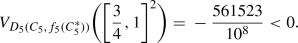
Define the function $f:[0,1]\rightarrow [0,1]$ by and observe that $\smash {f\in {\mathscr {F}}\bigl ([0,1]^{[0,1]}\bigr )}$. For $C=D=\Pi$ we obtain the copula given by

The copula is not absolutely continuous, and the curve $2x+2y-2xy= 1$ has positive mass.

Putting $g= 2-f$, i.e., for each $x\in [0,1]$, we obtain the function given by

Clearly, satisfies the boundary conditions of copulas but we have

i.e., is not a copula. Note that is a proper quasi-copula with a negative mass on the curve $2x+2y-2xy=1$.

6 Concluding remarks

We have introduced and discussed a rather general construction for binary copulas, generalizing several previous approaches. To be precise, we have considered an outer copula $D:[0,1]^2\rightarrow [0,1]$ and a transformation function $f:[0,1]\rightarrow [0,1]$ and provided sufficient (and in some distinguished cases also necessary) conditions for them such that the composite $D(C,f(C^*)):[0,1]^2\rightarrow [0,1]$ is a copula for each inner copula $C:[0,1]^2\rightarrow [0,1]$. This result extends some scenarios considered previously, dealing with composite functions of the form $D(C,C^*)$ (i.e, where f equals the identity function [35]) and $\Pi (C,f(C^*))$ (i.e., where the outer copula D coincides with the product copula [48]).

Moreover, we have shown that, in particular cases, it is possible to leave the unit interval $[0,1]$ (as far as the range of f is concerned), in which case a binary function should replace the outer copula D. This was exemplified in the case when F equals the product on and the inner copula C coincides with $\Pi$.

In this way, for affine transformation functions, the family $\smash {\bigl ({C^{\mathbf {FGM}}_{\theta }}\bigr ){}_{\theta \in [{-1,1}]}}$ of Farlie–Gumbel–Morgenstern copulas can be recovered. Alternatively, the subfamily $\smash {\bigl ({C^{\mathbf {FGM}}_{\theta }}\bigr ){}_{\theta \in [{-1,0}]}}$ can be directly constructed using (3.1) and Theorem 3.5, and for each $\theta \in [0,1]$ the copula $\smash {{C^{\mathbf {FGM}}_{\theta }}}$ can be obtained by flipping $\smash {{C^{\mathbf {FGM}}_{-\theta }}}$ [12, 57].

In a similar way fix W as outer and $\Pi$ as inner copula. Then, for each $\lambda \in [{-1,0}]$ and for the affine function $f_{1+\lambda }:[0,1]\rightarrow [0,1]$ given in (3.30) we get (as in Example 3.11 (ii)) the copula $\smash {K_{\lambda }^{W,\Pi } \!= W(\Pi ,f_{1+\lambda }(\Pi ^*))}$ given by

in particular $\smash {K_{-1}^{W,\Pi }\!=W}$ and $\smash {K_{0}^{W,\Pi }\!=\Pi }$. Putting $\smash {K_{\lambda }^{W,\Pi }\!=\bigl (K_{-\lambda }^{W,\Pi }\bigr ){}^-}$ for $\lambda \in \big ]0,1\big ]$, we get and, in particular, $\smash {K_{1}^{W,\Pi }\!=M}$. Then the family of copulas $\smash {\bigl (K_{\lambda }^{W,\Pi }\bigr ){}_{\lambda \in [{-1,1}]}}$ is comprehensive [57] (i.e., it contains all three basic copulas W, $\Pi$ and M) and continuous and strictly increasing with respect to the parameter $\lambda$.

More generally, the same procedure can be applied to some outer copula D (which is ultramodular and Schur concave on $\Delta$), to all affine functions $f_{\lambda }:[0,1]\rightarrow [0,1]$ with $\lambda \in [{-1,0}]$ as given by (3.30), and to an arbitrary inner copula C. Writing briefly $\smash {K_{\lambda }^{D,C}\!=D(C,f_{\lambda }(C^*))}$ we obtain a monotone non-decreasing parametric family $\smash {(K_{\lambda }^{D,C})_{\lambda \in [{-1,0}]}}$ of copulas with $\smash {K_{0}^{D,C}=C}$. If we denote, for each $\lambda \in \big ]0,1\big ]$, the flipped copula of $\smash {K_{-\lambda }^{D,C}}$ by $\smash {K_{\lambda }^{D,C}}$, we get a parametric family of copulas $\bigl (\smash {K_{\lambda }^{D,C}}\bigr ){}_{\lambda \in [{-1,1}]}$. If, in addition, the inner copula C is invariant with respect to flipping (i.e., if $C^-=C$) then $\bigl (\smash {K_{\lambda }^{D,C}}\bigr ){}_{\lambda \in [{-1,1}]}$ is a monotone non-decreasing family of copulas which is non-trivial (i.e., non-constant) whenever $D\ne M$ and which is continuous with respect to the parameter $\lambda$. Clearly, the family $\bigl (\smash {K_{\lambda }^{D,C}}\bigr ){}_{\lambda \in [{-1,1}]}$ can be seen as a generalization of the family of Farlie–Gumbel–Morgenstern copulas: we have $\smash {K_{\lambda }^{\Pi ,\Pi }\!={C^{\mathbf {FGM}}_{\lambda }}}$ for each $\lambda \in [{-1,1}]$.

As already stressed, the class of functions $\smash {{\mathscr {F}}\bigl ([0,1]^{[0,1]}\bigr )}$ allows us to construct copulas based on an outer copula D (being ultramodular and Schur concave on $\Delta$) and on an arbitrary inner copula C. As an interesting problem for further research one can fix an appropriate outer copula D and look for all functions f such that $D(C,f(C^*))$ is a copula for each inner copula C. Similarly, one can fix the copulas D and C and search for feasible functions f.

References

Alsina, C., Frank, M.J., Schweizer, B.: Associative Functions. World Scientific, Hackensack (2006)
Alsina, C., Nelsen, R.B., Schweizer, B.: On the characterization of a class of binary operations on distribution functions. Statist. Probab. Lett. 17(2), 85–89 (1993)
Aumann, R.J., Shapley, L.S.: Values of Non-Atomic Games. Princeton University Press, Princeton (1974)
Barlow, R.E., Spizzichino, F.: Schur-concave survival functions and survival analysis. J. Comput. Appl. Math. 46(3), 437–447 (1993)
Beccacece, F., Borgonovo, E.: Functional ANOVA, ultramodularity and monotonicity: Applications in multiattribute utility theory. European J. Oper. Res. 210(2), 326–335 (2011)
Capéraà, Ph., Genest, Chr.: Spearman’s \(\rho \) is larger than Kendall’s \(\tau \) for positively dependent random variables. J. Nonparametr. Stat. 2(2), 183–194 (1993)
Cherubini, U., Luciano, E., Vecchiato, W.: Copula Methods in Finance. Wiley, Chichester (2004)
Cuadras, C.M.: Constructing copula functions with weighted geometric means. J. Statist. Plann. Inference 139(11), 3766–3772 (2009)
De Baets, B.: Similarity of fuzzy sets and dominance of random variables: a quest for transitivity. In: Della Riccia, G., et al. (eds.) Preferences and Similarities. CISM International Centre for Mechanical Sciences, vol. 504, pp. 1–22. Springer, Wien (2008)
De Baets, B.: Quasi-copulas: a bridge between fuzzy set theory and probability theory. In: Huynh, V.N., et al. (eds.) Integrated Uncertainty Management and Applications. Advances in Intelligent and Soft Computing, vol. 68, p. 55. Springer, Berlin (2010)
De Baets, B., De Meyer, H.: Orthogonal grid constructions of copulas. IEEE Trans. Fuzzy Systems 15(6), 1053–1062 (2007)
De Baets, B., De Meyer, H., Kalická, J., Mesiar, R.: Flipping and cyclic shifting of binary aggregation functions. Fuzzy Sets and Systems 160(6), 752–765 (2009)
Díaz, S., De Baets, B., Montes, S.: General results on the decomposition of transitive fuzzy relations. Fuzzy Optim. Decis. Mak. 9(1), 1–29 (2010)
Dolati, A., Úbeda-Flores, M.: Constructing copulas by means of pairs of order statistics. Kybernetika (Prague) 45(6), 992–1002 (2009)
Durante, F.: A new class of symmetric bivariate copulas. J. Nonparametr. Stat. 18(7–8), 499–510 (2006)
Durante, F.: New Results on Copulas and Related Concepts. Ph.D. thesis, Università degli Studi di Lecce (2006)
Durante, F.: A new family of symmetric bivariate copulas. C. R. Math. Acad. Sci. Paris 344(3), 195–198 (2007)
Durante, F., Fernández-Sánchez, J., Sempi, C.: Sklar’s theorem obtained via regularization techniques. Nonlinear Anal. 75(2), 769–774 (2012)
Durante, F., Jaworski, P.: A new characterization of bivariate copulas. Comm. Statist. Theory Methods 39(16), 2901–2912 (2010)
Durante, F., Jaworski, P.: Spatial contagion between financial markets: a copula-based approach. Appl. Stoch. Models Bus. Ind. 26(5), 551–564 (2010)
Durante, F., Kolesárová, A., Mesiar, R., Sempi, C.: Semilinear copulas. Fuzzy Sets and Systems 159(1), 63–76 (2008)
Durante, F., Saminger-Platz, S., Sarkoci, P.: On representations of \(2\)-increasing binary aggregation functions. Inform. Sci. 178(23), 4534–4541 (2008)
Durante, F., Saminger-Platz, S., Sarkoci, P.: Rectangular patchwork for bivariate copulas and tail dependence. Comm. Statist. Theory Methods 38(13–15), 2515–2527 (2009)
Durante, F., Sempi, C.: Copulæ and Schur-concavity. Int. Math. J. 3(9), 893–905 (2003)
Durante, F., Sempi, C.: Principles of Copula Theory. CRC Press, Boca Raton (2015)
Genest, C., Quesada Molina, J.J., Rodríguez Lallena, J.A., Sempi, C.: A characterization of quasi-copulas. J. Multivariate Anal. 69(2), 193–205 (1999)
Goncalves, M., Kolev, N., Fabris, A.: Bounds for distorted risk measures. Econ. Qual. Control 23(2), 243–255 (2008)
Gong, W.-M., Sun, H., Chu, Y.-M.: The Schur convexity for the generalized Muirhead mean. J. Math. Inequal. 8(4), 855–862 (2014)
Grabisch, M., Marichal, J.L., Mesiar, R., Pap, E.: Aggregation Functions. Encyclopedia of Mathematics and Its Applications, vol. 127. Cambridge University Press, Cambridge (2009)
Hájek, P., Mesiar, R.: On copulas, quasicopulas and fuzzy logic. Soft Comput. 12(12), 1239–1243 (2008)
Hürlimann, W.: A comprehensive extension of the FGM copula. Statist. Papers 58(2), 373–392 (2017)
Joe, H.: Multivariate Models and Dependence Concepts. Monographs on Statistics and Applied Probability, vol. 73. Chapman & Hall, London (1997)
Joe, H.: Dependence Modeling with Copulas. Monographs on Statistics and Applied Probability, vol. 134. CRC Press, Boca Raton (2015)
Khoudraji, A.: Contributions à l’étude des copules et à la modélisation des valeurs extrêmes bivariées. Ph.D. thesis, Université Laval, Québec (1995)
Klement, E.P., Kolesárová, A., Mesiar, R., Saminger-Platz, S.: On the role of ultramodularity and Schur concavity in the construction of binary copulas. J. Math. Inequal. 11(2), 361–381 (2017)
Klement, E.P., Kolesárová, A., Mesiar, R., Sempi, C.: Copulas constructed from horizontal sections. Comm. Statist. Theory Methods 36(13–16), 2901–2911 (2007)
Klement, E.P., Kolesárová, A., Mesiar, R., Stupňanová, A.: Lipschitz continuity of discrete universal integrals based on copulas. Internat. J. Uncertain. Fuzziness Knowledge-Based Systems 18(1), 39–52 (2010)
Klement, E.P., Manzi, M., Mesiar, R.: Ultramodular aggregation functions. Inform. Sci. 181(19), 4101–4111 (2011)
Klement, E.P., Manzi, M., Mesiar, R.: Ultramodularity and copulas. Rocky Mountain J. Math. 44(1), 189–202 (2014)
Klement, E.P., Mesiar, R., Pap, E.: Triangular Norms. Trends in Logic—Studia Logica Library, vol. 8. Kluwer, Dordrecht (2000)
Klement, E.P., Mesiar, R., Pap, E.: A universal integral as common frame for Choquet and Sugeno integral. IEEE Trans. Fuzzy Systems 18(1), 178–187 (2010)
Klement, E.P., Mesiar, R., Spizzichino, F., Stupňanová, A.: Universal integrals based on copulas. Fuzzy Optim. Decis. Mak. 13(3), 273–286 (2014)
Kolesárová, A.: \(1\)-Lipschitz aggregation operators and quasi-copulas. Kybernetika (Prague) 39(5), 615–629 (2003)
Kolesárová, A., Mesiar, R., Kalická, J.: On a new construction of \(1\)-Lipschitz aggregation functions, quasi-copulas and copulas. Fuzzy Sets and Systems 226, 19–31 (2013)
Li, D.-M., Shi, H.-N.: Schur convexity and Schur-geometrically concavity of generalized exponent mean. J. Math. Inequal. 3(2), 217–225 (2009)
Liebscher, E.: Construction of asymmetric multivariate copulas. J. Multivariate Anal. 99(10), 2234–2250 (2008)
Ling, C.: Representation of associative functions. Publ. Math. Debrecen 12, 189–212 (1965)
Manstavičius, M., Bagdonas, G.: A class of bivariate copula mappings. Fuzzy Sets and Systems 354, 48–62 (2019)
Marinacci, M., Montrucchio, L.: Ultramodular functions. Math. Oper. Res. 30(2), 311–332 (2005)
Marinacci, M., Montrucchio, L.: On concavity and supermodularity. J. Math. Anal. Appl. 344(2), 642–654 (2008)
Marshall, A.W., Olkin, I.: Majorization in multivariate distributions. Ann. Statist. 2, 1189–1200 (1974)
Marshall, A.W., Olkin, I., Arnold, B.C.: Inequalities: Theory of Majorization and Its Applications. Springer Series in Statistics, 2nd edn. Springer, New York (2011)
Mesiar, R., Jágr, V., Juráňová, M., Komorníková, M.: Univariate conditioning of copulas. Kybernetika (Prague) 44(6), 807–816 (2008)
Mesiar, R., Szolgay, J.: \(W\)-ordinal sums of copulas and quasi-copulas. In: Proceedings MAGIA & UWPM 2004, pp. 78–83. Slovak University of Technology, Bratislava (2004)
Moynihan, R.: On \(\tau _T\) semigroups of probability distribution functions II. Aequationes Math. 17(1), 19–40 (1978)
Müller, A., Scarsini, M.: Stochastic comparison of random vectors with a common copula. Math. Oper. Res. 26(4), 723–740 (2001)
Nelsen, R.B.: An Introduction to Copulas. Springer Series in Statistics, 2nd edn. Springer, New York (2006)
Nevius, S.E., Proschan, F., Sethuraman, J.: Schur functions in statistics. II. Stochastic majorization. Ann. Statist. 5(2), 263–273 (1977)
Proschan, F., Sethuraman, J.: Schur functions in statistics. I The preservation theorem. Ann. Statist. 5(2), 256–262 (1977)
Roberts, A.W., Varberg, D.E.: Convex Functions. Pure and Applied Mathematics, vol. 57. Academic Press, New York (1973)
Rockafellar, R.T.: Convex Analysis. Princeton Mathematical Series, vol. 28. Princeton University Press, Princeton (1970)
Rovenţa, I.: A note on Schur-concave functions. J. Inequal. Appl. 2012, 159 (2012)
Sainio, E., Turunen, E., Mesiar, R.: A characterization of fuzzy implications generated by generalized quantifiers. Fuzzy Sets and Systems 159(4), 491–499 (2008)
Saminger-Platz, S., Dibala, M., Klement, E.P., Mesiar, R.: Ordinal sums of binary conjunctive operations based on the product. Publ. Math. Debrecen 91(1–2), 63–80 (2017)
Schur, I.: Über eine Klasse von Mittelbildungen mit Anwendungen auf die Determinantentheorie. Sitzungsber. Berl. Math. Ges. 22, 9–20 (1923)
Schweizer, B., Sklar, A.: Associative functions and abstract semigroups. Publ. Math. Debrecen 10, 69–81 (1963)
Schweizer, B., Sklar, A.: Probabilistic Metric Spaces. North-Holland Series in Probability and Applied Mathematics. North-Holland, New York (1983)
Shaked, M., Shanthikumar, J.G.: Stochastic Orders. Springer Series in Statistics. Springer, New York (2007)
Shi, H.-N.: Schur-convex functions related to Hadamard-type inequalities. J. Math. Inequal. 1(1), 127–136 (2007)
Shi, H.-N., Zhang, J.: Schur-convexity, Schur geometric and Schur harmonic convexities of dual form of a class symmetric functions. J. Math. Inequal. 8(2), 349–358 (2014)
Shi, H.-N., Zhang, J., Gu, C.: New proofs of Schur-concavity for a class of symmetric functions. J. Inequal. Appl. 2012, # 12 (2012)
Siburg, K.F., Stoimenov, P.A.: Gluing copulas. Comm. Statist. Theory Methods 37(18–20), 3124–3134 (2008)
Sklar, A.: Fonctions de répartition à \(n\) dimensions et leurs marges. Publ. Inst. Statist. Univ. Paris 8, 229–231 (1959)
Sugeno, M.: Theory of Fuzzy Integrals and Its Applications. Ph.D. thesis, Tokyo Institute of Technology (1974)
Weber, S.: A general concept of fuzzy connectives, negations and implications based on \(t\)-norms and \(t\)-conorms. Fuzzy Sets and Systems 11(2), 115–134 (1983)
Wright, E.M.: An inequality for convex functions. Amer. Math. Monthly 61, 620–622 (1954)
Yager, R.R.: Joint cumulative distribution functions for Dempster–Shafer belief structures using copulas. Fuzzy Optim. Decis. Mak. 12(4), 393–414 (2013)
Acknowledgements
Open access funding provided by Johannes Kepler University Linz. The authors would like to thank the two anonymous referees for their careful work and their thoughtful suggestions which helped to correct some errors in an earlier version of the paper.
Author information
Authors and Affiliations
Corresponding author
Additional information
Publisher's Note
Springer Nature remains neutral with regard to jurisdictional claims in published maps and institutional affiliations.
The support by the “Technologie-Transfer-Förderung” of the Upper Austrian Government (Wi-2014-200710/13-Kx/Kai) is gratefully acknowledged, as well as the support by the Slovak Grants APVV-14-0013, VEGA 1/0614/18 and VEGA 1/0891/17.
Rights and permissions
Open Access This article is distributed under the terms of the Creative Commons Attribution 4.0 International License (http://creativecommons.org/licenses/by/4.0/), which permits unrestricted use, distribution, and reproduction in any medium, provided you give appropriate credit to the original author(s) and the source, provide a link to the Creative Commons license, and indicate if changes were made.
About this article
Cite this article
Saminger-Platz, S., Kolesárová, A., Mesiar, R. et al. The key role of convexity in some copula constructions. European Journal of Mathematics 6, 533–560 (2020). https://doi.org/10.1007/s40879-019-00346-3
Received:
Revised:
Accepted:
Published:
Issue Date:
DOI: https://doi.org/10.1007/s40879-019-00346-3