Polynomial approach to explicit formulae for generalized binomial coefficients

Abstract

We extend the polynomial approach to the hook length formula proposed in Károlyi et al. Adv Math 277:252–282 (2015) to several other problems of the same type, including the number of paths formula in the Young graph of strict partitions.

The multivariate polynomial interpolation, or, in other words, the explicit form of Alon’s Combinatorial Nullstellensatz [9, 13], recently proved to be powerful in proving polynomial identities: in [9] it was used for the direct short proof of Dyson’s conjecture, later generalized in [10] for the equally short proof of the q-version of Dyson’s conjecture, then after additional combinatorial work it allowed to prove identities of Morris, Aomoto, Forrester (the last was open), their common generalizations, both in classical and q-versions.

Here we outline how this method works in classical theory of symmetric functions, “self-proving” polynomial identities corresponding to the counting paths in the Young graph and “strict Young graph”, or, in other words, counting dimensions of linear and projective representations of symmetric groups.

The interpolation-based approach to symmetric functions has been earlier developed by Olshanski, Borodin, Okounkov, Vershik, Regev [5, 14–16] and others. It may sound speculatively, but according to author’s opinion, the novelty of my/author’s approach consists in considering arbitrary polynomials (rather antisymmetric, than symmetric) as functions of usual points and applying general facts about general (not symmetric) polynomials instead of considering “symmetric functions as functions of partitions” (formulation from [5]).

We start with a general framework of paths in graded graphs.

1 Graded graphs

Let G be a $\mathbb {Z}$-graded countable directed graph with the vertex set , directed edges $(u,v)\in E(G)$ joining vertices of the consecutive levels $u\in V_i$ and $v\in V_{i+1}$ for some integer i. In what follows both indegrees and outdegrees of all vertices are bounded. This implies that the number $P_{G}(v,u)$ of directed paths from v to u is finite for any two fixed vertices v, u. This number is known as the generalized binomial coefficient (usual binomial coefficient appears for the Pascal triangle).

Fix a positive integer k. Our examples are induced subgraphs of the lattice $\mathbb {Z}^k$. Vertices are graded by the sum of coordinates, edges correspond to increasing of any coordinate by 1. That is, indegree of any vertex equals its outdegree and equals k. It is convenient to identify the vertex set V with the monomials , $(c_1,\dots ,c_k)\in \mathbb {Z}^k$. Then any edge corresponds to multiplying of monomial by some variable $x_i$. Finite linear combinations of elements of V (with, say, rational coefficients, it is not essential hereafter) form a ring of Laurent polynomials in variables $x_1,\dots ,x_k$. Not necessary finite linear combinations form a -module which we denote by $\Phi$. For monomial $v\in V$ and $\varphi \in \Phi$ we denote by the coefficient of v in the series $\varphi$.

Define the minimum of two monomials $u=\prod x_i^{a_i}$ and $v=\prod x_i^{b_i}$ as . If we say that the monomial v majorates u.

Now we describe three examples of graded graphs for which explicit formulae for generalized binomial coefficients are known.

• Multidimensional Pascal graph $\mathcal {P}_k$. This is a subgraph of $\mathbb {Z}^k$ formed by the vectors with integral non-negative coordinates (or, in the monomial language, by monomials having all variables in non-negative power). For $k=2$ this graph is isomorphic to the Pascal triangle.

• Restricted Young graph $\mathcal {Y}_k$. This is a subgraph of the Pascal graph formed by vectors $(c_1,\dots ,c_k)$ with strictly increasing non-negative coordinates, $0\leqslant c_1<c_2<\cdots <c_k$. The vertices of $\mathcal {Y}_k$ may be identified with the Young diagrams having at most k rows (to any vertex $(c_1,\dots ,c_k)$ of $\mathcal {Y}_k$ we assign a Young diagram with rows (to any vertex $(c_1,\dots ,c_k)$ of $\mathcal {Y}_k$ we assign a Young diagram with lengths of rows $c_1\leqslant c_2-1\leqslant \cdots \leqslant c_k-(k-1)$). Edges correspond to addition of boxes. The usual Young graph has all Young diagrams as vertices, but when we count number of paths between two diagrams we may always restrict ourselves to $\mathcal {Y}_k$ with large enough k.

• Graph of strict partitions $\mathcal {SY}_k$. This is a subgraph of the Pascal graph formed by vectors $(c_1,\dots ,c_k)$ with non-strictly increasing non-negative coordinates $0\leqslant c_1\leqslant c_2\leqslant \cdots \leqslant c_k$ satisfying the following condition: if $c_i=c_{j}$ for $i\ne j$, then $c_i=0$. To any vertex $(c_1,\dots ,c_k)$ we may assign a Young diagram with lengths of rows $c_1,\dots ,c_k$. So, this diagram has at most k (non-empty) rows and they have distinct lengths.

The following general straightforward fact connects generalized binomial coefficients for subgraphs of $\mathbb {Z}^k$ with coefficients of polynomials or power series.

Theorem 1.1

Let G be a subgraph of $\mathbb {Z}^k$, monomials $u,v\in V(G)$ be two vertices of G, $\deg u\geqslant \deg v$. Assume that $\varphi \in \Phi$ is a series satisfying the following conditions:

• (i) ;

• (ii) if $v'\in V(G)$ and $\deg v=\deg v'$, then ;

• (iii) if $w\notin V(G)$, but $x_iw\in V(G)$ for some $x_i$, then .

Then the number of paths from v to u equals

(1)

Proof

Induction on $\deg u$. The base $\deg u=\deg v$ follows from (i) and (ii). Denote $m=\deg u-\deg v$ and assume that the statement is proved for all vertices of degree less than $m+\deg v$. Let $(u_i,u)$, $i=1,\dots ,s$, be all edges of the graph G coming to u. Clearly $s\leqslant k$ and without loss of generality $u=x_iu_i$ for $i=1,\dots ,s$. Also note that for $s<i\leqslant k$ we have by property (iii). Thus

as desired. $\square$

Remark 1.2

In other words, both parts of (1) are fundamental solutions of the Laplace equation on the part of our graph starting from the level of v.

Theorem 1.1 leads to a natural question: for which labeled graphs (G, u) there exists a function $\varphi$ such that conditions (i)–(iii) are satisfied? We do not know a full answer. The following statement is at least general enough to cover all examples of this paper.

Theorem 1.3

Assume that $V\subset \mathbb {Z}^k$, G is the induced subgraph of $\mathcal P_k$ with vertex set $V=V(G)$ and it satisfies the following two conditions:

• (i) (minimum-closed set) if $u,w\in V$, then also .

• (ii) (coordinate convexity) if $u,w\in V$, $w=ux_i^m$ for some index i and positive integer m, then also $ux_i^s\in V$ for all $0\leqslant s\leqslant m$.

Then for any $v\in V$ there exists a function $\varphi$ satisfying conditions of Theorem 1.1.

Proof

Call a monomial $u\in \mathbb {Z}^k$ special if either $u\in V$, $\deg u=\deg v$ (in particular, v itself is special), or $\deg u\geqslant \deg v$, $u\notin V$, $x_iu\in V$ for some variable $x_i$. It suffices to prove that there exists a function $\varphi$ homogeneous of degree $\deg v$ with any prescribed values of for all special u. This is a linear system on coefficients of $\varphi$.

By replacing V with $v^{-1}V$ we may suppose that $v=1$. For any special monomial u define its son S(u) as follows: if $\deg u=0$, then $S(u)=0$, if $u\notin V$, $x_iu\in V$, then $S(u)=x_i^{-\deg u} u$ (if different indexes i satisfy $x_iu\in V$, choose any).

If $u\ne w$ are two special monomials and w majorates S(u), then $\deg w>\deg u$. Indeed, assume that on the contrary $\deg w\leqslant \deg u$. First, if $\deg u=0$, then $\deg w=0$ and $w=S(u)=u$, a contradiction. Thus $d=\deg u>0$, we may suppose that $x_1u\in V$, $S(u)=x_1^{-d} u$. Denote , $a_i\geqslant 0$, $d\geqslant a_1+\cdots +a_k$, and either $w\in V$ or $x_iw\in V$ for some i. Since $w\ne u$, we have $d>a_1$. Denote if $x_iw\in V$, and if $w\in V$. Then $u_0=x_1^{a_1-d+\varepsilon }u$, where , and $u_0\in V$ since V is a minimum-closed set. The coordinate convexity implies that if both $u_0,x_1u$ belong to V, so does u. A contradiction.

Now we start to solve our linear system for coefficients of $\varphi$. For any special monomial u we have a linear relation on the monomials of degree 0 majorated by u. Between them there is a monomial S(u), and it does not appear in relations corresponding to special monomials $w\ne u$ with $\deg w\leqslant \deg u$. It allows to fix coefficients of $\varphi$ in the appropriate order (by increasing the degree of u) and fulfil all our relations. $\square$

2 Observation on polynomials

Recall the Combinatorial Nullstellensatz of Alon [1].

Theorem 2.1

(Combinatorial Nullstellensatz) Let K be a field and $A_i$, $i=1,\dots ,k$, be non-empty subsets of K, $|A_i|=d_i+1$. Let be a polynomial of degree at most $d_1+\cdots +d_k$ such that $f(c_1,\dots ,c_k)=0$ for all points . Then

For verifying polynomial identities which allow to calculate coefficients we use the following observation in the spirit of the Combinatorial Nullstellensatz.

Let K be a field and , $i=1,\dots ,k$, be its subsets of size $|A_i|=n+1$.

Observation 2.2

A polynomial of degree at most n is uniquely determined by its values on the combinatorial simplex

Proof

The number of points in $\Delta$ equals exactly the dimension of the space of polynomials with degree at most n in k variables. Hence it suffices to check either existence or uniqueness of the polynomial with degree at most n and with prescribed values on $\Delta$. Both tasks are easy as we may see:

Existence. Induction on n. The base $n=0$ is clear. Assume that $n>1$ and for the simplex $\Delta '$, which corresponds to the inequality $\sum t_i\leqslant n-1$, there exists a polynomial $f(x_1,\dots ,x_k)$ with degree at most $n-1$ and with prescribed values on $\Delta '$. For any point $A(t_1,\dots ,t_k)$ with $\sum t_i=n$ we have a polynomial

vanishing on all points of $\Delta$ but $A(t_1,\dots ,t_k)$. The appropriate linear combination of f(x) and such polynomials gives a polynomial with the prescribed values on $\Delta$ (and degree at most n).

Uniqueness. It suffices to prove that the polynomial $f(x_1,\dots ,x_k)$ with degree at most n, which vanishes on $\Delta$, identically equals 0. Assume the contrary. Let be a highest degree term in f. The set $\Delta$ contains the product , where , $|B_i|=t_i+1$. By the Combinatorial Nullstellensatz, f cannot vanish on $\prod B_i$. A contradiction. $\square$

For we get the standard simplex

It is the main partial case for us. In the theory of q-identities its q-analogue, which corresponds to the set , plays an analogous role.

We use notations ${x}^{\underline{n}}=x(x-1)\cdots (x-n+1)$ and $\left( {\begin{array}{c}x\\ n\end{array}}\right) ={x}^{\underline{n}}/n!$.

Remark 2.3

Some other notations, including are used for falling factorials. I/author prefer the Capelli–Toscano notation, popularized by Knuth, see his arguments in [12]. The author finds it quite intuitive, particularly in the context of this paper.

The following particular case of interpolation on $\Delta _k^n$ appears to be useful.

Lemma 2.4

If , $\deg f\leqslant n$ and f vanishes on $\Delta _k^{n-1}$, then

Proof

It suffices to check the equality for values on $\Delta _k^n$. Both parts vanish on $\Delta _k^{n-1}$. If $(x_1,\dots ,x_k)$ is a point on , i.e. $\sum x_i=n$, then all summands on the right vanish except (possibly) the summand with $c_i=x_i$ for all i, and its value just equals $f(c_1,\dots ,c_k)=f(x_1,\dots ,x_k)$, i.e. the value of LHS at the same point, as desired. $\square$

We start our series of applications of Observation 2.2 along with the multinomial version of the Chu–Vandermonde identity.

2.1 Example: Chu–Vandermonde identity and multinomial coefficient

(2)

This immediately follows from Lemma 2.4.

Identity (2) has the following form in falling factorials:

(3)

Taking only the leading terms in both sides we get the Multinomial Theorem, i.e.

(4)

Returning back to graded graphs, for the multidimensional Pascal graph $\mathcal {P}_k$ we get the following formula for the number of paths from the origin 1 to any vertex $v=\prod x_i^{m_i}$, $m_i\geqslant 0$, $n=\sum m_i=\deg v$:

This immediately follows from Theorem 1.1 for $\varphi =1$ and identity (4).

3 Hook length formula

We start with a polynomial identity which is in a sense similar to the Chu–Vandermonde identity (3).

Theorem 3.1

Proof

By Lemma 2.4, it suffices to check that LHS vanishes on $\Delta _k^{n+k(k-1)/2-1}$. Let $x_i$ be non-negative integers and $\sum x_i<n+k(k-1)/2$. If $\sum x_i<k(k-1)/2$ then some factor $x_i-x_j$ vanishes, otherwise $y=\sum x_i-k(k-1)/2$ is non-negative and $y<n$, hence .$\square$

As in the Chu–Vandermonde case, we may take only the leading terms and get the identity

$$\begin{aligned} {\begin{matrix} \prod _{i<j}(x_j-x_i)&{}(x_1+\cdots +x_k)^n\\ &{}=\!\!\!\!\!\sum _{n_1+\cdots +n_k=n+k(k-1)/2}\frac{n!}{\prod n_i!} \prod _{i<j}(n_j-n_i)\cdot \prod {x_i}^{n_i}\!. \end{matrix}} \end{aligned}$$

(5)

Being divided by $\prod _{i<j} (x_j-x_i)$, this becomes a well-known expansion

$$\begin{aligned} (x_1+x_2+\cdots )^n=\sum _{\lambda \vdash n} \dim \lambda \cdot s_{\lambda } \end{aligned}$$

for the Schur symmetric functions (combined with the Frobenius formula for dimensions).

Corollary 3.2

(Frobenius dimension formula) For any vertex , $\sum n_i=n+k(k-1)/2$, of the Young graph $\mathcal {Y}_k$ the number of paths to this vertex from $v_0=(0,1,\dots ,k-1)$ equals

(6)

Proof

Take $\varphi =\prod _{i<j}(x_j-x_i)$ and apply Theorem 1.1. Conditions (i) and (ii) follow from (5) with $n=0$ (actually, this is just the Vandermonde determinant formula). For checking (iii), note that such $w=\prod x_i^{n_i}$ satisfies either $n_i<0$ for some i or $n_i=n_j$ for some i, j. In both cases (5) yields that the corresponding coefficient vanishes. $\square$

Note that our proof of (6) does not use the Multinomial Theorem, but is proved in the same way and the proof is almost equally short. Identity (5) appears also in the important for the development of the polynomial method paper [2], where it is used for appropriate application of the Combinatorial Nullstellensatz, while we show how it may be proved by the (explicit version of) Combinatorial Nullstellensatz.

In the rest part of this section we explain the relation of (6) with hook lengths of the Young diagram, this is mostly for the sake of completeness.

Recall that the graph $\mathcal {Y}_k$ may be viewed as the graph of Young diagrams having at most k rows. For a vertex $v\in \mathcal {Y}_k$, , the corresponding diagram $\lambda (v)$ has k (possibly empty) rows with lengths $n_1\leqslant n_2-1\leqslant \cdots \leqslant n_k-(k-1)$. Edges of the graph $\mathcal {Y}_k$ correspond to adding boxes, and paths correspond to the skew standard Young tableaux: for any path with, say m edges, put numbers $1,2,\dots ,m$ in the corresponding adding boxes. In this language, expression (6) counts the number of standard Young tableaux of the shape $\lambda (v)$. Assuming $n_1>0$ (i.e. the number of rows equals k), we may interpret parameters $n_1,\dots ,n_k$ as hook lengths of k boxes in the first column. Recall that (now specify that the largest column in the Young diagram is the leftmost and the largest row is the lowest) a hook of a box X in the Young diagram is a union of X; all boxes in the same column which are higher than X; all boxes in the same row which are on the right to X.

Claim

In the above notations the product of hook lengths of all boxes in the Young diagram $\lambda (v)$ equals

Proof

Assume that boxes a, b of the Young diagram lie in the same row and a, c in the same column. Let d be a box such that abdc is a rectangle. If d belongs to the diagram then $h(a)<h(b)+h(c)$, otherwise $h(a)>h(b)+h(c)$. Hence we always have the inequality $h(a)\ne h(b)+h(c)$. Now $n_1,\dots ,n_k$ are hook lengths of boxes in the first column. In the i-th row there are boxes, and their hook lengths are distinct numbers from 1 to $n_i$, with $i-1$ values excluded, and those excluded values are $n_i-n_1, n_i-n_2, \dots , n_i-n_{i-1}$, by the inequality. It remains to multiply over $i=1,2,\dots ,k$. $\square$

The above claim allows to formulate Corollary 3.2 in the form of the hook length formula [6].

Theorem 3.3

(hook length formula) The number of the standard Young tableaux of a given shape $\lambda$ with n boxes equals $n!/\prod _{\square } h(\square )$, where the product is taken over all boxes of $\lambda$.

Remark 3.4

As the referee pointed out, Theorem 3.1 may be derived from the formalism of [5] combined with the Frobenius dimension formula.

4 Skew Young tableaux

Here we get generalizations of Theorem 3.1, corresponding to counting paths between two arbitrary vertices of $\mathcal {Y}_k$ (i.e. the number of skew Young tableaux of a given shape).

The role of the Vandermonde determinant is played by alternating determinants

The following identity specializes to Theorem 3.1 for $m_i=i-1$, $i=1,2,\dots ,k$.

Theorem 4.1

If $m_1<\cdots <m_k$ are distinct non-negative integers, $m=\sum m_i$, then

Proof

Due to Lemma 2.4, it suffices to check that LHS vanishes on $\Delta _k^{n+m-1}$. Fix a point $(x_1,\dots ,x_k)\in \Delta _k^{n-1}$. Let $y_1\leqslant \dots \leqslant y_k$ be the increasing permutation of $x_i'$. If $y_i<m_i$ for some i, then the matrix is singular as it has minor of zeros, and the matrix is therefore singular too. If $y_i\geqslant m_i$ for all i, then denoting $y=\sum x_i-m=\sum (y_i-m_i)\geqslant 0$ we have $0\leqslant y<n$, hence . $\square$

Taking the leading terms we get the following identity for homogeneous polynomials:

(7)

Corollary 4.2

(skew dimension formula) Let , be two vertices of the Young graph $\mathcal {Y}_k$ such that $n_i\geqslant m_i$ for all $i=1,2,\dots ,k$. Denote $\sum m_i=m$, $\sum n_i=n+m$. Then the number of paths from $v_1$ to $v_2$ equals

Proof

Take $\varphi =a_{m_1,\dots ,m_k}(x_1,\dots ,x_k)$ and apply Theorem 1.1. Conditions (i) and (ii) follow from (7) with $n=0$ (or from expanding the determinant). For checking (iii), note that such $w=\prod x_i^{n_i}$ satisfies either $n_i<0$ for some i or $n_i=n_j$ for some i, j. In both cases (7) yields that the corresponding coefficient vanishes. $\square$

Remark 4.3

This formula for the number of paths between two arbitrary vertices of the Young graph appeared in [15, Theorem 8.1], see also [16]. Recently it appeared in the context of additive combinatorics in [3, Lemma 4], [4].

The value $b_{m_1,\dots ,m_k}(n_1,\dots ,n_k)$ has a combinatorial interpretation following from the Lindström–Gessel–Viennot Lemma: up to a multiple $\prod m_i!$ it is a number of semistandard Young tableaux of a given shape and content. See details in [7].

A.M. Vershik pointed out that similar results are known for the graph of strict diagrams. It also may be included in our framework.

5 Strict diagrams

For counting the number of paths in the graph $\mathcal {SY}_k$ we need series which are not polynomials.

Let $x_1,\dots ,x_k$ be variables (as before). Consider the set $\mathcal {M}$ of rational functions in those variables with denominator . Expand such functions in Laurent series in $x_1,x_2/x_1,x_3/x_2,\dots ,x_k/x_{k-1}$ (i.e., for $i<j$). Define the value of such function at a point $(c_1,\dots ,c_k)$ with non-negative coordinates as follows: if coordinates are positive, just substitute them in the function, if some coordinates vanish, replace them by positive numbers (in such order), and let t tend to . What we actually need is that for $i<j$ the value with $x_i=x_j=0$ equals 0. Each function $f\in \mathcal {M}$ may be expanded as $f=P[f]+Q[f]$, where P[f] is a polynomial in $x_1,\dots ,x_k$, and in Q[f] each term $\prod x_i^{c_i}$ contains at least one variable $x_i$ in a negative power $c_i<0$. We say that P[f] is the polynomial component of f and Q[f] is the antipolynomial component of the function $f(x_1,\dots ,x_k)$.

Lemma 5.1

Define a function $f_n(x_1,\dots ,x_k)\in \mathcal {M}$ by the formula

Then

• (i) its antipolynomial component $Q[f_n]$ vanishes on the standard simplex $\Delta _k^n$,

• (ii) if $c_1,\dots ,c_k$ are integers such that $c_j<0$, $c_i\geqslant 0$ for $i=j+1,\dots ,k$, then $\bigl [\prod x_i^{c_i}\bigr ]f_n=0$.

Proof

We may suppose that $k=2d$ is even (else replace k with $k+1$ and put $x_{k+1}=0$). Consider the following antisymmetric matrix: . Note that its Pfaffian lies in $\mathcal {M}$, it is homogeneous of order 0, it vanishes for $x_i=x_j$ and is singular for . Thus up to a constant multiple (it is not hard to verify that actually up to a sign) it equals . The Pfaffian is an alternating sum of expressions like

where . On the other hand, the Vandermonde identity (2) allows to express the falling factorial as a linear combination of expressions like

Fixing at first the partition into pairs and next the exponents $\alpha _1,\dots ,\alpha _d$, we reduce both claims to the expression

Note that variables are separated here, thus the polynomial component of this product is just the product of polynomial components of the factors. We have

If $\alpha _i\geqslant 1$, the corresponding fraction is a polynomial. If $\alpha _i=0$, we have $\xi _i=x_a$, $\zeta _i=x_b$ for some indexes $a<b$, we use the relation . Substituting $(x_1,\dots ,x_k)\in \Delta _k^n$, we see that if $\xi _i+\zeta _i<\alpha _i$ for some index i, both minuend and the subtrahend take zero value, otherwise $\xi _i=\zeta _i=0$ for all i with $\alpha _i=0$, thus the corresponding factors in the minuend and subtrahend are equal.

For proving (ii), note that we should have $x_j=\xi _s$ for some s, but if $\xi _s$ is taken in negative power, then $\zeta _s=x_{b_s}$ must be taken in positive power and $b_s>j$. $\square$

Modulo this lemma everything is less or more the same as in previous sections.

Theorem 5.2

The polynomial component of the function $f_n(x_1,\dots ,x_k)$ equals

(recall that for $m_i=m_j=0$ is equal to 1).

Proof

Both parts are polynomials of degree at most n, thus it suffices to check that their values at each point $(c_1,\dots ,c_k)\in \Delta _k^n$ are equal. The polynomial component of $f_n(x_1,\dots ,x_k)$ takes the same values on $\Delta _k^n$ as the function $f_n$. Thus, by Lemma 2.4, it suffices to check that $f_n$ vanishes on $\Delta _k^{n-1}$. But already the factor vanishes on $\Delta _k^{n-1}$. $\square$

Corollary 5.3

The coefficient $H(m_1,\dots ,m_k)$ of the Laurent series

$$\begin{aligned} \prod _{1\leqslant i<j\leqslant k} \frac{x_i-x_j}{x_i+x_j} \cdot (x_1+\cdots +x_k)^n \end{aligned}$$

in monomial $\prod x_i^{m_i}$, $m_i\geqslant 0$, equals .

Corollary 5.4

If $u=\prod x_i^{m_i}$ is a vertex of $\mathcal {SY}_k$, $n=\sum m_i$, then the number of paths from the origin to v equals

Proof

Apply Theorem 1.1 to the function . Then the result directly follows from Corollary 5.3, so it suffices to check all conditions of Theorem 1.1. Condition (i) follows from Corollary 5.3 for $n=0$ (or just from common sense). In condition (ii) there is nothing to check since 1 is the unique vertex of $\mathcal {SY}_k$ with degree 0. Let us check condition (iii). Assume that $w=\prod x_i^{c_i}$ is such that $x_iw$ is a vertex of $\mathcal {SY}_k$ but w is not. There are two cases: either all coordinates of w are non-negative and $c_j=c_l>0$ for some j, l, or , $c_j= 0$ for all $j\geqslant i$. In the first case apply Corollary 5.3, in the second case apply statement (ii) of Lemma 5.1. $\square$

6 Skew strict Young tableaux

Here we give an identity corresponding to the formula [8, 17] for the number of paths between any two vertices of the graph $\mathcal {SY}_k$, or, in other words, for the number of strict skew Young tableaux of a given shape.

Let $v=\prod _{i=1}^k x_i^{m_i}$, $m_1>m_2>\cdots >m_{\ell }>m_{\ell +1}=0=\cdots =m_k$, be a vertex of $\mathcal {SY}_k$, $u=\prod x_i^{n_i}$ be another vertex of $\mathcal {SY}_k$ and $n_i\geqslant m_i$ for all i (thus there exists some path from u to v). Denote $m=\sum m_i$, $n=\sum n_i$.

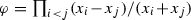
For counting such paths we introduce the following polynomial (Ivanov in [8] attributes it to Okounkov):

Here , where summation is taken over all k! permutations of numbers $1,\dots ,k$. (For concluding that it is indeed a polynomial note that any multiple $x_i-x_j$ in denominator disappears after natural pairing of summands. It is a super-symmetric polynomial, but we do not use this fact.)

Then define the function

The following theorem generalizes results of the previous section.

Theorem 6.1

Denote .

• (i) The antipolynomial component vanishes on the simplex $\Delta _k^n$.

• (ii) The polynomial component of g has the expansion

  

  (8)

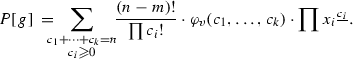
• (iii) The number of paths from $v=\prod x_i^{m_i}$ to $u=\prod x_i^{n_i}$ equals

  $$\begin{aligned} \frac{(n-m)!}{\prod n_i!} \cdot \varphi _v(n_1,\dots ,n_k). \end{aligned}$$

Proof

(i) Fix a permutation $\pi$ and prove the statement for the antipolynomial component of the corresponding summand in the definition of $\varphi _v$. Denote $y_i=x_{\pi _i}$. Note that up to a sign our summand is

We expand as a Pfaffian as explained in the proof of Lemma 5.1 (if $k-\ell$ is odd do the same thing as before: add a vanishing variable; so let $k-\ell =2d$ be even). Expand this Pfaffian, and take a summand like , where .

Expand also by the Chu–Vandermonde identity (2) as a linear combination of terms like

$\sum \alpha _i+\sum \beta _i=n-m$. Thus it suffices to prove that the antipolynomial component of the following product vanishes on $\Delta _k^n$:

The variables are separated, hence the polynomial component of the product is a product of polynomial components. It suffices to verify that whenever $y_i,\xi _i,\zeta _i$ are non-negative integers with sum at most n, the values of and are equal. If $\beta _i\geqslant 1$, the corresponding fraction is a polynomial. If $\beta _i=0$, we have $\xi _i=x_a$, $\zeta _i=x_b$ for some indexes $a<b$, then . Substituting $(x_1,\dots ,x_k)\in \Delta _k^n$, we see that if $y_i<m_i+\alpha _i$ or $\xi _i+\zeta _i<\beta _i$ for some index i, then both products take zero value, otherwise $\xi _i=\zeta _i=0$ for all i with $\beta _i=0$, thus the corresponding fractions (values of the function and its polynomial part) are equal.

Note that as in Lemma 5.1 we may also conclude that if $c_1,\dots ,c_k$ are integers such that $c_j<0$, $c_i\geqslant 0$ for $i=j+1,\dots ,k$, then .

(ii) The values of on $\Delta _k^n$ are the same as values of g. Any summand of the above expansion for g vanishes on $\Delta _k^{n-1}$. Thus it suffices to use Lemma 2.4.

(iii) Apply Theorem 1.1 to the function $\varphi _v$ (or its leasing part, it is a matter of taste). It suffices to check all conditions of Theorem 1.1. Conditions (i) and (ii) follow from the above expansion of g (with $n=0$). There are exactly permutations with $y_i=x_i$, $i=1,\dots ,\ell$, for each of them we get coefficient 1 in the monomial v and coefficient 0 in other monomials of degree m. For other permutations we do not get non-zero coefficients in monomials which are vertices of $\mathcal {SY}_k$. Let us check condition (iii). Assume that $w=\prod x_i^{c_i}$ is such that $x_iw$ is a vertex of $\mathcal {SY}_k$ but w is not. There are two cases: either all coordinates of w are non-negative and $c_j=c_l>0$ for some j, l, or $c_i=-1$, $c_j= 0$ for all $j\geqslant i$. In the first case apply identity (8), in the second case apply the above remark after the proof of part (i) of the theorem. $\square$

7 Concluding remarks

For the sake of convenience we summarize here the list of functions $\varphi$ for which coefficients of $\varphi \bigl (\sum x_i\bigr )^N$ count the number of paths from the vertex v in some graded graph G.

• (a) $\varphi =\prod x_i^{m_i}$, $v=\prod x_i^{m_i}$, G is the multidimensional Pascal graph ${\mathcal P}_k$.

• (b) , $m_1<m_2<\dots <m_k$, $v=\prod x_i^{m_i}$, G is the Young graph ${\mathcal Y}_k$ formed by strictly increasing sequences.

• (c) , v is the origin, $G={\mathcal SY}_k$ is the graph of strict Young diagrams. When v is not the origin, the corresponding function $\varphi _v$ should be multiplied by the Okounkov polynomial, as described in Sect. 6.

We may observe that functions $\varphi$ in examples (b) and (c) vanish on the “boundary” of the corresponding graph considered as a subgraph of ${\mathcal P}_k$. However, we do not know how to guess the function of example (c) without knowing it a priori. Hopefully, the answer to this question may help to generalize this machinery to other graphs.

Another question which has to be answered is how identities with falling factorials are related with asymptotics of dimensions.

References

Alon, N.: Combinatorial Nullstellensatz. Combin. Probab. Comput. 8(1–2), 7–29 (1999)
Alon, N., Nathanson, M.B., Ruzsa, I.: The polynomial method and restricted sums of congruence classes. J. Number Theory 56(2), 404–417 (1996)
Balandraud, É.: An addition theorem and maximal zero-sum free sets in \(\mathbb{Z}/p\mathbb{Z}\). Israel J. Math. 188, 405–429 (2012)
Balandraud, É.: Erratum to: “An addition theorem and maximal zero-sum free sets in \({\mathbb{Z}}/p{\mathbb{Z}}\)”. Israel J. Math. 192(2), 1009–1010 (2012)
Borodin, A., Olshanski, G.: Harmonic functions on multiplicative graphs and interpolation polynomials. Electron. J. Combin. 7, R28 (2000)
Frame, J.S., Robinson, G. de B., Thrall, R.M.: The hook graphs ofthe symmetric groups. Canad. J. Math. 6, 316–324 (1954)
Fulmek, M.: Viewing determinants as nonintersecting lattice paths yields classical determinantal identities bijectively. Electron. J. Combin. 19(3), P21 (2012)
Ivanov, V.N.: Dimensions of skew-shifted young diagrams and projective characters of the infinite symmetric group. J. Math. Sci. (N. Y.) 96(5), 3517–3530 (1999)
Karasev, R.N., Petrov, F.V.: Partitions of nonzero elements of a finite field into pairs. Israel J. Math. 192(1), 143–156 (2012)
Károlyi, G., Nagy, Z.L.: A simple proof of the Zeilberger–Bressoud \(q\)-Dyson theorem. Proc. Amer. Math. Soc. 142(9), 3007–3011 (2014)
Károlyi, G., Nagy, Z.L., Petrov, F.V., Volkov, V.: A new approach to constant term identities and Selberg-type integrals. Adv. Math. 277, 252–282 (2015)
Knuth, D.E.: Two notes on notation (1992). arxiv:math/9205211
Lasoń, M.: A generalization of combinatorial Nullstellensatz. Electron. J. Combin. 17(1), N32 (2010)
Okounkov, A.: On Newton interpolation of symmetric functions: a characterization of interpolation Macdonald polynomials. Adv. in Appl. Math. 20(4), 395–428 (1998)
Okounkov, A., Olshanski, G.: Shifted Schur functions. St. Petersburg Math. J. 9(2), 73–146 (1997)
Olshanski, G., Regev, A., Vershik, A.: Frobenius–Schur Functions. In: Joseph, A., Melnikov, A., Rentschler, R. (eds.) Studies in Memory of Issai Schur. Progress in Mathematics, vol. 210, pp. 251–299. Birkhäuser, Boston (2003)
Thrall, R.M.: A combinatorial problem. Michigan Math. J. 1(1), 81–88 (1952)
Acknowledgments
This work originated from collaboration with Gyula Károlyi, Zoltán Nagy and Vladislav Volkov. The idea to study the graph of strict diagrams in the same spirit belongs to Anatoly Vershik. To all of them the author is really grateful. He is also grateful to the referees for useful suggestions and especially for pointing out several important papers on the subject.
Author information
Authors and Affiliations
Corresponding author
Additional information
Supported by the Russian Scientific Foundation grant 14-11-00581.
Rights and permissions
About this article
Cite this article
Petrov, F. Polynomial approach to explicit formulae for generalized binomial coefficients. European Journal of Mathematics 2, 444–458 (2016). https://doi.org/10.1007/s40879-016-0099-z
Received:
Revised:
Accepted:
Published:
Issue Date:
DOI: https://doi.org/10.1007/s40879-016-0099-z
Keywords
- Combinatorial Nullstellensatz
- Polynomial identities
- Multidimensional interpolation
- Generalized binomial coefficients