Understanding Heterogeneous Passenger Route Choice in Municipal Rail Transit with Express and Local Trains: An Empirical Study in Shanghai

Abstract

The express/local mode of municipal rail transit provides passengers with multiple alternatives to achieve more efficient and superior travel, in contrast to the conventional all-stop operation mode. However, the various route choices (including direct express trains, direct local trains, or transfers) covering different passenger groups pose a significant challenge to passenger flow assignment. To understand route choice behavior, it is crucial to measure the passenger heterogeneity (variability in individual and trip attributes) in order to propose targeted solutions for operation schemes and service planning. This paper proposes a hybrid model by integrating structural equation modeling and the mixed logit model under express/local mode to estimate the impact of passenger heterogeneity on route choice. An empirical study with revealed preference and stated preference surveys carried out in Shanghai revealed how individual and trip attributes quantitatively impact the sensitivity of factors in route choice. The results show that age and trip purpose are more significant factors. Compared to the control group, the probability of express trains is reduced by 10.22% for the elderly and by 11.36% for non-commuters. Our findings can provide support for more reasonable operation schemes and more targeted services.

1 Introduction

The increasingly close connection between downtown and surrounding suburbs has resulted in a large-scale suburban passenger population who urgently need direct and express public transportation. Compared to traditional rail transit, municipal rail transit has the advantages of faster speed, larger capacity, and improved accessibility, and is widely adopted around the world, such as the Réseau Express Régional (RER) in Paris and the Bay Area Rapid Transit (BART) in San Francisco [1]. To adapt to the more diverse travel needs of suburban passengers [2, 3], municipal rail transit has adopted the express and local train mode, that is, the local train stops at each station along the line, while the express train only stops at selected stations [4]. The express and local train modes provide passengers with greater route choices, but complicate the analysis of route choice behavior.

At present, most studies on passenger route choice behavior under the express and local train modes are based on the generalized cost model in traditional rail transit scenarios [5,6,7,8,9], considering objective factors such as waiting time, travel time, and number of transfers. Teng et al. [1] introduced passenger sensitivity to several objective factors, but the use of fixed sensitivity coefficients hindered the explanation of passengers’ various route choices. Passengers’ heterogeneous route choice under the express and local train mode has not been given enough attention.

To fill this gap, this paper explores route choice behavior under express and local train modes by introducing passengers’ attributes and considering the impact of time sensitivity, convenience sensitivity, and comfort sensitivity on route choice decisions. By integrating structural equation modeling (SEM) and the mixed logit (ML) model, this paper proposes a hybrid model to estimate the impact of multiple factors (individual attributes, trip attributes) on route choice (express direct train, local direct train, and transfer trains), which provides a reference base for optimizing operation schemes and service modes.

The rest of the paper is organized as follows: First, we review previous studies on route choice behavior to identify the research gap under the express and local train modes. We then analyze the factors that affect passengers’ route choice behavior and conduct stated preference (SP) and revealed preference (RP) surveys. From this, we propose a hybrid model for route choice under express and local mode introducing time sensitivity, convenience sensitivity, and comfort sensitivity to regulate the passengers’ perceived travel cost. Finally, we examine a case study conducted on the Shanghai municipal rail and conclude with suggestions for future research.

2 Literature Review

The study focuses on passenger route choice behavior with express and local trains, with the literature review containing two parts: generalized travel cost function and route choice behavior considering passenger individual attribute and trip attribute heterogeneity.

2.1 Generalized Travel Cost Function

Researchers have established the generalized travel cost function with various factors and chosen the route with the lowest travel cost to solve the route choice problem [10, 11]. Generally, the factors can be categorized into objective factors and perceived factors (not directly quantifiable).

Travel time as an objective factor is the most important factor considered by passengers [12], and can be further divided into waiting time, riding time, and transfer time [13, 14]. Waiting time is usually defined as an average or an estimate [15, 16], and passenger arrival time in general is assumed as a uniform distribution [17,18,19]. Under this assumption, Si et al. [20] found that the waiting time is one half of the departure interval. Transfer time is related to transfer walking time, transfer waiting time, and the number of transfers.

Table 1 demonstrates a research comparison of route choice behavior under express and local train modes. Only objective factors have been considered in most previous studies of express and local train choice behavior. However, perceived factors that cannot be directly quantified, such as comfort, reliability, and convenience, can also affect passengers’ route choice. Pel et al. [21] found that perceived comfort is related to the availability of seats for passengers. Douglas and Karpouzis [22] found that crowded seating increased travel time costs by 17% on the Sydney railway. The study concluded that transfers can cause inconvenience [23]. Guo [24] and Cheng et al. [25] proposed the perceived transfer time to quantify its inconvenience. In terms of quantifying perceived factors, researchers have typically used SEM to establish relationships between unobservable and observable variables. Walker [26] and Prato et al. [27, 28] established proxy variables for potential factors based on SEM and associated with the route choice model to obtain the potential factors that could be used.

Previous studies under express and local train mode have given little attention to selecting and quantifying perceived factors, whereas in reality, express and local train modes offer a wide range of differentiated travel options (direct express route, direct local route, and transfer route), making passenger perceived factors very significant.

2.2 Passenger Heterogeneity

Previous studies have found that the perceived factors in the travel cost function are not uniform, and are impacted by passenger heterogeneity. Lu et al. [29] suggested that different types of passengers are more diverse in terms of route choice, so it is necessary to consider passenger heterogeneity. Kurauchi et al. [30] found that the differences in passenger sensitivity to transfer time and waiting time were related to passenger individual attributes. Liu et al. [31] found that passenger individual heterogeneity (including age, gender, career, and income) and travel heterogeneity (including purpose, distance) could affect passenger choice preferences. Abouzeid et al. [32] investigated the relationship between passengers’ income and their attitude towards travel. Zhao et al. [33] compared the multinomial logit (MNL) model, not considering passenger heterogeneity, with the ML model, considering passenger heterogeneity, and found a better fit with the latter. Liu and Hao [34] found that the sensitivity of riding time was correlated with passengers’ individual attributes.

Since municipal rail transit passengers have both long-distance and short-distance travel characteristics, the passenger flow composition is more complex than that of traditional rail transit. Differences in individual and trip attributes contribute to differences in passenger perceptions of objective factors. However, passenger heterogeneity is usually not emphasized in route choice behavior studies under express and local train modes [5,6,7,8,9]. Thus, it is necessary to discuss the effect of individual heterogeneity on route choice.

From the perspective of the route choice model, based on the analysis of factors in route choice and discrete choice theory, Cascetta et al. [35] introduced random utility theory in the evaluation of travel routes. The most common application in route choice research is the MNL model [36], but this model has two important assumptions: One is that variables are independent and identically distributed (IID), assuming that the coefficient terms of the utility function are the same for all passengers, which means that passenger heterogeneity cannot be expressed [37]. The other is the assumption of independence of irrelevant alternatives (IIA), which means that the alternative paths are independent of each other [38]. These assumptions cause the MNL model to fail to effectively reflect the passenger heterogeneity and route utility correlation under express and local train modes. As shown in Table 1, most choice behavior studies under express and local train modes use the MNL model. Researchers have proposed other models such as C-logit, cross-nested logit, and path size logit (PSL) models [39,40,41] to solve the IIA assumption, and Teng et al. [1] applied an improved C-logit model to route choice study under express and local train mode. However, passenger heterogeneity remains neglected, with the utility differences caused by passengers’ individual and trip attributes not reflected in the travel cost function. The ML model provides a powerful framework to account for unobserved heterogeneity in discrete choice models [42]. Unlike the MNL model, the ML model relaxes the IID assumption of a random error term and allows the parameters to vary randomly between individuals. The heterogeneity of individuals can be better studied by carving out the heterogeneity of individuals through the distribution of model parameters (mean, standard deviation).

From the perspective of case analysis, as shown in Table 1, some researchers have conducted case studies based on experimental scenarios [7,8,9]. Teng et al. [1] and Tang et al. [43] used real scenarios, but used parameters of the route choice model from the paper by Si et al. [20], which studied passengers’ behavior under the traditional railway network rather than express/local train mode. Conducting surveys based on a real scenario could enable a more in-depth investigation of the characteristics of express/local train route choice behavior, which has not yet been fully studied.

3 Summary

In summary, in terms of modeling and case analysis, few previous studies have considered passenger heterogeneity in express/local train mode, especially in real-case scenarios. This study seeks to address this gap by employing RP-SP survey methods to investigate passenger route choice preferences in a real-case scenario in Shanghai. We propose a hybrid model incorporating SEM and the ML model. The former reveals the relationship between passengers’ individual attributes, trip attributes, and perceived utility (time sensitivity, convenience sensitivity, and comfort sensitivity). The latter considers passenger heterogeneity in the route choice model, so as to provide a more comprehensive understanding of the route choice behavior under the express/local train mode.

Table 1 Comparison of research on route choice behavior in express/local train mode

4 Methodology

As shown in Fig. 1, this paper proposes a research framework for passenger route choice under express and local modes considering passenger heterogeneity. The RP-SP survey is used to acquire passengers’ attributes and route choice data. Through SEM, the paper constructs the relationship between passenger heterogeneity and time sensitivity, convenience sensitivity, and comfort sensitivity, which affect the generalized travel cost. By proposing a hybrid model, the paper addresses the passenger route choice probability considering individual attributes and trip attributes, providing targeted policy suggestions for operation schemes and service modes.

Fig. 1

Research framework

4.1 Problem Description

Under the express/local train mode, to better provide efficient travel for suburban passengers, there are express trains that only stop at selected stations. These selected stations are defined as express train stations; otherwise, the other stations that express trains skip are referred to as local train stations. The detailed running routes of express and local trains are displayed in Fig. 2. The local train station is marked as ${\text{s}}_{{\text{i}}}$, and the corresponding express train station is marked as $q_{{\text{i}}}$, where ${\text{i}}\left( {{\text{i}}\; = \;1,2,...,{\text{m}}} \right)$ is the station number. A no-weight link arc between ${\text{s}}_{{\text{i}}}$ and $q_{{\text{i}}}$ is shown by the dotted line, indicating the common line relationship between express and local train operation.

Fig. 2

Express and local train routes

The route choice set depends on the origin and destination of passengers’ trips. According to the attributes of the origin and destination stations, passengers are classified into four types. As shown in Fig. 3, $P_{{{\text{e}},{\text{e}}}}$ represents the origin and destination points are both express stations; $P_{{{\text{e}},{\text{l}}}}$ represents the origin and destination points are express and local stations, respectively; $P_{{{\text{l}},{\text{e}}}}$ represents the origin and destination points are local and express stations, respectively; and $P_{{{\text{l}},{\text{l}}}}$ represents the origin and destination points are both local stations. Based on the type of passengers, they have various route choice sets. Generally, only effective routes are considered in route choice studies, which are more likely to be chosen by passengers based on the travel cost function. Efficient routes have been filtered and shown in Table 2.

Fig. 3

Classification of passengers

Table 2 Efficient routes for different types of passengers

The generalized travel cost is usually determined by riding time, waiting time, and transfer time, where a fixed sensitivity coefficient is typically used for the weights of waiting, riding, and transfer. Through the literature review and pre-survey, it was found that passengers with different individual attributes (including gender, age, income, etc.) may have different levels of demand for travel time, convenience, and comfort, while different travel characteristics (including travel time, travel distance, etc.) may also affect the importance passengers place on different route choice factors, especially under express and local train modes.

Taking a municipal rail line in Shanghai as an example, an express train can save 36.23% of the travel time compared with a local train. Express trains have fewer stops and shorter travel time, local trains have more stops and longer travel time, and transfer trains have a number of stops in between but require additional waiting time for the transfer. These are all aspects that need to be considered in passengers’ route choice, and different passengers value them from different perspectives. Understanding the passengers’ choice tendency is an important guide to the programming of express and local trains (e.g., setting stops for express trains, and the frequency of express and slow train departures). With a limited number of express trains in the future, this study could help to identify locations for express train stops, where passenger service could be greatly improved.

Considering passenger individual attribute heterogeneity and trip attribute heterogeneity, this paper focuses on the route choice behavior of passengers with different origins and destinations under different travel demands using a questionnaire survey. Based on the generalized travel cost model and SEM, we construct a hybrid model considering passenger heterogeneity to analyze the express and local train choice behavior.

4.2 Generalized Travel Cost Model

The generalized travel cost is defined as the cost paid by passengers in the travel process, a comprehensive utility consisting of various factors. Based on previous studies, objective factors of generalized travel cost including travel time, waiting time, and transfer time are used to construct the base generalized travel cost model. The notations including parameters and variables in the model are listed in Table 3. The following are some assumptions made in the model.

• A. The ratio of express and local trains operating is 1:N (N > 1), and trains depart at equal intervals from the departure station.

• B. The express train crosses the local train without stopping to reduce the impact on the passing capacity.

• C. The arrival time of passengers obeys uniform distribution [17,18,19].

• D. In the initial opening period, there is sufficient capacity on the municipal rail transit; therefore, the overcrowded situation is not considered in this paper [17].

Table 3 List of parameters and variables associated with the model

• (1)
  

  Riding time

  Riding time consists of train running time and train stopping time, among which train running time is usually relatively fixed. Referring to the network loading model [44], passengers’ riding time can be calculated by the formula

  $$T_{{\text{r}}}^{{{\text{od}}}} \; = \;\sum\limits_{{{\text{i}} \in {\text{I}}}} {t_{{\text{i}}} \alpha_{{\text{i}}}^{{\text{r}}} \;} { + }\;\sum\limits_{{{\text{s}} \in {\text{S}}}} {d_{{\text{s}}} \beta_{{\text{s}}}^{{\text{r}}} } \;\forall {\text{r}} \in R_{{{\text{od}}}}$$

  (1)

  The variable description of Eq. (1) has been elaborated by Teng et al. [1], with it not being the focus of this study.

• (2)
  

  Crowding level

  During the train ride, the level of train crowding has a great impact on the route choice of passengers. It is related to the authorized capacity, the number of seats in the train, and the actual passenger capacity. In this paper, the crowding coefficient is introduced to indicate the three cases of not crowded, moderately crowded, and very crowded. The section passenger flow $q_{{\text{i}}} \left( {{\text{i}} \in {\text{I}}} \right)$ and the number of departure trains per unit time interval $n_{{\text{h}}}$ can be used to calculate the average actual number of passengers carried by train $q_{{\text{i}}} /n_{{\text{h}}}$. According to the size relationship between $q_{{\text{i}}} /n_{{\text{h}}}$ and the number of seats $z$ and the approved number of passengers $c$, the crowding degree is divided into three cases for calculation.

  • (a) The average number of passengers carried per train is less than that of seats.

  • (b) The average number of passengers carried per train is more than that of seats but less than the approved number of passengers.

  • (c) The average number of passengers carried per train is more than the approved number of passengers.

  The crowding degree is calculated by the formula [1]

  The average of the crowding degree of the intervals through which the route passes is taken as the crowding degree is

  $$Y_{{\text{r}}}^{{{\text{od}}}} \; = \;\overline{{Y_{{{\text{i}},{\text{r}}}}^{{{\text{od}}}} }} ,\;\forall {\text{r}} \in R_{{{\text{od}}}} ,{\text{i}} \in {\text{I}}$$

  (2)

  Crowding is generally considered as a penalty factor for riding time, which can be formulated as follows:

  $${\text{Tcr}}_{{\text{r}}}^{{{\text{od}}}} \; = \;\left( {1 + Y_{{\text{r}}}^{{{\text{od}}}} } \right)T_{{\text{r}}}^{{{\text{od}}}} \;\forall {\text{r}} \in R_{{{\text{od}}}}$$

  (3)
• (3)
  

  Waiting time

  As local trains have the same stopping scheme, the departure intervals of different stations are the same as the originating station [43]. Passengers at local stations can only wait for local trains, and the average waiting time at this time is

  $$W_{{\text{s}}}^{{{\text{od}}}} \; = \;\frac{1}{2}T_{0}$$

  (4)

  For the express station, it is unknown whether the following arriving train is express or local, and the waiting time for the next train not only is related to the departure frequency of the line taken but also has a certain randomness. The waiting time can be formulated as follows, where $P({\text{l}})$ is the probability of the next train being a local train, and $P({\text{e}})$ is the probability of the next train being an express train

  $$W_{{\text{s}}}^{{{\text{od}}}} \; = \;\left\{ \begin{gathered} \frac{1}{2}T_{0} P({\text{l}}) \, \quad {\text{next}}\;{\text{local}}\;{\text{train}} \hfill \\ \frac{1}{2}NT_{0} P({\text{e}})\quad {\text{next}}\;{\text{express}}\;{\text{train}} \hfill \\ \end{gathered} \right.$$

  (5)

  The waiting time of path r between origin station o and destination station d can be summarized as

  $$W_{{\text{r}}}^{{{\text{od}}}} \; = \;\sum\limits_{{{\text{s}} \in {\text{S}}}} {W_{{\text{s}}}^{{{\text{od}}}} }$$

  (6)
• (4)
  

  Transfer time

  Passenger transfer time consists of transfer walking time and transfer waiting time. Since express and local trains operate on the same line, the transfer walking time can be ignored, and the transfer waiting time is related to the type of train and departure interval.

  In the case where the ratio of express and local trains studied in this paper is 1: N, $T$ is the minimum cycle period, and $T_{0}$ is the departure interval of local trains at the starting station. The following schematic diagram shows the departure interval of express/local train operation.

  According to the continuity relationship of the trains in Fig. 4, the single transfer time in different cases and transfer time of path r between origin station o and destination station d are summarized as follows.

  $$h_{{\text{k}}}^{{{\text{od}}}} \; = \;\left\{ \begin{gathered} T_{0} \, \quad {\text{Express}}\;{\text{train}}\;{\text{transfers}}\;{\text{to}}\;{\text{local}}\;{\text{train}} \hfill \\ \left( {N - n + 2} \right)T_{0} \, \quad {\text{Local}}\;{\text{train}}\;{\text{transfers}}\;{\text{to}}\;{\text{express}}\;{\text{train }} \hfill \\ \end{gathered} \right.$$

  (7)
  $$H_{{\text{r}}}^{{{\text{od}}}} \; = \;\sum\limits_{{{\text{k}} \in {\text{K}}}} {h_{{\text{k}}}^{{{\text{od}}}} }$$

  (8)

  Fig. 4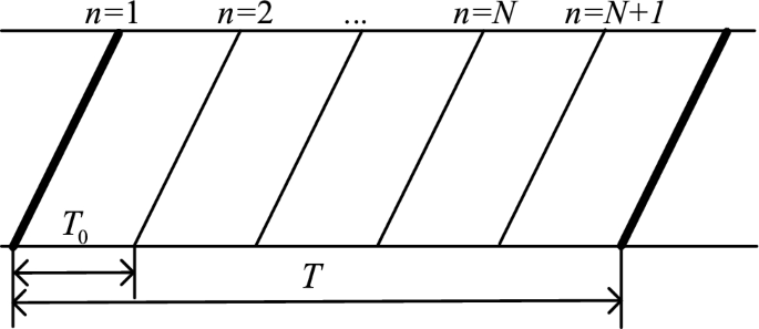

  

  Departure interval of express/local train operation

Generally, the generalized travel cost model for the travel path r between the origin o and destination d consists of riding time, crowding level, waiting time and transfer time.

However, this base model cannot reflect the sensitivity of passenger attributes to each factor, which will be improved next by the questionnaire survey and hybrid model:

$$C_{{\text{r}}}^{{{\text{od}}}} \; = \;\left( {1 + Y_{{\text{r}}}^{{{\text{od}}}} } \right)T_{{\text{r}}}^{{{\text{od}}}} \; + \;W_{{\text{r}}}^{{{\text{od}}}} \; + \;H_{{\text{r}}}^{{{\text{od}}}} \;\forall {\text{r}} \in R_{{{\text{od}}}}$$

(9)

4.3 Structural Equation Modeling

In previous studies, the weight of each factor in the generalized travel cost function is generally chosen as a fixed value. In practice, however, differences in passenger individual attributes and trip attributes may lead to different sensitivities to factors, thus affecting the weight of that factor in the generalized cost function. This paper conducts SEM to explore the perceived heterogeneity of the factors affecting route choice by different travelers in different scenarios with the express/local mode.

SEM could explain the causal relationships among a set of latent variables and between explicit variables and latent variables. A complete SEM includes a measurement model and a structural model. The measurement model quantifies abstract potential variables by establishing the relationship between potential variables and observed variables. Observed variables are selected with reference to previous studies, such as convenience sensitivity corresponding to transfer times [26] and comfort sensitivity corresponding to crowding level [45]. The structural model is mainly used to explore the relationship between explicit and latent variables. In this problem, it is used to explore the relationship between directly observable individual attributes, trip attributes, and perceived latent variables time sensitivity, convenience sensitivity, and comfort sensitivity. Individual attributes and trip attributes are obtained through RP questionnaires for variables such as gender, age, income, career, travel time, travel purpose, and travel distance, while time sensitivity, convenience sensitivity, and comfort sensitivity are estimated by scoring the corresponding aspects on a five-point Likert scale. The SEM framework is as follows (Fig. 5).

Fig. 5

SEM framework

4.4 Hybrid Model

Unlike the commonly used MNL model, the ML model is able to fully characterize the heterogeneity in the traveler choice process by setting the parameters to be estimated as random parameters. Based on the quantification of latent variables by SEM, the hybrid model is able to incorporate the three components of individual and trip attributes, passengers’ sensitivity considering heterogeneity, and route attributes into the analysis. The hybrid model is shown in Fig. 6.

Fig. 6

Hybrid framework

Based on Eq. 10 and the hybrid framework, the travel cost model is formulated as follows:

$$\begin{gathered} V_{{\text{r}}}^{{{\text{od}}}} \; = \;\left( {w_{1} \; + \;Fr_{1} \cdot \eta_{1} } \right) \cdot \left( {T_{{\text{r}}}^{{{\text{od}}}} \; + \;W_{{\text{r}}}^{{{\text{od}}}} } \right)\; + \;\left( {w_{2} \; + \;Fr_{2} \cdot \eta_{2} } \right)H_{{\text{r}}}^{{{\text{od}}}} \hfill \\ \, + \;\left( {w_{3} \; + \;Fr_{3} \cdot \eta_{3} } \right) \cdot Y_{{\text{r}}}^{{{\text{od}}}} T_{{\text{r}}}^{{{\text{od}}}} \; + \;\sum\limits_{{{\text{m}} = 1}}^{{\text{M}}} {B_{{\text{m}}} } \cdot X_{{\text{m}}} \hfill \\ \end{gathered}$$

(10)

where $w_{1}$, $w_{2}$, and $w_{3}$ are the to-be-calibrated coefficients for riding and waiting time, transfer time, and crowding, respectively; $Fr_{1}$, $Fr_{2}$, and $Fr_{3}$ are the to-be-calibrated coefficients for time sensitivity $\eta_{1}$, convenience sensitivity $\eta_{2}$, and comfort sensitivity $\eta_{3}$; X_m is the individual or trip attribute; X₁, X₂, X₃, and X₄ represent gender, age, income, and travel purpose, respectively; B_m is the coefficient for individual or trip attribute; and B₁, B₂, B₃, and B₄ represent the coefficients for gender, age, income, and travel purpose, respectively.

4.5 Passenger Flow Distribution Calculation

The probability of route choice is calculated based on the generalized travel cost. The MNL model, which is often applied to passenger flow assignment, requires “absolute differences in utility” because of the IIA property [46], whereas in this problem, the express and local travel routes on municipal rail transit are closely related to each other. Teng et al. [1] found that using relative values of utility in the model can better present the dynamics of route choice:

$$P_{{\text{r}}}^{{{\text{od}}}} \; = \;\frac{{\exp \;\left( {\lambda V_{{\text{r}}}^{{{\text{od}}}} /\overline{V}^{{{\text{od}}}} } \right)}}{{\sum\limits_{{{\text{r}} \in R_{{{\text{od}}}} }} {\exp \;\left( {\lambda V_{{\text{r}}}^{{{\text{od}}}} /\overline{V}^{{{\text{od}}}} } \right)} }}$$

(11)

where $\overline{V}^{{{\text{od}}}}$ is the average value of the combined utility of all valid paths between starting point o and ending point d.

The static flow assignment problem can be considered a fixed-point problem in nature [46], represented using $x = F(x)$. There exists a scheme equilibrium value x (meaning passenger flow) on the path, and when the passenger flow solved at one step is entered into the algorithm, the passenger flow in the next step does not change, or the change is less than some threshold value. This means that the solution to this problem (i.e., the fixed point of existence) is found, i.e., the passenger flow x is entered into the iterative operator or the mapping function where the passenger flow is no longer changing.

The method of successive averages (MSA) algorithm flow is as follows (Fig. 7):

Fig. 7

MSA algorithm flow

Solving steps:

• (1) Determine the effective path between od pairs.

• (2) In general, the total od demand corresponding to multiple paths in static passenger flow assignment is fixed, according to which the initial value of passenger flow of each path is set.

• (3) Calculate the utility of the route based on the initial route passenger flow $C\left( {x^{{\text{n}}} } \right)$, marked as y.

• (4) Use the MSA algorithm to determine the search direction of the next cycle x:

  $$x^{{{\text{n}} + 1}} \; = \;x^{n} \; + \;\frac{1}{n}\;\left( {y^{{\text{n}}} \; - \;x^{{\text{n}}} } \right)$$

  (12)

• (5) Substitute $C\left( {x^{{\text{n}}} } \right)$ into the logit model to calculate the new route choice probability, and multiply it by the od amount to obtain the new assigned passenger flow.

• (6) To check whether the new assigned passenger flow is converged, the following methods can be used.

If g(n) < e, complete and output the current passenger flow; otherwise, set n = n + 1 to repeat the fourth and fifth steps.

5 Study Area and Survey Design

5.1 Study Area

Municipal rail transit provides a fast and convenient connection between urban centers and surrounding clusters. In this paper, a municipal rail line serving distant suburban groups in Shanghai is selected as the study area, operating both express trains and local trains. The line starts from Longyang Road Station in the north and ends at Dishui Lake Station in the south, with a total length of 58.96 km and 13 stations with a station distance of 3 km or more. The station spacing is within the scope of the municipal rail transit line regulations, and the line has obvious characteristics of the municipal rail transit line.

Figure 8 shows the distribution of local train stations and express train stations in the study area, with arrows indicating the od stations where passengers depart and arrive.

Fig. 8

Study area

Figure 9 shows the ridership of the municipal rail transit line on a weekday. On weekdays, the ridership of the study area exhibits a two-way peak curve with obvious morning and evening peaks, reflecting this line plays a critical role in passengers’ daily commute.

Fig. 9

Ridership of case line on a weekday

Figure 10 displays the production and attraction ridership at each station along the line. The volume of the station ridership is represented by color and thermal radius, where the latter indicates the relative value of ridership between stations without absolute significance. It can be seen that the difference between the inbound and outbound passenger flow of each station is not significant, which means that the production and attraction of passenger flow of each station are balanced. The inbound and outbound passenger flow of Huinan, Zhou Pudong, Hesha Hangcheng, and Xinchang in the middle part of the line are larger, which indicates that the municipal rail transit line has to ensure the high frequency of short-distance and large-passenger traffic, but also to take into account the short time travel of long-distance and small-passenger traffic.

Fig. 10

Station production ridership and attraction ridership heatmap

5.2 Survey Design

The questionnaire consisted of four main parts: an RP survey on the most frequent trips, an SP survey on the choice of express and local trains, sensitivity perception survey, and participants’ demographic and socioeconomic characteristics.

The first part of the questionnaire is the basic information about the most frequent trip, including travel time, period, purpose, distance, and number of transfers. The second part consists of a set of express and local train choice experiments. The SP questionnaire design includes four aspects: option design, attribute design, level design, and scenario design. In terms of the option design, for passenger types of different origin and destination stations, the express and local train riding options are set as express train only, local train only, express train to local train, and local train to express train. Because of the assumption in previous studies that passengers should not transfer more than once between express and local train routes [8], and the practical context of the case in this paper, passengers are considered to have at most one transfer in the option design. For the level design of each attribute, the questionnaire combines the actual level and floating range of each attribute, with time information referring to Shentong Metro and Gaode Map. For the scenario design, an orthogonal experimental design is used to ensure sample representativeness. Table 4 shows the attributes and levels of the SP questionnaire.

Table 4 The attributes and levels of the SP questionnaire

The third part is about individual sensitivity perception, with measurement dimensions and content in Table 5. A five-point Likert scale is developed to assess passengers’ conformity levels in relation to time, transfer, and comfort sensitivity based on their daily travel experiences. The scale ranges from 1 (very nonconforming) to 5 (very conforming), with higher scores indicating greater conformity.

Table 5 Measurement dimensions and content

At the end of the questionnaire, respondents are asked to describe their sociodemographic profile (including gender, age, income, and career).

6 Results

6.1 Descriptive Analysis

We conducted the survey along Shanghai Metro Line 16, which has significant express and local train mode characteristics, and collected a total of 550 questionnaires. The survey plan and design were supervised by Shanghai Shentong Metro, and the questionnaire was released in August and September 2022 with the support of a professional survey company. For questionnaire quality, specific questions were set up to detect respondents’ concentration and consistency. By checking the answering time and the answering logics, invalid answers were eliminated, and 502 (91.27%) were valid answers for analysis. Based on the principle of orthogonal design, 48 scenarios were generated for the SP survey using JMP statistical analysis software. To ensure respondents’ focus, we divided the 48 scenarios into three groups, each containing 16 orthogonal scenarios.

Calculating an appropriate sample size is a crucial step in conducting formal surveys. An excessively large sample size can increase survey costs and subsequent data processing workload, while a sample size that is too small can result in reduced representativeness and an inability to fully reflect data characteristics. From a statistical perspective, the rationality of sample size selection is mainly based on two indicators: confidence level and allowable error. The sample size estimated by the random sample method is typically used in surveys conducted through random sampling. The calculation formula is as follows:

$$n \ge \frac{{Z^{2} p\left( {1 - p} \right)}}{{E^{2} }}$$

(13)

In the formula, Z represents the statistical value corresponding to the confidence level; p represents the standard deviation, which is generally 0.5; and E represents the relative allowable error range for sampling. When the confidence level is 95%, Z is 1.96, the p value is 0.5, and the E value is 5%; the sample size should be no less than 385. The sample size in this article meets the standard. Participants’ demographic and socioeconomic characteristics are shown in Table 6.

Table 6 Participants’ demographic and socioeconomic characteristics

To test the representativeness of the sample of this survey, we combined Shanghai population census data, Shanghai Line 16 passenger flow data, and the results of a related survey [25], which was approved by Tongji University, to test the sampling structure. This related survey limits the respondents to those who are familiar with the Shanghai Metro, which is an important reference for this questionnaire.

• (1) Gender structure: According to the Seventh National Population Census of Shanghai, 51.8% of the city’s resident population is male, and 48.2% is female. According to the reference investigation in Shanghai, the percentage of male and female metro passengers is 47.30% and 52.70%, respectively [25]. The gender structure of our questionnaire is similar to the above.

• (2) Age structure: According to the reference investigation in Shanghai, metro passengers under the age of 18, 18–40, 41–60, and over the age of 60 account for 2.53%, 83.71%, 12.87%, and 0.89%, respectively [25]. The age structure of our questionnaire is similar to the above.

• (3) Travel time period: The peak hour factor for line passenger volume is the ratio of peak hour line passenger volume to the total full-day line passenger volume, reflecting overall travel time period characteristics. The peak hour factor in the related survey is 46.32%, differing very little from 48.17% in ours.

From the perspective of gender, the proportion of male and female respondents is relatively balanced. In terms of age, the age distribution is 18–30 and 31–40 years old, and most of them are young and middle-aged passengers. The majority of people have income of 5001–10,000, 10,001–20,000, or more than 20,000 per month, and the number of people is evenly distributed across the three categories. The reason for using rail transit among respondents is mainly for commuting, and the travel period is greater in the morning peak.

6.2 Reliability test analysis

• (1)
  

  Reliability and validity

  As for the reliability test, the most common method of reliability testing is based on internal consistency coefficients, mainly based on Cronbach’s coefficient $\alpha$. Generally speaking, the overall coefficient should preferably be above 0.8, and between 0.7 and 0.8 is acceptable, while the reliability coefficient of subscales should preferably be above 0.7, and between 0.6 and 0.7 is acceptable.

  $$\alpha \; = \;\frac{K}{K - 1}\;\left( {1\; - \;\frac{{\sum {{\text{S}}_{{\text{i}}}^{2} } }}{{{\text{S}}^{2} }}} \right)$$

  (14)

  where K² is the number of questions on the scale, S_i² is the variance of the ith question, and S² is the total variance within the scale. The Cronbach coefficients for the three dimensions including time sensitivity, convenience sensitivity, and comfort sensitivity are 0.62, 0.71, and 0.78, respectively, passing the reliability test.

  The validity test is generally based on the Kaiser–Meyer–Olkin (KMO) measure and Bartlett’s spherical test. A KMO value greater than 0.6 and a p-value less than or equal to 0.05 for Bartlett’s spherical test indicate that the scale is suitable for factor analysis and can effectively measure the target (Table 7).

  Table 7 KMO and Bartlett’s test

• (2)
  

  Factor analysis

  Because of the lack of a common standard for route choice sensitivity index with the express and local trains, exploratory factor analysis is applied to verify the appropriateness of each latent variable with its measurement index. By using principal component analysis to select the factors, the factors with eigenvalues greater than 1 are extracted, which are time sensitivity, convenience sensitivity, and comfort sensitivity. For all factor loadings above 0.7, indicating valid measurement topics for each latent variable, rotated load matrices are shown in Table 8.

  Table 8 Rotated component matrix

• (3) SEM parameter calibration

  Specifically, there is a strong correlation between period and purpose, such as the peak hour travel purpose being mainly commuting, and only the travel purpose is retained in SEM. In addition, three sets of covariates are added between age, income, and travel purpose, as shown in Fig. 5. The evaluation indicators indicate that SEM passes the test (Table 9).

  Table 9 Evaluation indicator value

We quantify the latent variables based on the relationship between the latent variables and the observed variables in the results of SEM. After normalizing the path factor loadings between the latent and observed variables, the quantitative results for each latent variable (time sensitivity $\eta 1$, convenience sensitivity $\eta 2$, and comfort sensitivity $\eta 3$) are as follows.

$$\begin{gathered} \eta 1\; = \;0.26 \cdot A1\; + \;0.25 \cdot A2\; + \;0.49 \cdot A3 \hfill \\ \eta 2\; = \;0.30 \cdot A4\; + \;0.37 \cdot A5\; + \;0.33 \cdot A6 \hfill \\ \eta 3\; = \;0.36 \cdot A7\; + \;0.32 \cdot A8\; + \;0.32 \cdot A9 \hfill \\ \end{gathered}$$

(15)

The standardized parameter results are shown in Table 10.

Table 10 Standardized parameter results

The relationship between individual attributes and sensibilities can be reflected by the standard path coefficient values. For example, the standardized path coefficient value of age for time sensitivity is less than zero, while convenience sensitivity and comfort sensitivity are over zero, thus indicating that older people tend to have higher requirements for convenience and comfort level, but not time sensitivity. For every age level increase, time sensitivity decreases by 0.078, convenience sensitivity increases by 0.169, and comfort sensitivity increases by 0.126. Table 10 reflects and quantifies the relationship between the effect of individual attributes, trip attributes, and factor sensitivities, which is crucial for constructing a route travel cost function taking heterogeneity into account. Furthermore, we establish the interplay between these factors and sensitivity, which can provide insights into the preferences of distinct passenger groups in selecting express and local trains across various travel contexts.

6.3 Hybrid Model Estimates

Based on the survey data, combined with the results of the SEM, the passengers’ sensitivity is added to the coefficients of riding time, transfer time, and comfort of the utility equation to study the heterogeneity of passengers. The results of the discrete choice model parameter calibration are shown in Table 11.

Table 11 Hybrid model parameter calibration results

In Table 11, NsB₂ and NsB₄ are the standard deviations of age and trip purpose. Since the mean and standard deviation of age and trip purpose are significant, B₂ and B₄ are the random parameters in the model.

To verify the explanatory power of the model, the MNL model and ML model are used as base models. For the same choice problem, the different models are comparable to each other [47]. The log-likelihood function value and Akaike information criterion (AIC) are shown in Table 12. The hybrid model has smaller absolute value of log-likelihood and smaller value of AIC, indicating that the model fits significantly better. Moreover, the mean and standard deviation of the random parameters (B₂ and B₄) are significant, indicating that the model can portray passenger heterogeneity and has greater explanatory power.

Table 12 Comparison between the base model and our hybrid model

6.4 Variable Effect Analysis

According to the type of origin and destination stations, three groups of cases are set up, corresponding to the scenarios of the express station to express station, express station to local station, and local station to express station. There are more route options from express station to express station, as a case study for the following analysis.

The route choice probability and flow assignment results for passengers are calculated based on the hybrid model and MSA algorithm. Meanwhile, the results of the route choice probability for the baseline group are displayed in Table 13, where the average of each continuous variable and the value with the largest percentage of each categorical variable form its attributes.

Table 13 Example calculation results

Based on the relationship between the impact of different individual attributes and trip attributes on sensitivity in Table 10, and the hybrid model calibration results, we compare the differences in the route choice probabilities of different characteristic groups, as shown in Table 14. A single-factor sensitivity analysis is conducted for age and income for several levels separately, as shown in Fig. 11.

Table 14 Calculation results for different passenger groups

Fig. 11

Sensitivity analysis of age and income

• (1) Gender

  Gender affects the probability of route choice to a small degree, with males having a higher probability of route choice for local train transfers to express trains than females.

• (2) Age

  With increasing age, passengers’ sensitivity to comfort and convenience increases, while time sensitivity decreases. The young have a significantly higher preference for express trains and local train transfers to express trains than the elderly, with a difference of 10.22% in the probability of choosing express trains. The magnitude of the increase or decrease in probability grows progressively with increasing age. Eventually, the route choice probability in the elderly group shows a pattern of "medium probability express–medium probability local–low probability local transfer to express" with two principal and one auxiliary.

• (3) Income

  With increasing income, passengers’ probability of choosing express trains increases, the probability of choosing local trains decreases, and the impact on the probability of choosing transfers is small. As can be seen in Fig. 11, the growth rate of the probability of choosing express trains and the decrease rate of the probability of choosing local trains continue accelerating among high-income passengers. Eventually, the probabilities in the high-income group show a "high probability express–medium probability local transfer to express–low probability local" stepped pattern.

• (4) Purpose

  As can be seen from the path normalization parameters between travel purpose and sensitivity in Table 10, travel purpose has a significant impact on sensitivity. Commuter passengers prioritize time and convenience, while non-commuter passengers value comfort as their primary concern. Compared with commuter passengers in the baseline group, non-commuter passengers have a significantly higher probability of local trains, with a gap of 10.96% and a growth rate of 54.37%, and a significantly lower probability of express trains, with a gap of 11.36% and a decline rate of 22.91%. Travel purpose shows strong passenger heterogeneity in the express and local route choice process.

• (5) Travel distance

  The analysis regarding the above four attributes is based on the hybrid model with fixed origin and destination stations for route choice. In the following, considering the effect of travel distance on preferences for express trains, the maximum time passengers wait for express trains is explored for different travel distances.

  Case B: Express station to express station (Xinchang–Longyang Road)

  Case C: Express station to express station (Luoshan Road–Longyang Road)

  In case B, when the distance is shortened to about 50% of the whole trip from Xinchang to Longyang Road, regression analysis is performed based on the maximum express train waiting time chosen by passengers and the corresponding choice probability. The cumulative frequency distribution obtained is shown in Fig. 12a. This curve can be interpreted with the help of the concept of price sensitivity. The point where the curve grows at the maximum rate can be set as p. The maximum waiting time for the express train has the most passengers in the small interval centered on p. As the waiting time increases, it gradually reaches the upper limit of passengers’ patience, thus abandoning the path of waiting for the express train due to the long waiting time.

  Fig. 12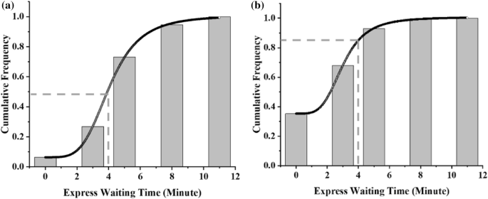

  

  Express waiting time cumulative frequency distribution: a Case B: Xinchang–Longyang Road, b Case C: Luoshan Road–Longyang Road

  Similarly, Fig. 12b shows the cumulative frequency distribution of the express train waiting time for the case C scenario, with the distance reduced to about 20% of the whole trip.

  In case B, more than 50% of passengers are willing to wait more than 4 min for the express train, while in case C, less than 20% of passengers are willing to wait more than 4 min for the express train.

  According to the characteristics of the cumulative distribution curve of probability density, we try to test whether it is a normal distribution. In the case of a small sample size, the Shapiro–Wilk (S-W) test is usually used, and the obtained significance parameters are as follows (Table 15).

  Table 15 S-W test significance parameters

  The significance test p-value is greater than 0.05, indicating that the data satisfy a normal distribution. From this, it can be obtained that the upper limit of passengers’ waiting time for express trains obeys a normal distribution. The mean value of the normal distribution decreases as the traveling distance shortens. We can interpret this upper limit of waiting time as the passengers’ tolerance for waiting on express trains. The waiting tolerance of passengers increases as their travel distance lengthens. In other words, passengers who travel longer distances have a stronger desire to wait for the express train.

• (6) Multi-attribute combination analysis

  The distribution of group characteristics is strongly related to the type of station, with Station A located in a high-tech industrial area with a predominantly young commuter group, and Station B located in an old urban residential area with a predominantly older non-commuter group. Table 16 shows the route choice distribution characteristics of the groups around the stations in this context. Analyzing the express and local train choice behavior based on the station type and the passenger type in the surrounding area is an important reference when setting up express train stops and the ratio of express and local train departures in different time periods.

  Table 16 Age and income sensitivity analysis

By combining the od volume of Shanghai Metro passenger flow with the probability of express and local train route choice, a passenger flow assignment algorithm is used to calculate the interval passenger flow for a given peak hour and off-peak hour. Table 17 presents the passenger flow results for several key intervals, finding that the hybrid model results are closer to the actual observations than the traditional MNL model.

Table 17 Passenger flow distribution result verification

Figure 13 shows the heat map of passenger flow corresponding to the peak and off-peak hours, and it is found that "East Zhoupu–Luoshan Road" and "Heshahangcheng–East Zhoupu" are popular sections. Especially for these popular sections during the peak period, it is crucial to prioritize sufficient transportation capacity and elevate service quality through operational plan adjustments or service facility upgrades.

Fig. 13

Heat map for interval passenger flow calculation (peak and off-peak hours)

7 Discussion

• (1) Express station setting

  Our analysis reveals that elderly passengers seek a convenient and comfortable travel experience. The elderly are almost twice as likely as the young to choose direct local trains. Routes including express trains (direct express trains, transfer express trains) are significantly less attractive to the elderly than to the young. Express station settings could be targeted towards stations where young commuters predominate.

  Moreover, high-income passengers are more likely to pursue a fast and comfortable travel experience. Passengers in the high-income category are more likely to choose routes including express trains (direct express trains, transfer express trains). To better satisfy this type of travel need, municipal rail transit should focus on improving service quality. For example, providing value-added services by operating full-distance trains (with no stop) can help balance operating costs and ensure that the pricing strategies match the preferences of different passenger groups.

  The heterogeneity of passengers is also impacted by the differences in travel distance. The maximum waiting time for express trains is around 8–10 min for most passengers. As the travel distance increases, the upper limit of passengers’ waiting time also gradually increases, indicating that long-distance passengers are more willing to ride express trains. In the formulation of the stop plan for express trains, it is recommended that greater consideration be given to stations located near the two ends of the line. Such an approach can enhance the efficiency and attractiveness of express train services for long-distance commuters while still catering to the diverse travel needs of passengers.

• (2) Express and local train operation scheme

  During peak periods, with commuters’ travel demand for rapidity as the main focus, the frequency of express train departures can be increased while ensuring transportation capacity. During off-peak periods, due to decreased ridership, the departure scale of express and local trains can be appropriately reduced. Mostly shopping and leisure passengers or residents in the local living circle have minor differences in the probability of choosing each route type. The proportion of express trains can be reduced to save operating costs. Moreover, it is recommended that small-crossing trains covering commercial centers and that nearby residential areas be operated during off-peak period to meet non-commuters’ travel demand while reducing wasted capacity on the entire length of the operation. Such changes may help to optimize the efficiency and effectiveness of transit services while still meeting the diverse travel needs of passengers.

• (3) Transfer passenger service

  Compared to other passenger age groups, young passengers are less sensitive to transfers; however, they have increased sensitivity to transfers when commuting. This is most likely due to concerns about the uncertainty of the arrival of following trains, which creates potential travel cost. To heighten the transfer experience for passengers during peak hours, it is essential to provide accurate and timely transfer information for passengers to make proper route choice decisions. Making full use of information induction for municipal rail transit with express/local modes is very important.

8 Conclusion

This study investigated the effect of passengers’ heterogeneity on route choice behavior with express and local trains. Based on the RP and SP survey data, we proposed the hybrid model combining SEM and the ML model. It correlated the sensitivity of individual attributes, trip attributes, and key factors of route choice (time, comfort, and convenience) to support route choice probabilities for express and local trains considering heterogeneity. By exploring passenger choice behavior in terms of individual perception, this approach focused on various types of passenger preferences. The proposed model was applied to the municipal rail transit in Shanghai, providing practical and scientifically grounded insights for transit planners and policymakers. Main conclusions can be drawn according to the different types of passenger heterogeneity as follows:

• (1) The individual attributes income and age, as well as trip attributes purpose and distance, have a significant effect on the sensitivity of factors in route choice. Passenger heterogeneity does play a crucial role in their corresponding preferences for express and local trains.

• (2) Trip purpose has the greatest impact on sensitivity among all attributes. The same group has a significantly higher preference for express trains when commuting, with an 11.36% gap in the probability of choosing express trains in this case.

• (3) Compared to other individual attributes, age impacts sensitivity to a greater extent. The young have a significantly higher preference for express trains than the elderly, with a difference of 10.22% in the probability of choosing express trains. Moreover, the young are less sensitive to transfers than the elderly; however, they have increased sensitivity to transfers when commuting.

• (4) For most passengers, the maximum wait time for express trains is about 8–10 min. As the travel distance increases, the maximum time passengers wait for the express train gradually increases.

The hybrid model provides modeling and prediction for exploring the express and local train choice behavior of groups with different attributes. This paper provides suggestions for express station settings, large and small crossings, the ratio of express and local trains, and the operating frequency, which are the key elements of the municipal rail transit operation scheme. It helps to support passenger services and adjust operation schemes to focus on different passenger groups over time. This paper also provides a research basis and research ideas for rail transportation service supply and demand balance studies.

There are still several issues that need to be addressed in further work. Route choice behavior and train operation scheme interact with each other. Our research mainly focuses on refining passenger preferences to study route choice behavior, providing demand-side support for train operating schemes. How to take into account the relationship between supply and demand in formulating operation organization will be the focus of our further study.

References

Teng J, Hui W, Zhang C, Liu S (2021) Evaluation of operating schemes on municipal rail transit with express/local mode. Transp Res Rec J Transp Res Board 2675:583–597. https://doi.org/10.1177/03611981211030261
Cats O, Wang Q, Zhao Y (2015) Identification and classification of public transport activity centres in Stockholm using passenger flows data. J Transp Geogr 48:10–22. https://doi.org/10.1016/j.jtrangeo.2015.08.005
Baek J, Sohn K (2016) An investigation into passenger preference for express trains during peak hours. Transportation 43:623–641. https://doi.org/10.1007/s11116-015-9592-3
Tang L, D’Ariano A, Xu X et al (2021) Scheduling local and express trains in suburban rail transit lines: mixed–integer nonlinear programming and adaptive genetic algorithm. Comput Oper Res 135:105436. https://doi.org/10.1016/j.cor.2021.105436
Chen J, Pu Z, Guo X et al (2023) Multiperiod metro timetable optimization based on the complex network and dynamic travel demand. Phys A 611:128419. https://doi.org/10.1016/j.physa.2022.128419
Tang L, Xu X (2022) Optimization for operation scheme of express and local trains in suburban rail transit lines based on station classification and bi-level programming. J Rail Transp Plan Manag 21:100283. https://doi.org/10.1016/j.jrtpm.2021.100283
Di D, Yang D (2014) Passenger flow analysis model about express/slow train in urban rail transportation corridor. J Tongji Univ Natl Sci 42:78–83
Xie X, Zhang X, Chen J et al (2014) The discrete choice model of urban rail transit passengers’ route choice. J Transp Syst Eng Inf Technol 14:127–131
Zhao X, Sun Q, Ding Y et al (2016) Passenger choice behavior for regional rail transit under express/local operation with overtaking. J Transp Syst Eng Inf Technol 16:104–109
Bekhor S, Prato CG (2009) Methodological transferability in route choice modeling. Transp Res Part B Methodol 43:422–437. https://doi.org/10.1016/j.trb.2008.08.003
Amirgholy M, Gonzales EJ (2017) Efficient frontier of route choice for modeling the equilibrium under travel time variability with heterogeneous traveler preferences. Econ Transp 11–12:1–14. https://doi.org/10.1016/j.ecotra.2017.09.001
Leng J, Zhai J, Li Q, Zhao L (2018) Construction of road network vulnerability evaluation index based on general travel cost. Phys A 493:421–429. https://doi.org/10.1016/j.physa.2017.11.018
Feng Y, Zhao J, Sun H et al (2022) Choices of intercity multimodal passenger travel modes. Phys A 600:127500. https://doi.org/10.1016/j.physa.2022.127500
Teng J, Liu W-R (2015) Development of a behavior-based passenger flow assignment model for urban rail transit in section interruption circumstance. Urban Rail Transit 1:35–46. https://doi.org/10.1007/s40864-015-0002-0
Larsen OI, Sunde Ø (2008) Waiting time and the role and value of information in scheduled transport. Res Transp Econ 23:41–52. https://doi.org/10.1016/j.retrec.2008.10.005
Fernández E, Joaquín C (1993) Transit assignment for congested public transport systems: an equilibrium model. Transp Sci 2:133–147
Gao Y, Yang L, Gao Z (2018) Energy consumption and travel time analysis for metro lines with express/local mode. Transp Res Part D Transp Environ 60:7–27. https://doi.org/10.1016/j.trd.2016.10.009
Li Z, Mao B, Bai Y, Chen Y (2019) Integrated optimization of train stop planning and scheduling on metro lines with express/local mode. IEEE Access 7:88534–88546. https://doi.org/10.1109/ACCESS.2019.2921758
Zhang H, Han B (2019) Optimizing Train plan of express-local modes for suburban rail transit. In: 2019 4th international conference on electromechanical control technology and transportation (ICECTT). pp 336–340
Si B, Mao B, Liu Z (2007) Passenger flow assignment model and algorithm for urban railway traffic network under the condition of seamless transfer. J China Railw Soc 29:12–18
Pel AJ, Bel NH, Pieters M (2014) Including passengers’ response to crowding in the Dutch national train passenger assignment model. Transp Res Part A Policy Pract 66:111–126. https://doi.org/10.1016/j.tra.2014.05.007
Douglas N, Karpouzis G (2006) Estimating the passenger cost of train overcrowding
Lam S-H, Xie F (2002) Transit path-choice models that use revealed preference and stated preference data. Transp Res Rec 1799:58–65. https://doi.org/10.3141/1799-08
Guo Z, Wilson NHM (2011) Assessing the cost of transfer inconvenience in public transport systems: A case study of the London underground. Transp Res Part A Policy Pract 45:91–104. https://doi.org/10.1016/j.tra.2010.11.002
Cheng Y, Ye X, Fujiyama T (2022) How does interchange affect passengers’ route choices in urban rail transit? A case study of the Shanghai Metro. Transp Lett 14:416–426. https://doi.org/10.1080/19427867.2021.1883803
Walker JL (2001) Extended discrete choice models: integrated framework, flexible error structures, and latent variables. Massachusetts Institute of Technology, Cambridge
Prato CG, Bekhor S, Pronello C (2005) Methodology for exploratory analysis of latent factors influencing drivers’ behavior. Transp Res Rec 1926:115–125. https://doi.org/10.1177/0361198105192600114
Prato CG, Bekhor S, Pronello C (2012) Latent variables and route choice behavior. Transportation 39:299–319. https://doi.org/10.1007/s11116-011-9344-y
Lu K, Han B, Zhou X (2018) Smart urban transit systems: from integrated framework to interdisciplinary perspective. Urban Rail Transit 4:49–67. https://doi.org/10.1007/s40864-018-0080-x
Kurauchi F, Schmöcker J-D, Fonzone A et al (2012) Estimating weights of times and transfers for hyperpath travelers. Transp Res Rec J Transp Res Board 2284:89–99. https://doi.org/10.3141/2284-11
Liu W, Liu X (2016) Route choice research in rail transit network based on passenger classification. J Transp Eng Inf 14:81–86
Abou-Zeid M, Ben-Akiva M, Bierlaire M et al (2010) Attitudes and value of time heterogeneity. Applied transport economics–a management and policy perspective. De Boeck Publishing, Stockholm Sweden
Zhao P, Qu R, Song W (2019) Passenger choice behavior of high-speed railway considering individual heterogeneity. J Beijing Jiaotong Univ 43:117
Liu J, Hao X (2019) Travel mode choice in city based on random parameters logit model. J Transp Syst Eng Inf Technol 19:108
Cascetta E, Russo F, Viola FA, Vitetta A (2002) A model of route perception in urban road networks. Transp Res Part B Methodol 36:577–592. https://doi.org/10.1016/S0191-2615(00)00041-2
Domencich TA, McFadden D (1977) Urban travel demand–a behavioral analysis. Can J Econ 10:724
Koppelman FS, Sethi V (2005) Incorporating variance and covariance heterogeneity in the generalized nested logit model: an application to modeling long distance travel choice behavior. Transp Res Part B Methodol 39:825–853. https://doi.org/10.1016/j.trb.2004.10.003
Mwale M, Luke R, Pisa N (2022) Factors that affect travel behaviour in developing cities: a methodological review. Transp Res Interdiscip Perspect 16:100683. https://doi.org/10.1016/j.trip.2022.100683
Bekhor S, Reznikova L (2007) Application of cross-nested logit route choice model in stochastic user equilibrium traffic assignment. Transp Res Rec J Transp Res Board 2003:41–49
Zhou Z, Chen A, Bekhor S (2012) C-logit stochastic user equilibrium model: formulations and solution algorithm. Transportmetrica 8:17–41. https://doi.org/10.1080/18128600903489629
Ben-Akiva M, Bierlaire M (1999) Discrete choice methods and their applications to short term travel decisions. In: Hall RW (ed) Handbook of transportation science. Springer, Boston, MA, pp 5–33
Krueger R, Bierlaire M, Daziano RA et al (2021) Evaluating the predictive abilities of mixed logit models with unobserved inter- and intra-individual heterogeneity. J Choice Model 41(1–2):100323. https://doi.org/10.1016/j.jocm.2021.100323
Tang L, Xu X (2018) Study of suburban passengers’ route choice behavior under express/local train mode. J Wuhan Univ Technol 42:947–951
Shang W, Han K, Ochieng W, Angeloudis P (2017) Agent-based day-to-day traffic network model with information percolation. Transportmetr A Transp Sci 13:38–66. https://doi.org/10.1080/23249935.2016.1209254
Pan H, Li J, Chen P (2016) Study on the ownership of motorized and non-motorized vehicles in suburban metro station areas: a structural equation approach. Urban Rail Transit 2:47–58. https://doi.org/10.1007/s40864-016-0037-x
Paetz F, Steiner WJ (2018) Utility independence versus IIA property in independent probit models. J Choice Model 26:41–47. https://doi.org/10.1016/j.jocm.2017.06.001
Teng J, Xue H (2020) A study on intercity travel choice behavior based on traveler heterogeneity. Railw Transp Econ 42:60–66
Funding
The authors disclose receipt of the following financial support for the research, authorship, and/or publication of this article: This research was supported by Research on suburban railway operation management system under the background of integration of Yangtze River Delta (2021F023).
Author information
Authors and Affiliations
Corresponding author
Ethics declarations
Conflict of interest
The authors declare no potential conflicts of interest with respect to the research, authorship, and/or publication of this article.
Additional information
Communicated by Baoming Han.
Rights and permissions
Open Access This article is licensed under a Creative Commons Attribution 4.0 International License, which permits use, sharing, adaptation, distribution and reproduction in any medium or format, as long as you give appropriate credit to the original author(s) and the source, provide a link to the Creative Commons licence, and indicate if changes were made. The images or other third party material in this article are included in the article's Creative Commons licence, unless indicated otherwise in a credit line to the material. If material is not included in the article's Creative Commons licence and your intended use is not permitted by statutory regulation or exceeds the permitted use, you will need to obtain permission directly from the copyright holder. To view a copy of this licence, visit http://creativecommons.org/licenses/by/4.0/.
About this article
Cite this article
Peng, W., Teng, J. & Wang, H. Understanding Heterogeneous Passenger Route Choice in Municipal Rail Transit with Express and Local Trains: An Empirical Study in Shanghai. Urban Rail Transit (2024). https://doi.org/10.1007/s40864-024-00214-8
Received:
Revised:
Accepted:
Published:
DOI: https://doi.org/10.1007/s40864-024-00214-8