Adopting Quaternion Wavelet Transform to Fuse Multi-Modal Medical Images

Abstract

Medical image fusion plays an important role in clinical applications such as image-guided surgery, image-guided radiotherapy, noninvasive diagnosis, and treatment planning. In this paper, we propose a novel multi-modal medical image fusion method based on simplified pulse-coupled neural network and quaternion wavelet transform. The proposed fusion algorithm is capable of combining not only pairs of computed tomography (CT) and magnetic resonance (MR) images, but also pairs of CT and proton-density-weighted MR images, and multi-spectral MR images such as T1 and T2. Experiments on six pairs of multi-modal medical images are conducted to compare the proposed scheme with four existing methods. The performances of various methods are investigated using mutual information metrics and comprehensive fusion performance characterization (total fusion performance, fusion loss, and modified fusion artifacts criteria). The experimental results show that the proposed algorithm not only extracts more important visual information from source images, but also effectively avoids introducing artificial information into fused medical images. It significantly outperforms existing medical image fusion methods in terms of subjective performance and objective evaluation metrics.

1 Introduction

Various medical image modalities are available, including magnetic resonance imaging (MRI), computed tomography (CT), ultrasonography, magnetic resonance angiography (MRA), positron emission tomography (PET), single-photon emission CT (SPECT), and functional MRI (fMRI) [1]. These modalities provide different information about human organs and have their respective application ranges. For example, CT and MRI can show anatomical information of the viscera with high spatial resolution. Despite the low spatial resolution of PET, it can provide function information on the viscera’s metabolism. There are some differences between CT and MRI. CT images can show dense structures such as bones and implants with less distortion, but they cannot be used to detect physiological changes. Whereas MRI can provide normal and pathological soft tissue information, but it cannot show information regarding bones. Hence, in clinical applications, a single modality is insufficient to provide doctors with sufficient information to diagnose a patient’s condition. It is necessary to combine several imaging modalities into one image to obtain more accurate information. The physician can accurately diagnose a disease and choose an appropriate therapeutic schedule according to comprehensive information of diseased tissue or organs in fused images. Therefore, it is necessary to fuse multi-modal medical images [2, 3].

Image fusion can be broadly defined as the process of combing multiple input images or some of their features into a single image without the introduction of distortion or loss of information [4]. Recently, a lot of medical image fusion methods based on multiscale geometry analysis have been proposed. Examples include medical image fusion algorithms based on wavelets [5], ripplet transform [6], contourlet transform [7], nonsubsampled contourlet transform (NSCT) [8], and shearlet transform [9]. The NSCT, as a fully shift-invariant form of the contourlet transform, leads to better frequency selectivity and regularity. The shearlet transform forms a tight frame at various scales and directions, and is optimally sparse for representing images with edges. Although the NSCT and the shearlet transform are fully shift-invariant, they have redundancies and thus fusion methods based on NSCT and Shearlet are slower than other multiscale decomposition (MSD) methods, such as those based on the contourlet and wavelet transforms. The contourlet transform offers flexible multi-resolution and multi-directional decomposition for images. The discrete wavelet transform (DWT) preserves different frequency information in stable form and allows good localization both in the time and spatial frequency domains. However, one of the major drawbacks of DWT and the contourlet transform is lack of shift invariance. Therefore, image fusion method [5–7] performance quickly deteriorates when there is slight object movement or when the source multi-modal images cannot be perfectly registered. The quaternion wavelet transform (QWT) [10], proposed by Corrochano, is a new multiscale analysis tool for capturing the geometry features of an image. The QWT coefficients have three phases and a magnitude [11]. The first two QWT phases encode the shift of image features in the horizontal and vertical coordinate system, respectively. The third phase encodes the edge orientation mixtures and texture information. Hence, the QWT is nearly shift-invariant. The QWT also inherits many other interesting and useful theoretical properties, such as the quaternion phase representation and symmetry properties. The QWT subbands, as the quaternion analytic signals, contain rich geometric information of source medial images. Furthermore, the QWT can be computed using a two-dimensional (2-D) dual-tree filter bank with linear computational complexity.

Except for the MSD tool, the fusion rule is regarded as the most important factor that observably influences fusion performance. Generally, the classic fusion rules include standard deviation, spatial frequency, and average gradient. Fusion rules based on principal component analysis methods lead to pixel distortion in fused multi-modal medical images [6]. In [12], a visibility feature method was proposed to fuse the quaternion wavelet coefficient of source medical images. However, the fused images had lower contrast because the visibility feature does not effectively select the correct coefficients. Yong [13] proposed the Log-Gabor energy as a fusion rule in the NSCT domain. Phase congruency and directive contrast were introduced into fusing NSCT coefficients of medical images [8]. In [14], the weighted sum-modified Laplacian and maximum local energy were utilized to select second-generation contourlet transform coefficients. Although these fusion rules produce high-quality images, they also lead to loss of information and pixel distortion due to the nonlinear operations of fusion rules. The pulse-coupled neural network (PCNN) [15, 16], proposed by Eckhorn, is a kind of neural network model based on the visual principle of a cat. PCNN-based methods well conform to the human visual system (HVS) in image fusion.

To overcome the aforementioned disadvantage, an improved medical image fusion model is proposed here based on the PCNN in the QWT domain. After the MSD of QWT, the fusion rule based on the simplified PCNN is applied to high-frequency subbands. The rule uses the number of output pulses from the PCNN’s neurons to select fusion coefficients. The subband coefficients corresponding to the most frequently spiking neurons of the PCNN are selected to recombine a new image. The low-frequency coefficients of source medical images with the max value are selected as the fused coefficients. Finally, an inverse QWT is applied to the new fused coefficients to reconstruct the fused image. Some experiments are performed to compare the proposed algorithm with other start-of-state medical image fusion methods. The experimental results demonstrate that the proposed fusion rule is more effective than these methods.

2 Quaterion Wavelet Transform

The QWT is an extension of the complex wavelet transform that provides a richer scale-space analysis for 2-D signal geometric structure. Compared with the traditional DWT, the QWT provides a magnitude-phases local analysis of images with a magnitude and three phases. It is nearly shift-invariant [17].

2.1 Concepts of Quaternion Algebra

In 1843, Hamilton invented quaternion algebra, which is a generalization of complex algebra. The quaternion algebra over R, denoted by H, is a four-dimensional algebra that is associative and non-commutative:

$${\rm H} = \left\{ {q = a + bi + cj + dk\left| {a,b,c,d \in R} \right.} \right\}$$

(1)

where the orthogonal imaginary numbers $i,j,k$ satisfy the following calculation rules:

$$\left\{ \begin{array}{l} i^{ 2} = \, j^{ 2} \, = \, k^{{ 2 { }}} = { 1} \hfill \\ ij \, = \, k ; \quad kj \, = i ; \quad { }ki = j \hfill \\ \end{array} \right.$$

(2)

The polar representation for a quaternion is $q = \left| q \right|e^{i\varphi } e^{j\theta } e^{k\psi }$, where $\left| q \right|$ denotes the magnitude and ($\varphi ,\theta ,\psi$) are the three local phases. The computational formula is:

$$\left\{ \begin{aligned} \varphi {\text{ = arctan }}\left( {\frac{{ 2\left( {ac + bd} \right)}}{{a^{2} + b^{2} +^{2} - d^{2} }}} \right) \hfill \\ \theta = { \arctan }\left( {\frac{{ 2\left( {ab + cd} \right)}}{{a^{2} - b^{2} +^{2} - d^{2} }}} \right) \hfill \\ \psi = 1/2{ \arcsin }\left( { 2\left( {bc - ad} \right)} \right) \hfill \\ \end{aligned} \right.$$

(3)

2.2 Quaternion Wavelet Transform

The quaternion analytic signal can be calculated from its partial Hilbert transform ($H_{1} \;{\text{and}}\;H_{2}$) and total Hilbert transform ($H_{T}$) [17]:

$$f_{A} (x,y) = f_{{}} (x,y) + iH_{1} \left( {f(x,y)} \right) + jH_{2} \left( {f(x,y)} \right)\;+\; kH_{T} \left( {f(x,y)} \right)$$

(4)

where $H_{1} \left( {f\left( {x,y} \right)} \right) = f\left( {x,y} \right)**\frac{\delta \left( y \right)}{\pi x},$ $H_{2} \left( {f\left( {x,y} \right)} \right) = f\left( {x,y} \right)**\frac{\delta \left( x \right)}{\pi y}$, and $H_{T} \left( {f\left( {x,y} \right)} \right) = f\left( {x,y} \right)**\frac{1}{{\pi^{2} xy}}$. $\delta \left( x \right)$ and $\delta \left( y \right)$ are impulse sheets along the x and y axes, respectively. ** denotes 2-D convolution.

We start with mother wavelets $\psi^{H} ,\psi^{V} ,\psi^{D}$ and real separable scaling function $\varphi$. With regard to a separable wavelet, $\psi \left( {x,y} \right) = \psi_{h} \left( x \right)\psi_{h} \left( y \right)$. According to the definition of the quaternionic analytic signal, the QWT can be constructed as follows:

$$\begin{array}{ll} \varphi = \varphi_{h} \left( x \right)\varphi_{h} \left( y \right) \to \varphi + iH_{1} \left( \varphi \right) + jH_{2} \left( \varphi \right) + kH_{T} \left( \varphi \right) \hfill \\ \psi^{H} = \psi_{h} \left( x \right)\varphi_{h} \left( y \right) \to \psi^{H} + iH_{1} \left( {\psi^{H} } \right) + jH_{2} \left( {\psi^{H} } \right) + kH_{T} \left( {\psi^{H} } \right) \hfill \\ \psi^{D} = \psi_{h} \left( x \right)\varphi_{h} \left( y \right) \to \psi^{D} + iH_{1} \left( {\psi^{D} } \right) + jH_{2} \left( {\psi^{D} } \right) + kH_{T} \left( {\psi^{D} } \right) \hfill \\ \end{array}$$

(5)

For a separable wavelet, $\psi \left( {x,y} \right) = \psi_{h} \left( x \right)\psi_{h} \left( y \right)$. The 2-D Hilbert transform is equal to twice the one-dimensional (1-D) Hilbert transform along the rows and columns, respectively [18]. Suppose that there is a 1-D Hilbert transform pair of wavelets ($\psi_{h} ,\psi_{g} = H\psi_{h}$) and a 1-D Hilbert transform pair of scaling functions ($\varphi_{h} ,\varphi_{g} = H\varphi_{h}$). Then, the 2-D analytic wavelets can be derived from Eq. (5) as the product form of the 1-D separate wavelet:

$$\left\{ \begin{array}{lll} \varphi = \varphi_{h} \left( x \right)\varphi_{h} \left( y \right)^{ \, } + i\varphi_{g} \left( x \right)\varphi_{h} \left( y \right)^{ \, } + j\varphi_{h} \left( x \right)\varphi_{g} \left( y \right)^{ \, } + k\varphi_{g} \left( x \right)\varphi_{g} \left( y \right)^{ \, } \hfill \\ \psi^{H} = \psi_{h} \left( x \right)\varphi_{h} \left( y \right)^{ \, } + i\psi_{g} \left( x \right)\varphi_{h} \left( y \right)^{ \, } + j\psi_{h} \left( x \right)\varphi_{g} \left( y \right)^{ \, } + k\psi_{g} \left( x \right)\varphi_{g} \left( y \right)^{ \, } \hfill \\ \psi^{\text{V}} = \varphi_{h} \left( x \right)\psi_{h} \left( y \right)^{ \, } + i\varphi_{g} \left( x \right)\psi_{h} \left( y \right)^{ \, } + j\varphi_{h} \left( x \right)\psi_{g} \left( y \right)^{ \, } + k\varphi_{g} \left( x \right)\psi_{g} \left( y \right) \hfill \\ \psi^{D} = \psi_{h} \left( x \right)\psi_{h} \left( y \right)^{ \, } + i\psi_{g} \left( x \right)\psi_{h} \left( y \right)^{ \, } + j\psi_{h} \left( x \right)\psi_{g} \left( y \right)^{ \, } + k\psi_{g} \left( x \right)\psi_{g} \left( y \right) \hfill \\ \end{array} \right.$$

(6)

Four real DWTs are adopted in the QWT. The first DWT is used to form the real part of the QWT. The other three DWTs obtained using the Hilbert transform can be applied to generate the three imaginary parts of the QWT. Each subband of the QWT can be seen as the analytic signal associated with a narrow-band part of an image. This QWT decomposition heavily depends on the position of the image with respect to the x and y axes (rotation-variance), and the wavelet is not isotropic. However, the advantage is an easy computation with separable filter banks. The QWT magnitude $\left| q \right|$ is shift-invariant and represents features at any space position in each frequency subband. The three phase angles ($\varphi ,\theta ,\psi$) describe the ‘structure’ of those features.

3 Pulse-Coupled Neural Network

PCNN is a visual-cortex-inspired neural network characterized by the global coupling and pulse synchronization of neurons. PCNN, a recently developed artificial neural network model [19], has been efficiently applied to image processing in applications such as image segmentation, image restoration, and image recognition [20]. Furthermore, it has been observed that PCNN-based image fusion methods outperform conventional image fusion [21, 22]. Since PCNN simulates the biological activity of the HVS, the fused image has a more natural visual appearance and can satisfy the requirements of the HVS. PCNN is a single-layer, 2-D, laterally connected neural network of pulse-coupled neurons. PCNN is a kind of feedback network that consists of many PCNN neurons. The PCNN neuron model has three compartments: receptive field, modulation field, and pulse generator. Figure 1 shows the structure of a PCNN neuron. The neuron receives the input signals from feeding and linking inputs. Feeding input is the primary input from the neuron’s receptive area. The neuron receptive area consists of the neighboring pixels of corresponding pixel in the input image. Linking input is the secondary input of lateral connections with neighboring neurons [23]. The difference between these inputs is that the feeding connections have a slower characteristic response time constant than that of the linking connections. The mathematical model of PCNN can be described as Eq. (7). In the simplified PCNN model, the variables above satisfy the following mathematical model:

$$\begin{aligned} F_{t} \left( {u,v} \right) &= I\left( {u,v} \right) \hfill \\ L_{t} \left( {u,v} \right) &= e^{{( - \alpha_{L} )}} L_{t - 1} \left( {u,v} \right) + V_{L} \sum\limits_{ab} {W_{ab} (u,v)Y_{ab,t - 1} (u,v)} \hfill \\ U_{t} \left( {u,v} \right) &= F_{t} \left( {u,v} \right) \times (1 + \beta L_{t} \left( {u,v} \right)) \hfill \\ \theta_{t} \left( {u,v} \right) &= e^{{( - \alpha_{L} )}} \theta_{t - 1} \left( {u,v} \right) + V_{\theta } Y_{t - 1} \left( {u,v} \right) \hfill \\ Y_{t} \left( {u,v} \right) &= \left\{ \begin{array}{l} 1,\quad U_{t} (u,v) > \theta_{t} (u,v) \hfill \\ 0,\quad {\rm otherwise} \hfill \\ \end{array} \right. \hfill \\ \end{aligned}$$

(7)

where the indices u and v refer to a location in the source image I and t is the number of the current iteration. $W_{ab} \left( {u,v} \right)$ denotes the synaptic gain strength and subscripts a and b refer to the dislocation in a symmetric neighborhood around one pixel in the PCNN. $F_{t} \left( {u,v} \right)$, the feeding input of the PCNN, is set to $I(u,v)$. $L_{t} \left( {u,v} \right)$ is the linking input. $U_{t} \left( {u,v} \right)$ is the internal activity of a neuron, and $\theta_{t} \left( {u,v} \right)$ is the dynamic threshold. $Y_{t} \left( {u,v} \right)$ is the pulse output of a neuron (either 0 or 1). α _L is the attenuation time constant of $L_{t} \left( {u,v} \right)$. β is the linking strength. V _L denotes the inherent voltage potential of $Y_{t - 1} \left( {u,v} \right)$.

Fig. 1

Basic model of single neuron in simplified PCNN

4 Proposed Scheme

4.1 General Medical Image Fusion Framework

Generally, medical image fusion algorithms can be divided into two categories: spatial domain methods and MSD domain methods. Spatial domain methods directly select pixels or regions from clear parts in the spatial domain to compose fused images. Fusion in the spatial domain leads to undesired side effects such as reduced contrast. MSD-based image fusion methods overcome these disadvantages because coefficients in subbands, not pixels or blocks in a spatial region, are considered as image details and selected as the coefficients of the fused image. Multi-modal medical image fusion methods based on MSD can be summarized as a general medical image fusion framework, illustrated in Fig. 2. The key step in these approaches is to apply a multiscale transform to each source image to produce low- and high-frequency coefficients. Then, different rules are adopted to effectively select the coefficients for the final merged coefficient for every subband (e.g., low- and high-frequency subbands). The inverse MSD is then applied to the fused coefficient to produce the fused medical image.

Fig. 2

Block diagram of general medical image fusion framework in MSD domain

MSD and fusion rules are important to final fused image quality. In this paper, the QWT is used to decompose the source images. The MSD and its inverse in Fig. 2 are replaced with QWT and its inverse, respectively. Selecting or acquiring coefficients in the multiscale transform domain is vital to improve fusion performance apart from the multiscale transform for the fusion methods based on MSD. Different frequency coefficients can represent different features of source medical images. In this paper, the absolute-max-method is used to select the low-frequency coefficients and the PCNN-based method is used to fuse the high-frequency coefficients. The proposed image fusion rules are described in Sects. 4.2 and 4.3, respectively. The proposed fusion approach is then summarized.

4.2 Low-Frequency Subband Fusion Rule

The low-frequency band at a coarse resolution level represents the context information of the original image. Most information in source images is in the low-frequency band. The absolute-max method is adopted to fuse the low-frequency subbands. In the absolute-max method, frequency coefficients from the source images with bigger absolute values are chosen as the fused coefficients. The fusion process can be expressed as:

$$Q_{l,k,m,n}^{F} (u,v) = \left\{ \begin{array}{l} Q_{l,k,m,n}^{A} (u,v), \quad if\;\left| {Q_{l,k,m,n}^{A} (u,v)} \right| > \left| {Q_{l,k,m,n}^{B} (u,v)} \right| \\ Q_{l,k,m,n}^{B} (u,v),\quad {\rm otherwise}\;\;\;\;\;\;\;\;\;\;\;\;\;\;\;\;\;\;\;\;\;\;\;\;\;\;\;\; \\ \end{array} \right.$$

(8)

where $Q_{l,k,m,n} \left( {u,v} \right)\;$ is the nth quaternion coefficient at row u and column v in the subband indexed by scale l, direction k, and phase angle m. The superscripts F, A, and B represent the fusion image, source image A, and source image B, respectively. When l is set to 0, $Q_{l,k,m,n} \left( {u,v} \right)$ represents the low-frequency coefficients of the QWT.

4.3 High-Frequency Subband Fusion Rule

The details of an image are mainly in the high-frequency coefficients. Therefore, it is important to find an appropriate decision map to merge the details of input images. The following PCNN fusion rule is effective for fusing high-frequency subbands of the QWT.

• (1) Make $Q_{l,k,m,n}^{A} (u,v)$ and $Q_{l,k,m,n}^{B} (u,v)$ separate feeding inputs of two PCNNs. That is, $F_{t} (u,v)$ is set to $Q_{l,k,m,n}^{A} (u,v)$ or $Q_{l,k,m,n}^{B} (u,v)$ in Eq. (7). $Q_{l,k,m,n}^{A} (u,v)$ and $Q_{l,k,m,n}^{B} (u,v)$ are separate nth quaternion coefficients in the subband indexed by scale l (positive integer), direction k, and phase angle m.

• (2) Internalize the PCNN model. Let $U_{l,k,m,n,0} (u,v) = 1$, $\theta_{l,k,m,n,0} (u,v) = 1$, $L_{l,k,m,n,0} (u,v) = 0$, and $Y_{l,k,m,n,0} (u,v) = 0$.

• (3) Compute $L_{l,k,m,n,t} (u,v)$, $U_{l,k,m,n,t} (u,v)$, $Y_{l,k,m,n,t} (u,v)$, and $\theta_{l,k,m,n,t} (u,v)$ using Eq. (7).

• (4) Firing times are obtained as:

  $$T_{l,k,m,n,t} (u,v) = T_{l,k,m,n,t - 1} (u,v) + Y_{l,k,m,n,t} (u,v)$$

  (9)

• (5) When the number of iterations reaches t _max (100), the iteration process will be terminated. The coefficients with large firing times are chosen as coefficients of the fused image. Then, the decision map $D_{l,k,m,n} (u,v)$ can be obtained as:

  $$D_{l,k,m,n} (u,v) = \left\{ \begin{aligned} 1, \quad if\;T^{A}_{l,k,m,n} (u,v) > T^{B}_{l,k,m,n} (u,v)\; \\ 0,\quad {\rm other}\;\;\;\;\;\;\;\;\;\;\;\;\;\;\;\;\;\;\;\;\;\;\;\;\;\;\;\;\;\;\;\;\;\;\;\; \\ \end{aligned} \right.\;\;$$

  (10)

• (6) The new fused QWT coefficients $Q_{{_{l,k,m,n,t} }}^{F} (u,v)$ can be decided according to:

  $$Q_{{_{l,k,m,n,t} }}^{F} (u,v) = \left\{ \begin{array}{l} Q_{{_{l,k,m,n,t} }}^{A} (u,v),\quad if\;D^{B}_{l,k,m,n} (u,v) = 0 \hfill \\ Q_{{_{l,k,m,n,t} }}^{B} (u,v),\quad {\rm otherwise} \hfill \\ \end{array} \right.$$

  (11)

In Eqs. (9)–(11), t is the number of iterations of the PCNN. In this section, l, k, m, and n are used to mark the corresponding variables in Eq. (7) of the PCNN model, when the QWT coefficient $Q_{{_{l,k,m,n} }}^{{}} (u,v)$ as the feeding input of the different PCNN model.

4.4 Outline of Proposed Algorithm

The steps of the proposed fusion approach can be briefly summarized as follows:

• (1) Multi-modal medical images are registered to ensure that the corresponding pixels are aligned.

• (2) The source images are decomposed using the QWT into low- and high-frequency coefficients.

• (3) The low- and high-frequency coefficients are fused using the fusion rules described in Sects. 4.2 and 4.3, respectively.

• (4) The fused image is obtained after reconstructing the fused low- and high-frequency coefficients using the inverse QWT. A schematic diagram of the proposed fusion process is shown in Fig. 3.

  Fig. 3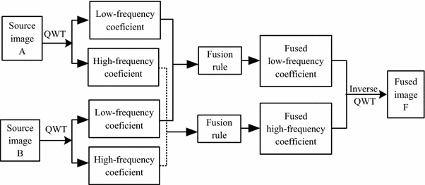

  

  Schematic diagram of proposed fusion method

5 Evaluation Metrics

5.1 Mutual Information

Mutual information (MI), proposed by Piella [24], indicates how much information the fused image conveys about the reference image. MI is defined as $MI = \;MI_{AF} + MI_{BF}$, where $MI_{sF}$ can be calculated as:

$$MI(s;F) = \sum\limits_{u = 1}^{L} {\sum\limits_{v = 1}^{L} {h_{s,F} (u,v)\log_{2} \frac{{h_{s,F} (u,v)}}{{h_{s,F} (u)h_{s,F} (v)}}} }$$

(12)

where s and F denote the source image (A or B) and the fused image, respectively, h _s,F is the joint gray-level histogram of s and F, h _s and h _F are the normalized gray-level histograms of s and F, respectively, and L is the number of bins. A larger MI indicates that the fused image contains more information from images A and B.

5.2 Fusion Performance Characterization

Petrovic proposed an objective image fusion performance characterization [25] based on gradient information to evaluate fused medical images. The metrics are total fusion performance $Q^{AB/F}$, fusion loss $L^{AB/F}$, and modified fusion artifacts $N_{{}}^{AB/F}$ (artificial information created).

The $Q^{AB/F}$ metric considers the amount of edge information transferred from the input images to the fused image. This method uses a Sobel edge detector to calculate the strength and orientation information at each pixel in source images A and B and fused image F. A higher $Q^{AB/F}$ indicates better results. Fusion loss $L^{AB/F}$ can be used to evaluate the information lost during the fusion process (i.e., information available in the source images but not in the fused image). Fusion artifacts $N_{{}}^{AB/F}$ represent visual information introduced into the fused image by the fusion process that has no corresponding features in any of the inputs. The fusion artifacts are essentially false information that directly detracts from the usefulness of the fused image, and can have serious consequences in certain fusion applications. According to [25], a smaller $L^{AB/F}$ indicates better results. Similarly, a smaller $N_{m}^{AB/F}$ meas better results. $Q^{AB/F}$, $L^{AB/F}$, and $N_{{}}^{AB/F}$ are complimentary; i.e., their sum should be unity.

$$Q^{AB/F} { + }L^{AB/F} { + }N_{{}}^{AB/F} = 1$$

(13)

6 Experiments and Discussion

6.1 Experimental Setup

To evaluate the performance of the proposed fusion method, experiments were performed on six pairs of multi-modal medical images, as shown in Fig. 4. To conveniently describe these pairs of images, the images were divided into groups a, b, c, d, e, and f, respectively. In Fig. 4, x1 and x2 ($x \in [a,b,c,d,e,f]$) indicate pairs of source images. Figure 4a1, a2 are a CT image showing bone information and an MRI image showing soft tissue, respectively. Figure 4b1, b2 are a CT image and a proton density (PD)-weighted MR image, respectively. The CT image in Fig. 4c1 and T1-weighted MR-GAD image in Fig. 4c2 show several focal lesions involving the basal ganglia. Figure 4d1, d2 are MRA and T1-weighted MRI images, respectively. Figure 4e1, f1 are T1-MRI images, respectively. Figure 4e2, f2 are T2-MRI images, respectively.

Fig. 4

Source medical images for fusion experiment. a1 CT, a2 MR, b1 CT, b2 PD-weighted MR, c1 CT, c2 T1-weighted MR-GAD, d1 MRA, d2 T1-weighted MR, e1 T1-weighted MR, e2 T2-weighted MR, f1 T1-weighted MR, f2 T2-weighted MR

The performance of the proposed method is compared with the PCNN method motivated by spatial frequency of NSCT coefficients proposed by Xiaobo [26], Sudeb’s method [27] of the PCNN motivated by the modified spatial frequency of NSCT coefficients, the ripplet method [6], and the QWT method based on visibility features proposed by Peng [12]. In Qu’s method and Sudeb’s scheme based on NSCT, the pyramid filter and the direction filter were set to ‘pyrexc’ and ‘vk’, respectively. In Qu’s method, the decomposition levels were set to [0,1,3,3,4]. In Sudeb’s NSCT method, the decomposition levels were set to [1, 2, 4] in accord with [27]. In Sudeb’s ripplet method, the ‘9/7’ filter, ‘pkva’ filter, and levels = [0,1,2,3] were used to decompose the source images using the ripplet transform. In Peng’s method, the parameters given in [12] were adopted for the comparison. For the proposed method, the link range of the PCNN were set as 3, α _L  = 0.06931, α _θ  = 0.2, β = 0.2, V _L  = 1.0, and V _θ  = 20. The maximum number of iterations was set at 200. M = [1.414,1,1.414;0,1,0;1.414,1,1.414]. Two levels of the QWT were adopted.

6.2 Subjective Evaluation Analysis

To evaluate the performance of the proposed method in multi-modal medical image fusion, extensive experiments were performed on the six groups of images shown in Figs. 5, 6 and 7, respectively. From the fusion results of the five algorithms in Fig. 5a–e, all fused images contain both bone information and tissue information. However, careful observation reveals some differences. Figure 5a, b show a block effect and image degradation. There is higher contrast in the fused images obtained using the proposed method and Sudeb’s NSCT method than in those obtained using the other three methods. However, the label regions in Fig. 4e are clearer than those in Fig. 4c.

Fig. 5

Fusion images for groups a and b in Fig. 4 obtained using (a, f) Sudeb’s method (ripplet), b, g Qu’s method, c, h Sudeb’s method (NSCT), d, i Peng’s method, e, j proposed method

Fig. 6

Fusion images for groups c and d in Fig. 4 obtained using (a, f) Sudeb’s method (ripplet), b, g Qu’s method, (c, h) Sudeb’s method (NSCT), d, i Peng’s method, e, j proposed method

Fig. 7

Fusion results for images in Fig. 4e f obtained using (a, f) Sudeb’s method (ripplet), b, g) Qu’s method, c, h Sudeb’s method (NSCT), d, i Peng’s method, e, j proposed method

From Fig. 5f–j, the visual effect in Fig. 5f is the worst. The external outline of Fig. 5g shows some image degradation. Furthermore, the upper outline in Fig. 5h is not as clear as those in Fig. 5i–j. The upper outline of Fig. 5b2 is partly lost in Fig. 5h. However, the corresponding regions are clear in Fig. 5j. The label regions in Fig. 5j are clearer than those in Fig. 5h. The image fused using the proposed method, Fig. 5h, has higher contrast than that in Fig. 5i.

The white outline in Fig. 4c1 is lost in Fig. 6a. There are clear artifacts along the boundary in Fig. 6b. The outline information in Fig. 6e is more obvious than that in Fig. 6c, d. A block effect and artifacts are clearly visible in Fig. 6f, h, and especially in Fig. 6g. The image quality in Fig. 6i, j are similar.

Figure 7a shows that a lot of image information in Fig. 4e1, e2 is lost after the fusion process. Dark blocks appear in the middle part of Fig. 7b. The accuracy and image information in Fig. 7e are better than those in Fig. 7c, d. The lower-right corner of Fig. 7j shows more details of tissues compared to Fig. 7f–i. In summary, the fusion image obtained using the proposed algorithm has more accuracy and necessary information compared to those obtained using the other four methods while having fewer blocks and artifacts.

6.3 Objective Evaluation Analysis

Objective evaluation metrics are used to demonstrate the differences in the fused images. MI, $Q^{AB/F}$, $L^{AB/F}$, and $N^{AB/F}$ are used to compare the proposed method with four algorithms. The objective performances of the fused images of groups a and b in Fig. 4 are listed in Table 1. Table 2 shows the MI, $Q^{AB/F}$, $L^{AB/F}$, and $N^{AB/F}$ values of the fused images in groups c and d in Fig. 4, respectively. Table 3 shows the objective performances of fused images in groups d and e obtained using different methods. The algorithms produces fused images with different objective criteria values. Larger values of MI and $Q^{AB/F}$ and smaller values of L^AB/F and N^AB/F indicate better results. In Tables 1, 2 and 3, the bold values indicate the best results for the four quantitative metrics. The MI and $Q^{AB/F}$ values of the proposed algorithm are the largest for all groups, except for $Q^{AB/F}$ for group c, for which Sudeb’s NSCT method gives the largest value. These results show that the proposed method gives the most useful information in the fused images. The $L^{AB/F}$ values of the fused images obtained using the proposed method are the smallest, except for groups a and c, for which Sudeb’s (NSCT) values are the smallest. The fusion artifact metric, $N^{AB/F}$, values of the proposed scheme are the smallest (i.e., our method introduced the fewest artifacts).

Table 1 Objective evaluation of fusion results for groups a and b

Table 2 Objective evaluation of fusion results for groups c and d

Table 3 Objective evaluation of fusion results for groups e and f

The objective evaluation results well coincide with the subjective effect evaluation with minor exceptions. However, for these exceptions, the subjective effect of the proposed method is better than that of the other methods. From the subjective and objective metric comparisons, it can be concluded that the proposed algorithm works well for combinations of CT with MRI, CT with PD-weighted MR, CT with T1-weighted MR-GAD, MRA and T1-weighted MRI, and T1-weighted MR with T2-weighted MR. The proposed scheme is more effective than some state-of-the-art methods.

7 Conclusion

This study applied the QWT to multi-modal medical image fusion. The proposed method adopts the PCNN fusion rule and abosolute-max fusion rule to select high- and low-frequency coefficients, respectively. The experimental results illustrate that the proposed scheme is better than some existing fusion methods in terms of both objective and subjective metrics.

References

Kettenbach, J., Wong, T. D., Hata, N., Schwartz, R., Black, P., Kikinis, R., et al. (1999). Computer-based imaging and interventional MRI: Applications for neurosurgery. Computerized Medical Imaging and Graphics, 23(5), 245–258.
Zhu, Y. M., & Cochoff, S. M. (2006). An object-oriented framework for medical image registration, fusion, and visualization. Computer Methods and Programs in Biomedicine, 82(3), 258–267.
Wang, L., Li, B., & Tian, L. F. (2014). Multi-modal medical image fusion using the inter-scale and intra-scale dependencies between image shift-invariant shearlet coefficients. Information Fusion, 19(1), 20–28.
Petrovic, V. S., & Xydeas, C. S. (2004). Gradient-based multiresolution image fusion. IEEE Transactions on Image Processing, 13(2), 228–237.
Zhang, X., Zheng, Y., Peng, Y., & Liu, W. (2009). Research on multi-mode medical image fusion algorithm based on wavelet transform and the edge characteristics of images. International Congress on Image and Signal Processing, 1–4.
Das, S., & Kundu, M. K. (2011). Ripplet based multimodality medical image fusion using pulse-coupled neural network and modified spatial frequency. International Conference on Recent Trends in Information Systems, 229–234.
Rajkumar, S., & Kavitha, S. (2010). Redundancy discrete wavelet transform and contourlet transform for multimodality medical image fusion with quantitative analysis. International Conference on Emerging Trends in Engineering and Technology, 134–139. IEEE Computer Society.
Bhatnagar, G., Wu, Q. M. J., & Liu, Z. (2013). Directive contrast based multimodal medical image fusion in NSCT domain. IEEE Transactions on Multimedia, 15(5), 1014–1024.
Wang, Z. (2012). Image fusion by pulse couple neural network with shearlet. Optical Engineering, 51(6), 067005.
Bayro-Corrochano, E. (2006). The theory and use of the quaternion wavelet transform. Journal of Mathematical Imaging & Vision, 24(1), 19–35.
Lam, C. W., Hyeokho, C., & Baraniuk, R. G. (2008). Coherent multiscale image processing using quaternion wavelets. IEEE Transactions on Image Processing, 17(7), 1069–1082.
Peng, G., Xing, S., & Tan, X. (2015). Medical image fusion based on quaternion wavelet transform and visibility feature. International Journal of Applied Mathematics and Machine Learning, 2(1), 9–26.
Yong, Y., Song, T., Shuying, H., & Pan, L. (2014). Log-gabor energy based multimodal medical image fusion in NSCT domain. Computational & Mathematical Methods in Medicine, 2014(1), 835481.
Li, Y., Lu, H., Chen, L., & Serikawa, S. (2015). Medical image fusion using optimal feature selection methods based on second generation contourlet transform. International Journal of Autonomous & Adaptive Communications Systems, 8(2/3), 306–319.
Li, H., Zhang, Y., & Xu, D. (2010). Noise and speckle reduction in doppler blood flow spectrograms using an adaptive pulse-coupled neural network. EURASIP Journal on Advances in Signal Processing, 2010(1), 1–11.
Shang, L., Yi, Z., & Ji, L. (2007). Binary image thinning using autowaves generated by PCNN. Neural Processing Letters, 25(1), 49–62.
Bahri, M., Ashino, R., & Vaillancourt, R. (2011). Two-dimensional quaternion wavelet transform. Applied Mathematics and Computation, 218(1), 10–21.
Yin, M., Liu, W., Shui, J., & Wu, J. (2012). Quaternion wavelet analysis and application in image denoising. Mathematical Problems in Engineering, 2012(1), 587–612.
Yang, S., Wang, M., Lu, Y. X., Qi, W., & Jiao, L. (2009). Fusion of multiparametric sar images based on sw-nonsubsampled contourlet and PCNN. Signal Processing, 89(12), 2596–2608.
Xu, L., Du, J., & Li, Q. (2013). Image fusion based on nonsubsampled contourlet transform and saliency-motivated pulse coupled neural networks. Mathematical Problems in Engineering, 2013(4), 831–842.
Mei-Li, L. I., Yan-Jun, L. I., Wang, H. M., & Zhang, K. (2010). Fusion algorithm of infrared and visible images based on NSCT and PCNN. Opto-Electronic Engineering, 37(6), 90–95.
Wang, Z., & Ma, Y. (2008). Medical image fusion using m-PCNN. Information Fusion, 9(2), 176–185.
Johnson, J. L., Padgett, M. L., & Omidvar, O. (1999). Guest editorial overview of pulse coupled neural network (PCNN) special issue. IEEE Transactions on Neural Networks, 10(3), 461–463.
Piella, G. (2002). A general framework for multiresolution image fusion: From pixels to regions. Information Fusion, 4(4), 259–280.
Petrovic, V., & Xydeas, C. (2005). Objective image fusion performance characterisation. Tenth IEEE International Conference on Computer Vision, 2, 1866–1871.
Xiaobo, Q., Jingwen, Y., Hongzhi, X., & Ziqian, Z. (2008). Image fusion algorithm based on spatial frequency-motivated pulse coupled neural networks in nonsubsampled contourlet transform domain. Acta Automatica Sinica, 34(12), 1508–1514.
Das, S., & Kundu, M. K. (2012). NSCT-based multimodal medical image fusion using pulse-coupled neural network and modified spatial frequency. Medical & Biological Engineering & Computing, 50(10), 1105–1114.
Acknowledgements
The source images used in this paper were downloaded from http://www.med.harvard.edu/aanlib/home.html. This work was supported in part by the National Natural Science Fund under Grants 61572063 and 61401308, the Natural Science Fund of Hebei Province under Grants F2013210094, F2013210109, F2016201187, F2016201142 and Z9904427, and Science research project of Hebei Province under grant QN2016085 and ZC2016040.
Author information
Authors and Affiliations
Corresponding author
Rights and permissions
Open Access This article is licensed under a Creative Commons Attribution 4.0 International License, which permits use, sharing, adaptation, distribution and reproduction in any medium or format, as long as you give appropriate credit to the original author(s) and the source, provide a link to the Creative Commons licence, and indicate if changes were made.
The images or other third party material in this article are included in the article’s Creative Commons licence, unless indicated otherwise in a credit line to the material. If material is not included in the article’s Creative Commons licence and your intended use is not permitted by statutory regulation or exceeds the permitted use, you will need to obtain permission directly from the copyright holder.
To view a copy of this licence, visit https://creativecommons.org/licenses/by/4.0/.
About this article
Cite this article
Geng, P., Sun, X. & Liu, J. Adopting Quaternion Wavelet Transform to Fuse Multi-Modal Medical Images. J. Med. Biol. Eng. 37, 230–239 (2017). https://doi.org/10.1007/s40846-016-0200-6
Received:
Accepted:
Published:
Issue Date:
DOI: https://doi.org/10.1007/s40846-016-0200-6