The Influence of the R-Phase on the Superelastic Behavior of NiTi

Abstract

Approximately equiatomic Ni–Ti alloys, or Nitinol, can transform upon cooling or when stressed from a parent ordered cubic (B2) Austenite phase into two martensitic structures: a monoclinic structure commonly referred to as simply martensite and a rhombohedrally distorted martensite referred to as the R-phase. While the former is often more stable, the R-phase presents a substantially lower barrier to formation, creating an interesting competition for the succession of Austenite. This competition has markedly different outcomes depending upon whether Austenite instability is caused by cooling or by the application of stress. While medical applications are generally used isothermally, most characterization is done using thermal scans such as differential scanning calorimetry. This leads to frequent and significant misunderstandings regarding plateau stresses in particular. The purpose of this paper is to discuss the competition between these two martensites as the parent Austenite phase loses stability, and to clarify how tests can be properly conducted and interpreted to avoid confusion. To that end, the examples shown are not selected to be ideal or theoretical, but rather to illustrate complexities typical of those found in medical devices, such as cold worked conditions that make peaks difficult to interpret and “plateaus” ill-defined. Finally, a stress-induced M ⇒ R ⇒ M sequence will be discussed.

Background

Otsuka et al. [1] provides a clever metaphor relating Austenite as it is cooled to an unpopular and unstable government. As dissatisfaction with an extant government rises, there are signs of instability: demonstrations and skirmishes such as the Boston Tea Party. Before there is organized rebellion, there are transient signs that the current regime is becoming unstable. Eventually, skirmishes become organized, war breaks out, and the existing regime is overthrown. But rebellions are a complaint against the current regime more than an effort to install any particular new form of government. Once the reigning government is overthrown, a new governing structure must be installed. Often, a make-shift, interim government is installed—one that is easily and quickly formed but will later have to be replaced by more stable structure. Such was the case with both the American and French revolutions.

By metaphor, nature seeks ordered, lower entropy structures as temperature is reduced. The relatively high entropy of the cubic Austenite structure of Ni–Ti causes an energetic dissatisfaction: as Austenite is cooled, one begins to see evidence of instability, such as a pronounced reduction in Young’s modulus (lattice softening). With further cooling, the Austenite phase gives way. Ni–Ti offers two candidate successors of lower entropy, a monoclinic B19′ martensite and a rhombohedrally distorted martensite (the R-phase). To avoid confusion, we will distinguish the two martensitic products by referring to them as M and R, respectively. Whether it is the M or R structure that replaces Austenite depends on both thermodynamic and kinetic factors. Often M is thermodynamically preferred, but R is initially formed because it is kinetically advantaged, presenting a lower activation energy.

Most engineers working with Nitinol are familiar with the monoclinic martensite (M) but less so with R. Several excellent reviews of the R-phase exist [1–3], but the present discussion is less about the phases themselves than it is about the competition between the two, making an intimate knowledge of R is unnecessary. Still, several summary points are essential to this paper’s objectives:

• 1. The R-phase can be imagined as a rhombohedral distortion of the cubic austenitic phase (Fig. 1), with one of the four [1 1 1] directions of the cubic Austenite stretched. Figure 1 deliberately avoids depicting atoms—atomic shuffles do accompany the transformation making the actual structure significantly more complicated [4, 5] but our interests lie in the distortion rather than the crystallography.

  Fig. 1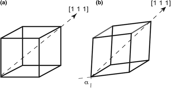

  

  The distortion from the cubic austenitic phase (a) to the R-phase (b) creates a rhombohedral distortion, lengthening one of the four [1 1 1] directions and leaving all three angles α slightly equal but less than 90°. As the rhombohedral angle contracts, the distortional strain in the [1 1 1] direction increases

• 2. The M-phase can be imagined as a monoclinic distortion of the cubic austenitic phase (Fig. 2) with an unequal stretch along two perpendicular (1 1 0) directions followed by a change in the angle between [1 1 0] and [0 0 1].

  Fig. 2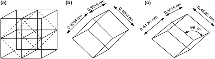

  

  The M distortion can be envisioned by a imagining four austenitic cells, b redefining the austenitic cell as a tetragonal cell, and c stretching one cell edge, compressing a second, and distorting one angle, as shown in (c)

• 3. Both the A ⇒ R and A ⇒ M transformations are martensitic and are easily reversed by heating (A ⇔ M and A ⇔ R). Further, both introduce very small volume changes and can be self-accommodated by combining twin-related variants. Both transformations are thermoelastic and have all the typical characteristics of a shape memory alloy, including shape memory and superelasticity.

• 4. The uniaxial tensile transformational strain (ε _t) associated with A ⇔ M is 6–7 % in typically textured superelastic Nitinol, while the transformational strain of the A ⇔ R transformation is only on the order of 0.2–0.5 %.

• 5. With respect to the above point, the transformational strain of the A ⇔ R transformation is not fixed: the rhombohedral angle, α, continues to contract as the R-phase is cooled. This second order increase in ε _t is interrupted if and when M takes over, but if one suppresses M and maintains the stability of R to very low temperatures, transformational strains as high as 1.5 % can be achieved [2, 6, 7].

• 6. Twin boundaries in both M and R are highly mobile, but it is substantially easier to move twins in R than in M. Thus, yield stresses for M are typically 200–250 MPa, while those of R are 5–25 MPa. Similarly, the thermal hysteresis of R is much less than M: 1–5 °C for A ⇔ R versus 30–50 °C for the A ⇔ M transformation.

• 7. Because both the A ⇔ R and the A ⇔ M transformations are thermoelastic, they both individually follow the Clausius–Clapeyron equation:

$${\text{d}}\sigma /{\text{d}}T \, = \Delta H \, / \, T\varepsilon_{\text{t}}$$

(1)

• 8. The latent heats of transformation for the two transformations (ΔH) are similar, as will be demonstrated later. Because ε _t is so much smaller for A ⇔ R, the stress rate, dσ/dT, is far greater.

• 9. In addition to the A ⇔ R and the A ⇔ M transformations, one can also reversibly transform between the two candidate successors (R ⇔ M). For example, R can form first, but when further cooling increases the thermodynamic preference for M, kinetic barriers are eventually overcome and M will replace R.

• 10. The R ⇔ M transformation also follows the Clausius–Clapeyron equation, with similar parameters to that of the A ⇔ M transformation, though with slightly reduced transformational strains. The kinetic barriers to forming M from R are also similar to those of forming M from A (a similar hysteresis, for example).

With this summary, the following section will discuss the effect of temperature on the competition for succession, and the next to the effect of stress in the next section.

The Effect of Temperature on the Competition Between M and R

In this section, the effects of temperature on the three phases, A, M, and R will be discussed, the assumption being that there are no stresses that might impact their relative stability.

Based on the above nine points, one can envision four scenarios for the succession of Austenite as it loses stability during cooling and reverts during subsequent heating.

• 1. The direct transformation to M (A ⇒ M on cooling and M ⇒ A on heating). In this simplest of scenarios, M is more stable than R at all temperatures, and the kinetic advantages of R are insufficient to overcome the energetic advantages of M. R never enters the picture. While this is common in fully annealed alloys, and is the sequence most frequently assumed in the literature, it is rarely observed in medical devices.

• 2. The direct transformation to R (A ⇒ R on cooling and R ⇒ A on heating). Certain ternary additions, such as Fe, Co, and Cr suppress M resulting in alloys that form R upon cooling, but do not form M without the application of a stress. While again not pertinent to medical devices, it is included for the sake of completeness.

• 3. The symmetric R-phase transformation (A ⇒ R ⇒ M on cooling and M ⇒ R ⇒ A on heating). In this case, there is a temperature window in which R is thermodynamically favored over both A and M. Since the barriers to forming R are also less than for M, R appears in both the forward and reverse directions, intermediate to A and M.

• 4. The asymmetric R-phase transformation (A ⇒ R ⇒ M on cooling and M ⇒ A on heating). In this case, M is energetically preferred over R at all temperatures, but the lower kinetic barriers to R formation permit it to form on cooling before M takes over. Upon heating, however, the kinetic barriers to forming A are overcome before M can form R.

In the cold worked and aged nickel rich alloys most commonly used for medical devices, one seldom if ever finds the first or second scenarios, but both the symmetric and asymmetric scenarios are commonplace and thus become the focus here. As will be shown, the difference is critical to how one interprets transformation temperatures.

Figure 3 schematically portrays the symmetric R-phase transformation. Figure 3(a) depicts a schematic free energy diagram for the three phases. The entropy of R (the slope of the free energy curve) is intermediate to that of A and M, as one expects given the crystallographic symmetries of the competing phases. Of note, there is a temperature regime during which each of the three phases is thermodynamically most favorable. The formation of M from either A or R, however, presents a larger kinetic barrier than does A or R. The more difficult kinetics involved in formation and reversion of M results in a greater thermal range for R stability during cooling.

Fig. 3

In the symmetric transformation, each of the three phases is the most stable at some temperature and the R-phase is observed in both cooling and heating. a schematic of the free energy curves with the black dotted line illustrating the path taken during cooling and subsequent heating is shown in (1). Figures b and c, respectively, map idealized corresponding transformational strains and DSC curves. Not kinetic facility of forming R from A creates a much broader range for R on cooling than upon heating

In Fig. 3(b), the transformational strain is conceptually portrayed. The word “conceptually” is used in the previous sentence because the temperature at which shape changes during cooling can only be measured with a stress applied, which of course shifts the transformation temperatures. Note the three stages during cooling: (1) the first order transformation from A to R, (2) a continuous exaggeration of the rhombohedral distortion as discussed above, and finally (3) the replacement of R with M. The three segments are reversed on heating.

Figure 3(c) shows the heat released and absorbed as the transformations occur, with two distinct and approximately equal peaks during heating and cooling as would be produced by differential scanning calorimetry (DSC).

Figure 4 treats the asymmetric transformation in the same manner. In Fig. 4(a) shows that R is never the lowest energy phase. It appears on cooling only because the kinetic barrier to forming R is lower than to form M: the A ⇒ R transformation provides temporary respite until supercooling is sufficient to form M. On heating, however, A forms before R becomes more stable than M. Figure 4b, c shows two stages/peaks during cooling, but direct transformation from M to A on heating.

Fig. 4

In the asymmetric transformation the R-phase is never the most phase, but is still formed upon cooling due to its lower kinetic barrier

To exemplify these principles, we examine a 0.5-mm diameter wire made from binary Nitinol with a nickel content of 50.8 atomic percent; more titanium is tied up in oxides and carbides than is nickel, so the composition of the actual NiTi compound is approximately 51.0 %.¹ The wire was cold worked 40 % and strand annealed at a temperature and stress sufficient to straighten the wire but that preserved substantial cold work, typical of materials used to make medical devices.

Figure 5 shows a DSC curve of the wire as it might be heat treated to make a stent: 500 °C for 10 min. Two peaks are labeled on the figure upon cooling (A ⇒ R and R ⇒ M) and two peaks upon heating (M ⇒ R and R ⇒ A), thus we have a symmetric transformation through the R-phase. For reference, the dotted trace in Fig. 5 is the DSC response prior to the heat treatment.

Fig. 5

DSC trace of 50.8 at% wire is shown as drawn and straightened (dotted line) and after a typical heat treatment, at 500 °C for 10 min. Both show four peaks (a symmetric transformation), though the R ⇒ M is ill-defined in the as-straightened wire

The wire was also heat treated at 325 °C for 100 min in order to separate the R and M transformations and allow a clearer examination of their competition. The DSC trace is shown in Fig. 6, but this time ASTM’s transformation temperature definitions [8] have been added. The R ⇒ M peak is broad and unconvincing, which prevented the identification of peak specifics (M _s, M _p and M _f). In fact, the broad bump that appears during cooling looks similar to the testing anomaly occurring just after the heating cycle begins. It is very common to “lose” this second cooling peak when the test subject is a colder alloy with substantial retained cold work. Still, there must be an R ⇒ M transformation during cooling or there could not be two peaks upon heating—M must form before it can revert. To demonstrate this, Fig. 7a shows DSC heating traces after cooling to various temperatures. Figure 7b shows an integration of the peaks, nicely defining the M _s to M _f transformational range, even though the R ⇒ M peak itself cannot be distinctly found.

Fig. 6

DSC trace of the as-straightened wire after heat treating for 100 min at 325 °C. The definitions added to the figure are drawn from ASTM F 2005—05 [7]

Fig. 7

a shows the heating trace of DSC tests that were initially cooled to the temperature shown in the legend. b shows the integral of the M ⇒ R peak showing when M was formed during cooling

The above highlights one of most frequent and dangerous pitfalls of DSC interpretation: investigators often do not cool far enough to form M, and as a result, obtain only one cooling and one heating peak, neither of which pertains in any way to M. This leads to misinterpretation and misuse of the A _f temperature. If one observes two peaks (one in each direction), one knows at a glance whether they are due to the A ⇔ R transformation based on the small hysteresis (under ten degrees).

Finally, from a practical perspective, one must be aware that there are other unusual circumstances that could give rise to four peaks: certain ternary alloys containing copper [9] and certain aging conditions that result in inhomogeneity [10–12] can also produce extra peaks. These are not the subject of this paper, but four peaks due to a symmetric R-phase transformation is uniquely characterized by the large disparity in peak spacing between cooling and heating.

Figure 8 shows the Bend Free Recovery (BFR) behavior of the same wire as that used in Figs. 6 and 7. The wire was tested per the BFR ASTM standard [13] after an outer fiber strain of 3 %. The bulk of the recovery is commensurate with the reversion of M, as expected, and corresponds to the M ⇒ R in the DSC traces. The R ⇒ A peak correlates to the small recovery at the end of the heating. Figure 8 also highlights the second order modification of the rhombohederal angle of R.

Fig. 8

Typical bend-free recovery test indicative of a symmetric transformation, labeled per the ASTM specification [10]

The DSC and BFR results are summarized in Table I. The agreement is generally good, given the substantial challenges presented in drawing tangents and baselines, particularly since the M ⇒ R does not complete before the onset of the R ⇒ A transformation. All the tests were repeated several times and are reproducible to within 2 °C.

Table I Transformation temperatures after heat treating 325 °C for 100 Min

The Effect of Stress on the Competition Between Phases

By and large, medical devices operate isothermally at 37 °C and the competition for Austenite succession is controlled by stress rather than temperature. While related, the outcomes are quite different.

As discussed in “Background” section, all the transformations of concern (A ⇔ M, A ⇔ R, and R ⇔ M) obey the Clausius–Clapeyron equation, though the stress rate, dσ/dT, is dramatically higher for A ⇔ R because the transformational strains are markedly less. In short, stress has a much lesser effect on the stability of R than it does on M. While one can stress induce R, it can only be done over a narrow temperature range—much narrower than one can stress induce M. Looking at this from another perspective, if it were practical to perform the DSC test shown in Fig. 5 under stress, one would find that as stress increases, the R ⇒ M and M ⇒ R peaks would rapidly move to higher temperatures and soon overtake and eliminate peaks associated with the A ⇒ R and R ⇒ A transformations, resulting in the direct A ⇔ M transformation.

To exemplify this, the same wire that was measured in Fig. 6 through Fig. 8 was tensile tested at a variety of temperatures. Water was used to control temperature and avoid adiabatic heating. Figure 9 shows a composite of loading and unloading curves at various temperatures, focusing on the 0–3 % strain range where the M/R competition manifests. Before delving into the detail of this figure, a few comments regarding the experimental approach are in order. The tests were run sequentially, from the warmest to coolest test temperature, using the same specimen—that very same specimen was later used to create Fig. 6. Because many of the tests exhibited a small amount of thermally recoverable residual set, the wire was warmed to 50 °C between each test to fully recover the original shape (this will be discussed more later). Finally, prior to the test sequence, the wire was run though one superelastic cycle to 6 % strain at 37 °C in order to better simulate what a typical medical device might experience (devices are typically crimped, deployed then implanted).

Fig. 9

Tensile tests performed in water at various temperatures

Our examination of Fig. 9 will cover two distinct and different subjects: first the flat loading and unloading plateau, and second the yielding phenomenon that obviously markedly changes with temperature.

The plateaus, loading, and unloading are due to the transformation to M and the subsequent reversion of M, respectively. It is not important whether M is forming from A or R, or whether it reverts to R or A. If the temperature at which M reverts without stress is tentatively labeled M _R, then the unloading plateau should be:

$$\sigma_{\text{LP}} = {\text{ d}}\sigma /{\text{d}}T \, (T_{\text{o}} {-} \, M_{\text{R}} )$$

(2)

where σ _LP is the lower plateau stress and T _o the ambient test temperature. Where many are confused is in relating M _R to the features on a DSC or BFR test. Notably, M _R becomes the A _p temperature when the transformation from M ⇒ A is direct, but R′_p when the transformation proceeds M ⇒ R ⇒ A. This is a serious deficiency in the current terminology of our industry. In short, the A _f and A _p temperature are not relevant to the plateaus of this alloy, nor of other typical medical device material, rather it is the M ⇒ R peak that defines superelasticity and R′_p that should be inserted as M _R in Eq. 2.

To demonstrate this point, Fig. 10 maps the plateau stresses of Fig. 9 as a function of test temperature. The unloading point extrapolates to zero at 5 °C, consistent with the DSC and BFR results for M ⇒ R, but not R ⇒ A. The unloading plateau in Fig. 9 disappears entirely at 5 °C in perfect agreement with the ASTM-defined R′_f.

Fig. 10

Upper and lower plateau stresses in Fig. 9 versus test temperature. Plateaus are measured at 2.5 % strain

If one attempts to apply the same equation to the loading plateau, the fit is poor. In this case, the loading plateau extrapolates to zero at −65 °C, well above the entire R ⇒ M range derived by Fig. 7b. To extrapolate to the peak temperature, dσ/dT would have to be 3.0 MPa/ °C rather than the measured 4.6 MPa/ °C. This is not surprising given that ε _t for R increases with cooling—the linearity assumption fails.

The next topic of discussion is the yielding phenomena in Fig. 9. According to Fig. 6, R should be present at the onset of testing below approximately 30–40 °C, meaning that M will be stress induced from R rather than A. Prior to stress inducing M, however, the R itself twins, and does so at very low stresses—essentially at the very onset of loading. (A slight inflection is present in Fig. 9 loading, but it is too weak to be discerned without very careful analysis—annealing, or using fresh wires increase the plateau definition.)

During unloading, M reverts to R, but that reversion occurs under stress and therefore to the deformed variants rather than the self-accommodating variants. Heating will fully recover that deformation, but mapping the residual strain, prior to heating is a useful way of studying the transformational strain of R (Fig. 11). Agreement with the A ⇒ R peak in Fig. 6 is excellent: the greater the fraction of R present at the start of the test, the greater the residual set at the end of the test, and the colder the test temperature, the greater is ε _t.

Fig. 11

Residual set after unloading as a function of temperatures. These strains are fully recovered by heating to 50 °C

Above 30 °C, Fig. 6 indicates the starting condition is primarily Austenite, but R is stress induced before M is formed. It rapidly becomes more difficult to stress induce R as temperature is increased (the high dσ/dT). At 50 °C, M is directly stress induced from A—there is no trace of R. One can estimate the stress rate of the A ⇒ R transformation by determining the stress at which the slope increases from that resulting from R twinning to that of the elastic loading of R, determined by taking the derivative of the loading curves. While somewhat ill-defined, the results (Fig. 12) indicate a stress rate of approximately 16 MPa/ °C. This should not, however, be a straight line due to the ever-increasing rhombohedral distortion.

Fig. 12

R-Phase inflection point versus temperature

To summarize:

• It is the reversion of M that controls the unloading plateau, not necessarily the formation of Austenite.

• In most medical devices, M reverts to R, so there is no correlation between A _f and lower plateau stress. Correlation is always to the first peak encountered during heating, be that to R or A.

• While R is often prominent during thermal testing, it is usually absent at body temperature. At body temperature M is generally directly stress induced.

The M ⇒ R ⇒ M Transformation

While perhaps counterintuitive, one can also stress induce R from M even though M is more stable under stress. At low temperatures where M is the incumbent structure, the application of small stress may be insufficient to move the twin boundaries of M but sufficient to move R twins. In this case, strain energy can be reduced by stress inducing R. As the R transformational strain is reached, stress again increases and M eventually replaces R. In other words, the transformation sequence is: M ⇒ R ⇒ M. An example is shown in Fig. 13. Here, the same wire condition is tested at −40 °C, in one case with R the starting phase, in the other with M the incumbent (differentiated based on whether the wire is cooled or heated to −40 °C). In both cases, there is a distinct R plateau prior to forming M. It is not clear why the stress needed to induce M is somewhat different in the two cases.

Fig. 13

The same wire condition as shown in Fig. 6 (with no pre-strain) is tested at −40 °C, but in one case cooled to −40 °C so as to make the starting condition R, and in the other case, heated from −196 °C to −40 °C so that the starting condition is M. Both conditions show a distinct R plateau before stress inducing M

Conclusions

To illustrate the above principles, two medical devices will be briefly considered: a typical stent and a guidewire.

• In the case of a stent made from the alloy heat treated as shown in Fig. 5, crimping into a catheter at or below room temperature will cause M to be stress induced from R and the force will be controlled by the difference in temperature between the R ⇒ M peak and the crimping temperature. The stent remains M until deployed at body temperature. Since R is not stable at body temperature, the reversion upon deployment is from M ⇒ A, yet the force against the vessel wall (Chronic Outward Force) is controlled by the M ⇒ R DSC peak (called R′_f in the ASTM standard). The only importance of A _f is to assure that the ultimate diameter is achieved at body temperature—to prevent the residual set shown in Fig. 11.

• Guidewire performance depends upon “stiffness,” but there are two stiffnesses of relevance: the modulus of at the very onset of loading and the plateau stress. Here, one cares about both the R peak (to stiffen the initial loading) and the M peak to increase the plateau stresses. But this is superficial: bench tests to evaluate the initial loading stiffness are often performed on perfectly straight wires where the R is present. In even a mildly tortuous anatomy, however, the strains are well beyond the scope of R and are more likely to be dictated by M.

The above raises important issues pertaining to the terminology used by our industry. A _f, as defined by the literature and ASTM, could mean the temperature at which R reverts, or that M reverts and the two have very different implications. Moreover, it is perfect possible to move the M and R reversion peaks independently by tailoring heat treatment times and temperatures. There is a clear need to modify our terminology so that parameters have the same meaning regardless of the transformational sequence, and so that engineers need not study papers such as this to control their products. Pending such reclassification, it is recommended one is cautious and refers to M _r, the M reversion temperature, ambiguous with respect to whether that is A _f or R′_f.

References

Otsuka K, Ren X (1999) Physical metallurgy of Ti-Ni-based shape memory alloys. Intermetallics 7:511
Ling HC, Kaplow R (1981) Stress-induced shape changes and shape memory in the R and martensite transformations in equiatomic NiTi. Metall Trans 12A:2101
Miyazaki S, Otsuka K (1986) Deformation and transformation behavior associated with the R-phase in Ti-Ni alloys. Metall Trans A 17:53–63
Sitepu H (2003) Use of synchrotron diffraction data for describing crystal structure and crystallographic phase analysis of R-Phase NiTi shape memory alloy. Textures Microstruct 35(3/4):185
Khalil-Allafi J, Schmahl WW, Toebbens DM (2006) Space group and crystal structure of the r-phase in binary NiTi shape memory alloys. Acta Metall 54:3171
Proft JL, Duerig TW, Melton KN (1987) Yield drop and snap action in a warm worked Ni-Ti-Fe alloy. ICOMAT-86 (Jpn Inst Metal) p 742
Miyazaki S, Kimra S, Otsuka K (1988) Shape-memory effect and pseudoelasticity associated with the R-phase transition in Ti-50.0 at.%Ni Single Crystals. Phil Mag A 57(3):467
ASTM F 2005—05, Standard Terminology for nickel-titanium shape memory alloys
Frenzel J, Wieczorek A, Opahle I, Maa B, Drautz R, Eggeler G (2015) On the effect of alloy composition on martensite start temperatures and latent heats in Ni–Ti-based shape memory alloys. Acta Mater 90:213–231
Eggeler G, Allafi JK, Dlouhy A, Ren X (2003) On the role of chemical and microstructural heterogeneities in multistage martensitic transformations. J Phys IV Fr 112:673
Schryvers D, Tirry W, Yang ZQ (2006) Measuring strain fields and concentration gradients arount Ni4Ti3 precipitates. Mater Sci Eng A 438–440:485
Fan G, Chen W, Yany W, Zhu J, Ren X, Otsuka K (2004) Origin of abnormal multi-stage martensitic transformation behavior in aged Ni-rich Ti-Ni shape memory alloy. Acta Mater 52:4351–4362
ASTM F 2082—06, Standard test method for determination of transformation temperature of nickel-titanium shape memory alloys by bend and free recovery
Author information
Authors and Affiliations
Corresponding author
Rights and permissions
About this article
Cite this article
Duerig, T.W., Bhattacharya, K. The Influence of the R-Phase on the Superelastic Behavior of NiTi. Shap. Mem. Superelasticity 1, 153–161 (2015). https://doi.org/10.1007/s40830-015-0013-4
Published:
Issue Date:
DOI: https://doi.org/10.1007/s40830-015-0013-4