
Abstract
Oil transport is greatly affected by heterogeneous pore–throat structures present in shale. It is therefore very important to accurately characterize pore–throat structures. Additionally, it remains unclear how pore–throat structures affect oil transport capacity. In this paper, using finite element (FE) simulation and mathematical modeling, we calculated the hydrodynamic resistance for four pore–throat structure. In addition, the influence of pore throat structure on shale oil permeability is analyzed. According to the results, the hydrodynamic resistance of different pore throat structures can vary by 300%. The contribution of additional resistance caused by streamline bending is also in excess of 40%, even without slip length. Furthermore, Pore–throat structures can affect apparent permeability by more than 60% on the REV scale, and this influence increases with heterogeneity of pore size distribution, organic matter content, and organic matter number. Clearly, modeling shale oil flow requires consideration of porous–throat structure and additional resistance, otherwise oil recovery and flow capacity may be overestimated.
1 Introduction
Shale oil plays a growing role in the global energy supply chain as conventional oil reserves decline. The existence of numerous pore–throat structures in shale reservoirs causes a continuous alteration in the flow path’s width during the flow of shale oil (Wang et al. 2023; Nelson 2009; Su et al. 2022; Chauhan et al. 2021). Consequently, it is essential to investigate pore–throat structures and their impact on shale oil flow (Tan et al. 2022).
The primary reason for the existence of pore–throat structures in shale is its high heterogeneity (Cai et al. 2018). Shale consists of various inorganic mineral components, such as quartz, calcite, dolomite, and organic matter (Gupta et al. 2017, 2018; Xu et al. 2022; Hu et al. 2023; Sun et al. 2023a, b). The different shapes of each component particle result in interparticle pores having pore–throat structures. For example, Naraghi et al. (2018) found by SEM that feldspar, calcite, and clay in shale are elliptical, while quartz is pentagonal. Moreover, pore size is multiscale in shale reservoirs (Taghavinejad et al. 2021; Chen et al. 2021; Sun et al. 2022). For organic matrix, the pore size ranges from 10 to 500nm, while for inorganic matrix, it ranges from 10 nm to 100 mm (Naragh and Javadpour 2015; Clarkson et al. 2013). Furthermore, micro-fractures and fractures produced by hydraulic fracturing are much larger (Li et al. 2022; Xu et al. 2019). Consequently, the flow path size often changes abruptly when fluids flow between OM and iOM or from pores to fractures (Lee et al. 2016).
In order to facilitate theoretical research, many researchers used simplified regular shapes to represent pore–throats, which can be divided into two categories: (1) Pore throats that abruptly change in size or flow direction. (2) Pore throats that gradually change in size or flow direction. The size of type (1) can be characterized by piecewise function (Gravelle et al. 2013; Li et al. 2019; Chao et al. 2019), as shown in structure IV in Fig. 1. Type (2) can be represented by a variety of mathematical functions and is widely used for mathematical modeling, as shown in structures I, II and III in Fig. 1. Cai et al. (2019) and Müller-Huber et al. (2016) used exponential function (I in Fig. 1) to characterize pore–throat structure and calculated permeability of porous media. Sinha et al. (2013) and Fyhn et al. (2021) used trigonometric functions (II in Fig. 1) to study the immiscible two-phase flow in single capillary and porous media, respectively. Besides, in microfluidic experiments (Xu et al. 2017) and pore network models (Suh and Yun 2018), channels composed of circular particles (III in Fig. 1) are often used to represent pore–throat structures.

Pore–throat structures of shale oil flow and its mathematical approximation
Experiments, numerical simulations and mathematical model calculations show that the pore–throat structures have many complex characteristics compared with the constant-radius pore. Li et al. (2019) found that flow pattern transformations in viscoelasticity fluids are greatly influenced by the pore–throat structures. The molecular simulation results of Lee et al. (2016), Zhang et al.(2020) and Sun et al. (2022) found that hydrocarbon fluids will encounter an energy barrier in pore–throat structures. In addition, due to the bending of the streamline, an additional hydrodynamic resistance called the entrance effect will generate when flowing through the pore–throat structures (Gravelle, et al. 2013). Sampson (1891) first derived the pressure drop caused by the entrance effect of liquid transport through a circular hole in an infinite film. Then Dagan et al. (1982) extended the result to convergent flow into a cylindrical pore. Based on FE simulations, Gravelle et al. (2013) modified Sampson’s model to allow it to calculate the additional hydrodynamic resistance of the right part of structure IV in Fig. 1. Wang et al. (2019a, b) then applied it to structure II in Fig. 1 to calculate the entrance effect. While studies have investigated the influence of hydrodynamic resistance on shale oil flow in a single pore–throat structure, the differences in hydrodynamic resistance between structures I, II, III and IV (Fig. 1) have not been extensively studied yet, and the effect of additional resistance generated by different pore–throat structures on permeability has not been fully understood.
In this work, FE models of four pore–throat structures were constructed to calculate the total hydrodynamic resistance in Sect. 2.1. Then in Sect. 2.2, based on Gravelle’s model, the resistance caused by inner effect and entrance effect were derived and fitted by FE results. In Sect. 2.3, we constructed the permeability model coupling pore–throat structures on a REV scale. Finally, the effects of pore–throat structures on permeability with different pore sizes, OM content and distribution were discussed.
2 Methodology
2.1 Finite element model of pore–throat structures
Based on previous research, four pore–throat structures were used in this work, as shown in Fig. 2. Structure I can be expressed as (Cai et al. 2019):
where, \(r_{{\text{t}}}\) is the pore–throat radius, nm; \(\alpha = \frac{{\ln \left( {r_{\max } /r_{\min } } \right)}}{{L_{{\text{t}}} }}\); \(L_{{\text{t}}}\) is the pore–throat length, nm.

Four pore–throat structures constructed in this work. The structures have same rmin, rmax and Lt
Structure II is (Wang et al. 2019a, b):
where \(a = \frac{{r_{\max } - r_{\min } }}{2}\), \(b = \frac{1}{{L_{{\text{t}}} }}\), \(c = \frac{{r_{\max } + r_{\min } }}{2}\).
Structure III can be written as:
where \(R = \frac{{r_{\max } - r_{\min } }}{2} + \frac{{L_{{\text{t}}}^{2} }}{{2\left( {r_{\max } - r_{\min } } \right)}}\) is the circle radius; \(\beta = \frac{{r_{\max } + r_{\min } }}{2} + \frac{{L_{{\text{t}}}^{2} }}{{2\left( {r_{\max } - r_{\min } } \right)}}\). To avoid \(r_{\max } > r_{\min } + R\), structure III should meet:
The part with varying radius of structure IV can be expressed as:
It should be noted that the entrance effect only occurs at the corner (Gravelle et al. 2013). It is therefore necessary to have a part with a constant radius \(r_{\min }\).
To calculate the total hydrodynamic resistance of the four structures, 2D FE models (COMSOL 3.5) were established, as shown in Fig. 3. Table 1 lists fixed parameters used in FE models. In addition, the Navier slip condition was used to characterize widespread velocity slip in shale nanopores (Wang et al. 2019a, b).

The velocity distribution of four pore–throat structures obtained by FE simulations (COMSOL 3.5). Blue represents the minimum velocity, while red represents the maximum velocity
By analogy with Ohm’s law, hydrodynamic resistance is defined as:
where, Rt is the total hydrodynamic resistance, mPa s/nm2; Q is the flow flux, nm2/s; ΔP is the pressure difference, Pa. between the inlet and outlet for structure I, II, and III, while for structure IV is the pressure difference between x = Lp and outlet.
2.2 Mathematical model of pore–throat structures
Based on the N–S equation and considering the Navier slip condition, the flow flux of a 2D pore with a constant radius is expressed as:
where, Qslip-p is the flow flux considering velocity slip, nm2/s; η is the oil viscosity, mPa s; Lp is the pore length, nm; ls is the slip length, nm; rp is the pore radius, nm. Then, the hydrodynamic resistance can be written as:
where the Rslip-p is defined as inner hydrodynamic resistance. For the four pore–throat structures with different radius, the resistance can be expressed as
For the hydrodynamic resistance caused by the entrance effect, Gravelle et al. (2013) gave an empirical formula in 3D structure IV:
where Cr is a numerical prefactor; θ is the angle between the pore wall’s tangent and horizontal direction. Here, we tried to use Eq. (10) to describe the Rent of structure IV:
Because the θ of structure I, II and III change with x, the Rent should be expressed as:
The Maclaurin expansion of sin(dθ) is:
The higher order infinitesimal term of dθ is ignored, and Eq. (13) can be simplified as follows:
where \(\theta\) can be calculated by:
Combing with Eqs. (1–5) and (14–15), the Rent of structure I–IV can be obtained.
Structure I:
Structure II:
Structure III:
Structure IV:
2.3 Apparent permeability model of shale oil
The main characteristics of shale different from traditional reservoirs are: (1) Containing OM, (2) Rich in nanopores, and (3) Different pore size distributions (PSDs) in OM and iOM (Wood 2021). Therefore, to study how the content and distribution of OM and the PSD affect the influence of pore–throat structures on permeability, we use the model established in previous work (Xu et al. 2021). Table 2 lists the basic parameters used, and below are the steps to follow:
-
(1)
Using Quartet Structure Generation Set (QSGS) algorithm (Wang et al. 2007) to construct the 2D spatial distribution model of iOM and OM. As shown in Fig. 4 a, the OM (red part) are randomly distributed in iOM (blue part).
Fig. 4 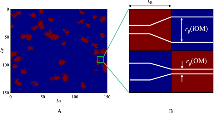
Spatial distribution model of OM and iOM. a Red represents OM and blue represents iOM b Constructing pore–throat structures between adjacent grids, red represents OM grids and blue represents iOM grids
-
(2)
Assigning pore size to each grid. In this work, PSDs of OM and iOM were characterized using logarithmic normal distributions, i.e. (Zhang et al. 2019):
$$f\left( {r_{{\text{p}}} } \right) = \frac{\Delta p}{{r_{{\text{p}}} \sqrt {2\uppi } \sigma }}\exp \left[ { - \frac{1}{2}\left( {\frac{{\ln r_{{\text{p}}} - \mu }}{\sigma }} \right)^{2} } \right]$$(20)where σ is the logarithmic standard deviation; μ is the logarithmic mean. Based on Eq. (20), the pore size of each grid was set by Monte Carlo sampling method.
-
(3)
Connecting adjacent grids with pore–throat structures (Fig. 5b).
Fig. 5 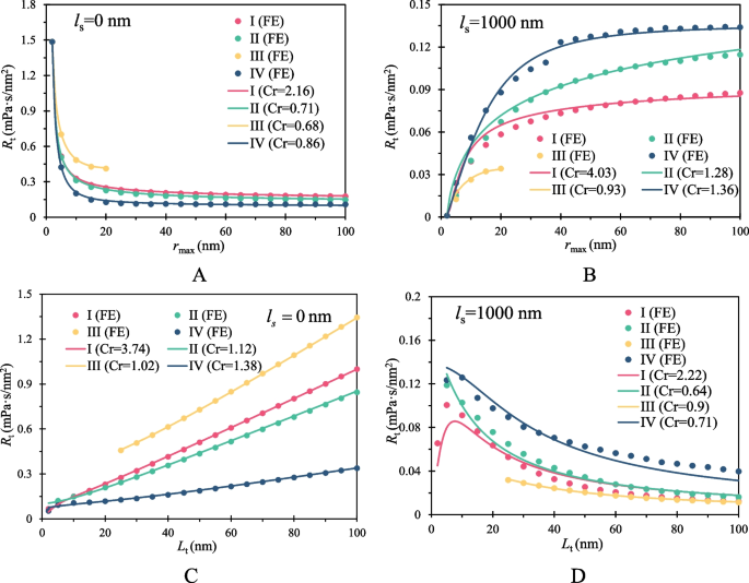
Total hydrodynamic resistance of pore–throat structures with different slip length. The Lt and rmin are a 20 nm and b 2 nm. The rmin and rmax are c 2 nm and d 25 nm
-
(4)
Calculating the permeability of each grid. Combining Eqs. (8), (9) and (14), a grid's total hydrodynamic resistance is given by:
$$R_{{\text{t}}} = N\left( {R_{{{\text{slip}} - {\text{p}}}} + R_{{{\text{slip}} - {\text{t}}}} + R_{{{\text{ent}}}} } \right)$$(21)where, Rt is the total hydrodynamic resistance, mPa s/nm2; N is the pore number in a grid. The \(R_{{\text{t}}}\) can be written as follows according to Darcy's law:
$$R_{{\text{t}}} = \frac{\Delta p}{Q} = \frac{\eta L}{{k_{{{\text{AP}}}} H}}$$(22)where kAP is the apparent permeability, nD; H is the cross-sectional length. Combing Eqs. (21) and (22), the kAP can be obtained:
$$k_{{{\text{AP}}}} = \frac{\phi \eta L}{{r_{{\text{p}}} \left( {R_{{{\text{slip}} - {\text{p}}}} + R_{{{\text{slip}} - {\text{t}}}} + R_{{{\text{ent}}}} } \right)}}$$(23)where \(\phi\) is the porosity; rp is the pore radius, nm.
-
(5)
Upscaling permeability to the REV scale. In this work, the upscaling module of MATLAB Reservoir Simulation Toolbox (MRST) was used (Lie 2019).


3 Results and discussion
3.1 Hydrodynamic resistance of pore–throat structures
In the work of Gravelle et al. (2013), Cr is related to the slip length, rmax/rmin and rmax/Lt. Therefore, in Fig. 5 we compared the pore–throat structures' total hydrodynamic resistance calculated by FE and mathematical model. In general, the mathematical model fits well with the FE simulation results. Accordingly, we used the mathematical model to analyze the effect of pore–throat structures on shale oil permeability in Sect. 3.2. In order to analyze the hydrodynamic resistance difference among four pore–throat structures caused by inner effect and entrance effect, the results of two slip lengths (0 nm and 1000 nm) are shown in Fig. 5. According to Eq. (9), inner hydrodynamic resistance is negatively related to the slip length. Therefore, the inner effect can be neglected when ls = 1000 nm, while its contribution to the total hydrodynamic is dominant for ls = 0 nm. Figure 6 illustrates the proportion of Rent to Rt (taking structure II as an example). It is found that the contribution of Rent can exceed 40% even if ls = 0 nm. Therefore, when calculating the flow flux of pore–throat structures, it is impossible to ignore the entrance effect.

The ratio of hydrodynamic resistance caused by entrance to the total hydrodynamic resistance (Structure II)
It can be seen in Fig. 5 that the total resistance between different pore–throat structures varies significantly. As shown in Fig. 5a, the Rt of structure III is 133% larger than that of structure IV on average, and in Fig. 5c, structure III is 283% larger on average. It follows that accurate simulation of shale oil flow requires accurate characterization of pore–throat structure. In addition, it should be noted that the magnitude relationship between the two kinds of resistance is opposite. For inner hydrodynamic resistance, structure III > I > II > IV, while for Rent, structure IV > II > I > III. Figure 7a visually compares the average size of four structures (\(\overline{r}_{{\text{t}}}\)). Because the size of structure III < I < IV and inner hydrodynamic resistance is negatively correlated with the slip length, the resistance shows the characteristics of IV > I > III. The size of structure II is smaller than structure IV for [0, Lt/2) while larger for (Lt/2, Lt], which means that the first half contributes more to inner resistance. However, the average size of structures II and IV is the same as shown in Fig. 7b. Therefore, we can safely conclude that even for inner hydrodynamic resistance, replacing the pore–throat structure with a constant-radius pore with equal average size will overestimate the flux flow.

Size comparison of different pore–throat structures. a intuitive comparison of sizes b average size comparison of structure II and IV
According to Eq. (14), Rent is positively correlated with \(C_{\text{r}} \cdot \int_{0}^{{L_{\text{t}} }} {\text{d}\theta }\), while negatively correlated with rt. It can be found in Fig. 8a that the \(C_{\text{r}} \cdot \int_{0}^{{L_{\text{t}} }} {\text{d}\theta }\) of structure I > II > III > IV. However, the average pore size when calculating Rent is structure IV (rmin) < III < I < II. Therefore, results of the Rent (IV > II > I > III) are more complicated and should be treated carefully when calculating flux flow. In addition, in Fig. 8b we analyze the prefactor Cr of four structures. It can be found that with the increase in slip length, Cr increases up to a plateau value.

Comparison of parameters affecting the entrance effect
3.2 Effect of pore–throat structures on permeability
In this part, pore–throat structures III and IV were used to analyze the effect of pore–throat structures on permeability. In addition, the slip length in shale nanopores is about 1 nm (Xu et al. 2021). Therefore, the Cr of ls = 1 nm was used. For structure III Cr = 0.65, while for structure IV Cr = 1.11.
3.2.1 Different pore size distribution
According to Fig. 5, the hydrodynamic resistance of pore–throat structures is closely related to rmax/rmin. Therefore, the effect of PSD should be considered. In Fig. 9a, the average pore size of iOM was increased while that of OM was maintained. It can be found that the effect of pore–throat structures on AP steadily increases with the μiOM. There are two reasons: (1) increasing μiOM increases the rmax/rmin for iOM grids adjacent to OM grids. (2) the inner hydrodynamic resistance of pores with a constant radius decreases. Similarly, Fig. 9b shows that the increasing of σ enhances the effect of pore–throat structures. This is because increasing σ increases the heterogeneity of pore size, which increases the probability of large rmax/rmin. In addition, when exp(μiOM) = 300 nm, the AP without pore–throat structures is 59.6% and 40.8% larger than the AP with structures III and IV, and the AP without entrance effect is 17.6% and 18.8% larger than that with pore–throat structures III and IV. It is indicated that the effect of pore–throat structures on AP cannot be neglected on the REV scale.

Effect of pore–throat structures on apparent permeability with different pore size distributions. a Different μ of iOM b Different σ of OM and iOM. APnoThroat represents permeability without pore throats, APnoEntrance represents permeability with pore throats but no entrance effect, APt represents permeability considering all factors
3.2.2 Different organic matters content
The TOC of shale can vary from less than 1% (Tran and Sinurat 2011) to 50% (Yao et al. 2018). Therefore, the influence of pore–throat structures on AP with different TOC was evaluated. As shown in Fig. 10a, when TOC < 0.4, permeability is increasingly influenced by pore–throat structures with increasing TOC. This is because there are more iOM grids to establish pore–throat structures with OM grids, which increase the rmax/rmin. However, the effect of pore–throat structures decreases when TOC > 0.4. This may be because the OM grides adjacent to the iOM grids is adjacent to the OM grids after the TOC increases. To prove this point, Fig. 10b shows the effect of pore–throat structure with different OM numbers (TOC = 0.5). It can be seen that the pore–throat structures contribute more with increasing OM number. As shown in Fig. 11, more particles of OM mean a larger area where OM can make contact with iOM. The rmax/rmin of pore–throat structures formed by iOM and OM grids is larger than that of OM and OM grids. The effect of pore–throat structures on AP can therefore be strengthened by improving the dispersion of OM.

Effect of pore–throat structures on apparent permeability with different OM properties. A Different TOC; B Different OM number (TOC = 0.5)

OM distribution models with different particle numbers. Note: The TOC = 0.5
The model can be used to quantify the impact of pore throat structure on shale oil transportation capacity. This study, however, has some limitations due to its empirical basis. numerical prefactor Cr needs to be determined by numerical and mathematical model fitting, while calculation requires integration, which can lead to relatively complex applications. This study was conducted as a preliminary attempt to investigate the effects of different pore throat structures on oil transport. Future research will be conducted.
4 Conclusions
In this work, the total hydrodynamic resistance of four pore–throat structures was calculated by FE model. Then we established a mathematical model to fit the FE results and analyze the effect of pore–throat structures on AP. Results indicate that both the hydrodynamic resistance due to the entrance effect and the total resistance vary greatly among different pore–throat structures. In addition, the effect of pore–throat structures on AP cannot be neglected, otherwise the error can exceed 60%. As shale contains numerous pore–throats, accurate characterization of pore–throat structure and seepage resistance is needed to calculate permeability. As a result of the findings of this study, we can better understand the effect of pore throat structures on shale oil flow and recovery.
References
Cai J, Lin D, Singh H, Wei W, Zhou S (2018) Shale gas transport model in 3D fractal porous media with variable pore sizes. Mar Pet Geol 98:437–447
Cai J, Zhang Z, Wei W, Guo D, Zhao P (2019) The critical factors for permeability formation factor relation in reservoir rocks: pore–throat ratio, tortuosity and connectivity. Energy 188:116051
Chao C, Xu G, Fan X (2019) Effect of surface tension, viscosity, pore geometry and pore contact angle on effective pore throat. Chem Eng Sci 197:269–279
Chauhan A, Salehi F, Jalalifar S, Clark SM (2021) Two-phase modelling of the effects of pore–throat geometry on enhanced oil recovery. Appl Nanosci. https://doi.org/10.1007/s13204-021-01791-x
Chen S, Zhang C, Li X, Zhang Y, Wang X (2021) Simulation of methane adsorption in diverse organic pores in shale reservoirs with multi-period geological evolution. Int J Coal Sci Technol 8(5):844–855
Clarkson CR, Solano N, Bustin AMM et al (2013) Pore structure characterization of north american shale gas reservoirs using usans/sans, gas adsorption, and mercury intrusion. Fuel 103:606–616
Dagan Z, Weinbaum S, Pfeffer R (1982) An infinite-series solution for the creeping motion through an orifice of finite length. J Fluid Mech 115:505–523
Fyhn H, Sinha S, Roy S, Hansen A (2021) Rheology of immiscible two-phase flow in mixed wet porous media: dynamic pore network model and capillary fiber bundle model results. Transp Porous Media 139(3):491–512
Gravelle S, Joly L, Detcheverry F, Ybert C, Cottin-Bizonne C, Bocquet L (2013) Optimizing water permeability through the hourglass shape of aquaporins. Proc Natl Acad Sci USA 110(41):16367–16372
Gupta I, Rai C, Sondergeld C, Devegowda D (2017) Rock typing in wolfcamp formation. SPE-180489-PA 21(03):654–670
Gupta I, Rai C, Sondergeld C, Devegowda D (2018) Rock typing in eagle ford, barnett, and woodford formations. SPE Reserv Eval Eng 21(03):654–670
Hu K, Zhang Q, Liu Y, Thaika AM (2023) A developed dual-site Langmuir model to represent the high-pressure methane adsorption and thermodynamic parameters in shale. Int J Coal Sci Technol 10(1):59. https://doi.org/10.1007/s40789-023-00629-x
Lee T, Bocquet L, Coasne B (2016) Activated desorption at heterogeneous interfaces and long-time kinetics of hydrocarbon recovery from nanoporous media. Nat Commun 7(1):11890
Li Y, Wang R, Wang R, Liu W, Dai C, Yao X et al (2019) Investigation on flow characteristic of viscoelasticity fluids in pore–throat structure. J Petrol Sci Eng 174:821–832
Li Y, Song L, Tang Y, Zuo J, Xue D (2022) Evaluating the mechanical properties of anisotropic shale containing bedding and natural fractures with discrete element modeling. Int J Coal Sci Technol 9(1):18
Lie KA (2019) An introduction to reservoir simulation using MATLAB/GNU octave: user guide for the MATLAB reservoir simulation toolbox (MRST). Cambridge University Press
Müller-Huber E, Schn J, Brner F (2016) A pore body-pore throat-based capillary approach for NMR interpretation in carbonate rocks using the coates equation. In: SPWLA 57th annual logging symposium, OnePetro
Naraghi ME, Javadpour F (2015) A stochastic permeability model for the shale-gas systems. Int J Coal Geol 140:111–124
Naraghi ME, Javadpour F, Ko LT (2018) An object-based shale permeability model: non-darcy gas flow, sorption, and surface diffusion effects. Transp Porous Med 125:23–39
Nelson PH (2009) Pore–throat sizes in sandstones, tight sandstones, and shales. AAPG Bull 93(3):329–340
Sampson RA (1891) XII. On Stokes’s current function. Philos Trans R Soc A Math Phys Eng Sci (A) 1891(182):449–518
Sinha S, Hansen A, Bedeaux D, Kjelstrup S (2013) Effective rheology of bubbles moving in a capillary tube. Phys Rev E 87(2):025001
Su Y, Sun Q, Wang W, Guo X, Xu J, Li G, Pu X, Han W, Shi Z (2022) Spontaneous imbibition characteristics of shale oil reservoir under the influence of osmosis. Int J Coal Sci Technol 9(1):69. https://doi.org/10.1007/s40789-022-00546-5
Suh HS, Yun TS (2018) Modification of capillary pressure by considering pore throat geometry with the effects of particle shape and packing features on water retention curves for uniformly graded sands. Comput Geotech 95:129–136
Sun Y, Ju Y, Zhou W, Qiao P, Tao L, Xiao L (2022) Nanoscale pore and crack evolution in shear thin layers of shales and the shale gas reservoir effect. Adv Geo-Energy Res 6(3):221–229
Sun N, He W, Zhong J, Gao J, Sheng P (2023a) Lithofacies and shale oil potential of fine-grained sedimentary rocks in lacustrine basin (Upper cretaceous qingshankou formation, Songliao Basin, Northeast China). Minerals 13(3):385
Sun R, Xu K, Huang T, Zhang D (2023b) Methane diffusion through nanopore–throat geometry: a molecular dynamics simulation Study. SPE J 28(02):819–830
Taghavinejad A, Ostadhassan M, Daneshfar R (2021) Unconventional reservoirs: rate and pressure transient analysis techniques: a reservoir engineering approach. Springer Nature
Tan FQ, Ma CM, Zhang XY, Zhang JG, Tan L, Zhao DD, Jing YQ (2022) Migration rule of crude oil in microscopic pore throat of the low-permeability conglomerate reservoir in Mahu sag, Junggar Basin. Energies 15(19):7359
Tran T, Sinurat P, Wattenbarger RA (2011) Production characteristics of the Bakken shale oil. In: SPE annual technical conference and exhibition, OnePetro
Wang M, Wang J, Pan N, Chen S (2007) Mesoscopic predictions of the effective thermal conductivity for microscale random porous media. Phys Rev E 75(3):036702
Wang H, Su Y, Wang W, Sheng G (2019a) Hydrodynamic resistance model of oil flow in nanopores coupling oil–wall molecular interactions and the pore–throat structures effect. Chem Eng Sci 209:115166
Wang H, Su Y, Wang W, Sheng G, Li H, Zafar A (2019b) Enhanced water flow and apparent viscosity model considering wettability and shape effects. Fuel 253:1351–1360
Wang YH, Li XP, Yin LS, Wang K, Xie J, Li ZL (2023) Experimental study on the interaction mechanism between fracturing fluid and continental shale oil reservoir. Geosyst Eng 26(3):85–99
Wood DA (2021) Techniques used to calculate shale fractal dimensions involve uncertainties and imprecisions that require more careful consideration. Adv Geo-Energy Res 5(2):153–165
Xu K, Bonnecaze R, Balhoff M (2017) Egalitarianism among bubbles in porous media: an ostwald ripening derived anticoarsening phenomenon. Phys Rev Lett 119(26):264502
Xu S, Feng Q, Wang S, Li Y (2019) A 3d multi-mechanistic model for predicting shale gas permeability. J Nat Gas Sci Eng 68:102913
Xu J, Wang W, Ma B, Su Y, Wang H, Zhan S (2021) Stochastic-based liquid apparent permeability model of shale oil reservoir considering geological control. J Petrol Explor Prod Technol 11(10):3759–3773
Xu J, Zhan S, Wang W (2022) Molecular dynamics simulations of two-phase flow of n-alkanes with water in quartz nanopores. Chem Eng J 430:132800
Yao S, Wang X, Yuan Q, Zeng F (2018) Estimation of shale intrinsic permeability with process-based pore network modeling approach. Transp Porous Med 125(1):127–148
Zhang T, Li X, Yin Y, He M, Liu Q, Huang L, Shi J (2019) The transport behaviors of oil in nanopores and nanoporous media of shale. Fuel 242:305–315
Zhang Y, Fang T, Ding B, Wang W, Yan Y, Li Z, Zhang J (2020) Migration of oil/methane mixture in shale inorganic nano-pore throat: a molecular dynamics simulation study. J Petrol Sci Eng 187:106784
Acknowledgements
This study was supported by the National Natural Science Foundation of China (52274056, U22B2075).
Author information
Authors and Affiliations
Corresponding author
Ethics declarations
Conflict of interest
The authors have no competing interests to declare that are relevant to the content of this article.
Additional information
Publisher’s Note
Springer Nature remains neutral with regard to jurisdictional claims in published maps and institutional affiliations.
Rights and permissions
Open Access This article is licensed under a Creative Commons Attribution 4.0 International License, which permits use, sharing, adaptation, distribution and reproduction in any medium or format, as long as you give appropriate credit to the original author(s) and the source, provide a link to the Creative Commons licence, and indicate if changes were made. The images or other third party material in this article are included in the article's Creative Commons licence, unless indicated otherwise in a credit line to the material. If material is not included in the article's Creative Commons licence and your intended use is not permitted by statutory regulation or exceeds the permitted use, you will need to obtain permission directly from the copyright holder. To view a copy of this licence, visit http://creativecommons.org/licenses/by/4.0/.
About this article

Cite this article
Wang, W., Zhang, Q., Xu, J. et al. Hydrodynamic resistance of pore–throat structures and its effect on shale oil apparent permeability. Int J Coal Sci Technol 11, 22 (2024). https://doi.org/10.1007/s40789-024-00671-3
Received:
Revised:
Accepted:
Published:
DOI: https://doi.org/10.1007/s40789-024-00671-3