Multi-attribute group decision-making process based on possibility degree and operators for intuitionistic multiplicative set

Abstract

This paper aims to present a novel multiple attribute group decision-making process under the intuitionistic multiplicative preference set environment. In it, Saaty’s 1/9-9 scale is used to express the imprecise information which is asymmetrical distribution about 1. To achieve it, the present work is divided into three folds. First, a concept of connection number-based intuitionistic multiplicative set (CN-IMS) is formulated by considering three degrees namely “identity”, “contrary”, and “discrepancy” of the set and study their features. Second, to rank the given number, we define a novel possibility degree measure which compute the degree of possibility within the given objects. Finally, several aggregation operators on the pairs of the given numbers are designed and investigated their fundamental inequalities and relations. To explain the presented measures and operators, a group decision-making approach is promoted to solve the problems with uncertain information and illustrated with several examples. The advantages, comparative, as well as perfection analysis of the proposed framework are furnished to confirm the approach.

Introduction

MAGDM (“Multiple Attribute Group Decision Making”) is a method to appraise the most becoming alternative based on expert(s) decision supporting given attributes, and to organize and solve the planning and judgemental issues. Although, GDM process has broadly dragged it simultaneously lead the decision-makers to commit vague issues as well as random decisions. To deal with this impreciseness, a theory of fuzzy set (FS) [1] came by considering the degree of membership (MD) to each element. Later on, some extensions on this FS such as IFS (“intuitionistic fuzzy set”) [2], IVIFS (“interval-valued IFS”) [3], LIVIFS (“Linguistic IVIFS”) [4], etc., are defined whose goals is to add an dependent variable named as degree of non-membership (NMD) to MD, such that their sum is at most one. Under these environment, scholars [5,6,7,8,9,10,11,12,13] have put forward the different kinds of the MAGDM algorithm to solve the problems.

In general, to deal with MAGDM problems, the information related to the description of the object is accessed into two aspects: additive or multiplicative. These two aspects are classified as a preference relation named as (1) IFPR (“Intuitionistic Fuzzy Preference Relation”) described by a matrix $R=(r_{ij})$ where $0\le r_{ij},r_{ji}\le 1$ with $r_{ij}+r_{ji}\le 1$, and (2) IMPR (“Intuitionistic Multiplicative Preference Relation”) described as $R=(m_{ij})$ where $1/q\le m_{ij},m_{ji}\le q$ with $m_{ij}m_{ji}\le 1$ and $q>1$. In these two relations, different measuring scales are used to express the vague information. For instance, the former one utilizes the 0–1 scale which is also symmetric about 0.5, while the latter is asymmetrical distribution about 1 [14] and use the Saaty’s 1/9-9 scale. The connection between these different ratings is summarized in Table 1.

Table 1 Comparison between the IFPR and IMPR scales

Under these environments, several researchers have presented the information measures as well as operator-based MAGDM algorithms. Under the IFPR features, some weighted operators for different pairs of IFN (“intuitionistic fuzzy number”) are proposed by authors in Refs. [5, 6]. Chen et al. [7] discussed the similarity measure by transforming the IFSs into right-angled numbers and applied them to solve the pattern recognition problems. Gou et al. [8] presented the exponential laws for IFNs and investigated their axioms. Garg [12] presented the Hamacher operator with entropy weight to solve the decision-making problems (DMPs). Kaur and Garg [15] presented the concept of cubic IFS to handle the uncertainties and the aggregation operators to solve the MADM problems in the complex environment. Later on, Kaur and Garg [16] presented the generalized aggregation operators using t-norm operations for solving the group decision-making problems under the cubic IFS environment. In these existing studies, researchers are modeled their algorithms with their features on the scale of 0.1–0.9, i.e., in the form of the IFPR. Although, such algorithms are highly used and applicable to solve the MAGDM problems, but all these are limited and restricted under the condition, when there is no hesitation between the preference, that the rating degree of first over the second is complement to second over first, i.e., $r_{ij}+r_{ji}=1$.

Xia et al. [17] used the 1/9-9 scale [14] to represent the preference of the object in terms of $R=(m_{ij})$ where $1/9\le m_{ij}, m_{ji}\le 9$, $m_{ij} m_{ji}\le 1$. Also, they discussed the preference between them. Utilizing these preference relations, many scholars [18,19,20,21,22,23,24] have addressed the MAGDM problem with IMS features in the past decades. For example, some weighted operators for different pairs of IMNs (“Intuitionistic Multiplicative Numbers”) were discussed by Xia and Xu [23], and Yu and Fang [24]. The interactive operators for IMNs were discussed by Garg [18] to solve the MAGDM problems. Xia [25] presented point operators for IMNs. Authors in [20, 21] originated the idea of distance measures for IMNs. However, the concept of correlation coefficient was initiated by Garg [26] for IMS. The weighted operators for the pairs of triangular IMNs were given by Yu and Xu [19]. The interactive geometric operators to improve the shortcomings of [23] operator were given by Garg [27]. Jiang and Xu [28] gave some operators to solve decision-making problems using IMPR. To rank the different pairs of IMNs, Jiang et al. [20] gave a ranking formula using distance measures, while Garg [29] gave a ranking method using improved score functions. Jiang et al. [30] discussed the consensus models under IMPR features. The group analytic hierarchy process for IMPR was discussed by Ren et al. [31, 32]. However, the best-worst method for MAGDM problems was presented by [33]. The author in [34] presented the exponential operational laws and a method to solve the MAGDM problem under the IMS environment.

Recently, the preceding considerations are broadly employed by scholars to maintain the information. However, in opposition to these, in 1989, an uncertainty analysis theory, by joining dialectical thinking and mathematical tools, was formed by Zhao [35] known as the SPA (“Set Pair Analysis”) theory. This theory varies from the classical probabilistic and fuzzy set theory in courses of coordinating the structure of certainty and uncertainty into a single analysis. In it, the major component specified as connection number (CN) is set based on three perspectives, namely, “identity”, “discrepancy”, and “contrary”. Jiang et al. [36] discussed the basic concept and system information related to SPA theory, and its applications in the various fields. Liu et al. [37] defined basic operation laws, such as “addition”, “subtraction”, “multiplication”, “division”, and “composition”, for CNs and their properties. Garg and Kumar [38] modified and presented such more generalized operations for the different CNs and studied their properties. Yang et al. [39] defined the similarity and distance measures between the two CNs. Yang et al. [40] defined the SPA model for assessing debris flow hazard. Instead of the application of SPA theory to solve other consent, it is widely applicable in decision-making problems also. Hu and Yang [41] combined the prospect theory with SPA to solve the dynamic stochastic DMPs under the crisp environment. Xie et al. [42] applied the SPA technique for solving the MADM problems under the interval-valued fuzzy number environment. Kumar and Garg [43, 44] presented TOPSIS (“technique for order preference by similarity to ideal solution”) methods for IFSs. For more study on the MADM problems related to the CNs, we refer to read the some recent articles given in [45,46,47] .

Based on the above investigation, it has been detected that SPA theory and IMS are one of the prosperous theories to examine uncertain information and the CNs have the advantages of combining the pairs of certainty and uncertainty. All the above studies [45,46,47,48] for CNs are restricted under the area of IFPRs; however, these studies are limited in access. The CN under IFS is given as $a+bi+cj$, where $0\le a,b,c\le 1$ and $a+b+c=1$ satisfying the IFPR, i.e., they are additive in nature and utilize the 0–1 scale. To the best of the author knowledge, there is no study conducted on the CN under the IMPR environment which use 1/9-9 scale. Thus, there is a need to pay more attention to it by expanding the feasible area of the problem to become more flexible and comprehensive to describe the information under IMPR.

To address all the issues of the above stated and taking the advantages of the CN, this paper presents a new concept, to deal the decision-making with IMS features using CNs, named as CN-IMS (“Connection number based intuitionistic multiplicative set”). To address it completely, the objective of the paper is organized as:

• 1. To define a concept of CN-IMS by integrating the ideas of IMSs and the CNs to the given IMS and stated their properties.

• 2. To rank the different CN-IMN, we defined the possibility degree measure (PDM) and investigated their relations and advantages over the several existing ones.

• 3. To state some laws and operators along with their fundamental inequalities and relations.

• 4. To design an algorithm with the proposed operators. In it, CN-IMNs are operated to display the data, while the PDM is adopted to indicate the degree of possibility of one quantity to the others.

• 5. To explore the algorithm with several numerical examples and verify their outcomes with existing studies.

The rest of the outline of the manuscript is stated as follows. A summary on IMS is given in the section “Basic concepts”. The section “Proposed CN based IMS” states the new concept of CN-based IMS as well as its possibility degree measure to compare the numbers. The various operators using the stated laws and their fundamental inequalities are presented in the section “Proposed aggregation operators”. In the section “ProposedMAGDM approach based on PDM”, we present a GDM approach and illustrate it with numerous examples in the section “Numerical examples”. Finally, the section “Conclusion” concludes the paper.

Basic concepts

Some basic terms and definitions related to IMS are defined here over the set ${\mathcal {U}}$.

Definition 1

[17, 23] An IMS ${\mathcal {M}}$ on ${\mathcal {U}}$ is stated as:

$$\begin{aligned} {\mathcal {M}} = \{\langle u, \vartheta _{\mathcal {M}}(u), \varphi _{\mathcal {M}}(u)\rangle \mid u\in {\mathcal {U}}\}, \end{aligned}$$

(1)

where for all u, $\vartheta _{\mathcal {M}}, \varphi _{\mathcal {M}}$ designates the “membership degree” and “non-membership degree”, such that $1/q\le \vartheta _{\mathcal {M}}$, $\varphi _{\mathcal {M}}$ $\le q$, $\vartheta _{\mathcal {M}}\varphi _{\mathcal {M}}\le 1$, $q>1.$ For convince, the pair $(\vartheta _{\mathcal {M}}, \varphi _{\mathcal {M}})$ is termed as IMN.

Definition 2

[17, 23] For an IMN ${\mathcal {M}}=(\vartheta ,\varphi )$, a score function is defined as:

$$\begin{aligned} S({\mathcal {M}})=\frac{\vartheta }{\varphi } \end{aligned}$$

(2)

with $1/q^2\le S({\mathcal {M}})\le q^2$, and an accuracy function is:

$$\begin{aligned} H({\mathcal {M}})=\vartheta \varphi \end{aligned}$$

(3)

with $1/q^2\le H({\mathcal {M}})\le 1$. For two IMNs ${\mathcal {M}}_1$ and ${\mathcal {M}}_2$, a linear order relation signified as ${\mathcal {M}}_1 \succ {\mathcal {M}}_2$, if either $S({\mathcal {M}}_1)>S({\mathcal {M}}_2)$ or $S({\mathcal {M}}_1)=S({\mathcal {M}}_2) \wedge H({\mathcal {M}}_1)>H({\mathcal {M}}_2)$ holds.

Definition 3

[17, 23] For two IMNs ${\mathcal {M}}_1=(\vartheta _1,\varphi _1)$ and ${\mathcal {M}}_2=(\vartheta _2,\varphi _2)$, we have:

• (i) ${\mathcal {M}}_1 \succ {\mathcal {M}}_2$ if $\vartheta _1>\vartheta _2$ and $\varphi _1<\varphi _2$.

• (ii) ${\mathcal {M}}_1 = {\mathcal {M}}_2$ iff ${\mathcal {M}}_1\succ {\mathcal {M}}_2$ and ${\mathcal {M}}_2\succ {\mathcal {M}}_1$.

• (iii) ${\mathcal {M}}_1^c = (\varphi _1,\vartheta _1)$.

• (iv) ${\mathcal {M}}_1\vee {\mathcal {M}}_2=(\max (\vartheta _1,\vartheta _2), \min (\varphi _1,\varphi _2))$.

• (v) ${\mathcal {M}}_1\wedge {\mathcal {M}}_2=(\min (\vartheta _1,\vartheta _2), \max (\varphi _1,\varphi _2))$.

Definition 4

[17] For three IMNs ${\mathcal {M}}_1 = (\vartheta _1,\varphi _1)$, ${\mathcal {M}}_2 = (\vartheta _2,\varphi _2)$ and ${\mathcal {M}}= (\vartheta , \varphi )$ and real $\eta >0$:

• (i) ${\mathcal {M}}_1 \oplus {\mathcal {M}}_2 = \left( \frac{(1+2\vartheta _1)(1+2\vartheta _2)-1}{2}, \frac{2\varphi _1\varphi _2}{(2+\varphi _1)(2+\varphi _2)-\varphi _1\varphi _2} \right)$.

• (ii) ${\mathcal {M}}_1 \oplus {\mathcal {M}}_2 = \left( \frac{2\vartheta _1\vartheta _2}{(2+\vartheta _1)(2+\vartheta _2)-\vartheta _1\vartheta _2}, \frac{(1+2\varphi _1)(1+2\varphi _2)-1}{2}\right)$.

• (iii) $\eta {\mathcal {M}} = \left( \frac{(1+2\vartheta )^\eta -1}{2}, \frac{2\varphi ^\eta }{(2+\varphi )^\eta -\varphi ^\eta } \right)$.

• (iv) ${\mathcal {M}}^\eta = \left( \frac{2\vartheta ^\eta }{(2+\vartheta )^\eta -\vartheta ^\eta }, \frac{(1+2\varphi )^\eta -1}{2} \right)$.

The laws were given in Refs. [17, 23] which cannot ensure closedness, so modified laws are set as:

Definition 5

[22] For three IMNs ${\mathcal {M}}_1 = (\vartheta _1,\varphi _1)$, ${\mathcal {M}}_2 = (\vartheta _2,\varphi _2)$ and ${\mathcal {M}}= (\vartheta , \varphi )$ with $q>1$ and real number $\eta >0$:

• (i) ${\mathcal {M}}_1\oplus {\mathcal {M}}_2 = \left( q^{1-2{\mathfrak {h}}(\vartheta _1){\mathfrak {h}}(\vartheta _2)}, q^{2{\mathfrak {g}}(\varphi _1){\mathfrak {g}}(\varphi _2)-1}\right)$.

• (ii) ${\mathcal {M}}_1\otimes {\mathcal {M}}_2 = \left( q^{2{\mathfrak {g}}(\vartheta _1){\mathfrak {g}}(\vartheta _2)-1}, q^{1-2{\mathfrak {h}}(\varphi _1) {\mathfrak {h}}(\varphi _2)} \right)$.

• (iii) $\eta {\mathcal {M}} = \left( q^{1-2\left( {\mathfrak {h}}(\vartheta )\right) ^{\eta }}, q^{2\left( {\mathfrak {g}}(\varphi )\right) ^{\eta }-1} \right)$.

• (iv) ${\mathcal {M}}^{\eta } = \left( q^{2\left( {\mathfrak {g}}(\vartheta )\right) ^{\eta }-1}, q^{1-2\left( {\mathfrak {h}}(\varphi )\right) ^{\eta }} \right)$,

where ${\mathfrak {h}}({\mathfrak {x}})=\frac{1-\log _q {\mathfrak {x}}}{2}$ and ${\mathfrak {g}}({\mathfrak {x}})=\frac{1+\log _q {\mathfrak {x}}}{2}$ are designated as “kernel functions”.

Definition 6

[22] For “n” IMNs ${\mathcal {M}}_i=(\vartheta _i,\varphi _i)$, the existing operators are:

$$\begin{aligned}&\text {Q-IMWA}({\mathcal {M}}_1, {\mathcal {M}}_2,\ldots ,{\mathcal {M}}_n)\nonumber \\&\quad = \left( q^{1-2\prod \limits _{i=1}^n \left( {\mathfrak {h}}(\vartheta _i)\right) ^{\omega _i}}, q^{2\prod \limits _{i=1}^n \left( {\mathfrak {g}}(\varphi _i)\right) ^{\omega _i}-1} \right) \end{aligned}$$

(4)

and

$$\begin{aligned}&\text {Q-IMWG}({\mathcal {M}}_1, {\mathcal {M}}_2,\ldots , {\mathcal {M}}_n) \nonumber \\&\quad = \left( q^{2\prod \limits _{i=1}^n \left( {\mathfrak {g}}(\vartheta _i)\right) ^{\omega _i}-1}, q^{1-2\prod \limits _{i=1}^n \left( {\mathfrak {h}}(\varphi _i)\right) ^{\omega _i}} \right) , \end{aligned}$$

(5)

where $\omega _i>0$ be the normalized weight vector of ${\mathcal {M}}_i$.

Definition 7

[49] For two intervals ${\mathfrak {a}}=[{\mathfrak {a}}^L, {\mathfrak {a}}^U]$ and ${\mathfrak {b}}=[{\mathfrak {b}}^L, {\mathfrak {b}}^U]$, the likelihood of ${\mathfrak {a}}\succeq {\mathfrak {b}}$ is stated as:

$$\begin{aligned} p({\mathfrak {a}}\succeq {\mathfrak {b}})= \max \left\{ 1-\max \left\{ \frac{{\mathfrak {b}}^U-{\mathfrak {a}}^L}{J({\mathfrak {a}})-J({\mathfrak {b}})},0\right\} ,0 \right\} , \end{aligned}$$

(6)

where $J({\mathfrak {a}})={\mathfrak {a}}^U - {\mathfrak {a}}^L$ and $J({\mathfrak {b}})={\mathfrak {b}}^U - {\mathfrak {b}}^L$.

Proposed CN-based IMS

In this section, we present the new concept of the CN-IMS for IMS with $q>1$. Also, the concept of PDM for CN-IMSs is defined to order them.

It has been noted that the existing strategies supporting the category of IMS to determine the problems have set a restraint on the MD $\vartheta$ and NMD $\varphi$ only, such that $\vartheta \varphi \le 1$. However, the proposed CN-IMS yields an alternative space to share with the problem with three degrees namely “identity(a)”, “discrepancy(b)”, and “contrary (c)”, of the CNs into the one consolidated system, such that their product outcome is equal to one. The compatibility between the SPA and IMS proffers a proper mode to transform the given IMN into CN-IMN, which is described in Definitions 8 and 9. The presented CN-IMS affords an alternative way to trade with the uncertainties.

Concept of CN-IMS

For given IMSs ${\mathcal {M}}_1$ and ${\mathcal {M}}_2$, such that $S({\mathcal {M}}_1)\ne S({\mathcal {M}}_2)$ and $H({\mathcal {M}}_1)\ne H({\mathcal {M}}_2)$. Now, based on the idea of the CN, IMS, and the score functions of the IMSs, we integrate their features and define the concept of the CN-IMS, which is defined as follows.

Definition 8

If ${\mathcal {M}}=\{(u_t, \vartheta _{\mathcal {M}}(u_t), \varphi _{\mathcal {M}}(u_t))\mid u_t\in {\mathcal {U}}\}$ be an IMS, then CN-IMS (“CN based intuitionistic multiplicative set”) with $q>1$ corresponding to ${\mathcal {M}}$ is defined as:

$$\begin{aligned} {\mathcal {C}}n=\{(u_t, a_{\mathcal {M}}(u_t) + b_{\mathcal {M}}(u_t) i + c_{\mathcal {M}}(u_t)j) \mid u_t \in {\mathcal {U}}\}, \end{aligned}$$

(7)

where “identity” ($a_{\mathcal {M}}$), “discrepancy” ($b_{\mathcal {M}}$), and “contrary” ($c_{\mathcal {M}}$) degrees, are, respectively, defined as:

$$\begin{aligned} a_{\mathcal {M}}= & {} q^{2\left( \frac{1+\log _q\vartheta _{\mathcal {M}}}{2}\right) \left( \frac{1-\log _q\varphi _{\mathcal {M}}}{2}\right) -1}, \\ b_{\mathcal {M}}= & {} q^{1+\log _q\vartheta _{\mathcal {M}} \log _q\varphi _{\mathcal {M}}}, \\ c_{\mathcal {M}}= & {} q^{2\left( \frac{1-\log _q\vartheta _{\mathcal {M}}}{2}\right) \left( \frac{1+\log _q\varphi _{\mathcal {M}}}{2}\right) -1}, \end{aligned}$$

such that $a_{\mathcal {M}}b_{\mathcal {M}}c_{\mathcal {M}}=1$ and $\frac{1}{q}\le a_{\mathcal {M}}, c_{\mathcal {M}}\le q$, $1\le b_{\mathcal {M}} \le q^2$ for all $u_t\in {\mathcal {U}}$.

Theorem 1

Let ${\mathcal {C}}n_{{\mathcal {M}}_1}=a_{{\mathcal {M}}_1} + b_{{\mathcal {M}}_1} i + c_{{\mathcal {M}}_1}j$ and ${\mathcal {C}}n_{{\mathcal {M}}_2}=a_{{\mathcal {M}}_2} + b_{{\mathcal {M}}_2} i + c_{{\mathcal {M}}_2}j$ are the CN-IMS corresponding to the IMSs ${\mathcal {M}}_1$ and ${\mathcal {M}}_2$. If $S({\mathcal {M}}_1) = S({\mathcal {M}}_2)$, then $a_{{\mathcal {M}}_1}/c_{{\mathcal {M}}_1} = a_{{\mathcal {M}}_2}/c_{{\mathcal {M}}_2}$.

Proof

For IMSs ${\mathcal {M}}_1=(\vartheta _{{\mathcal {M}}_1}, \varphi _{{\mathcal {M}}_1})$ and ${\mathcal {M}}_2=(\vartheta _{{\mathcal {M}}_2}, \varphi _{{\mathcal {M}}_2})$ with $S({\mathcal {M}}_1) = S({\mathcal {M}}_2)$, then it implies that $\vartheta _{{\mathcal {M}}_1}/\varphi _{{\mathcal {M}}_1} = \vartheta _{{\mathcal {M}}_2}/\varphi _{{\mathcal {M}}_2}$. Then, using Definition 8, we can obtain that:

$$\begin{aligned} a_{{\mathcal {M}}_1}/c_{{\mathcal {M}}_1}= & {} \frac{q^{2\left( \frac{1+\log _q\vartheta _{{\mathcal {M}}_1}}{2}\right) \left( \frac{1-\log _q\varphi _{{\mathcal {M}}_1}}{2}\right) -1}}{ q^{2\left( \frac{1-\log _q\vartheta _{{\mathcal {M}}_1}}{2}\right) \left( \frac{1+\log _q\varphi _{{\mathcal {M}}_1}}{2}\right) -1}} \\= & {} q^{2\left( \frac{\log _q\vartheta _{{\mathcal {M}}_1}-\log _q\varphi _{{\mathcal {M}}_1}}{2} \right) } \\= & {} q^{2\left( \frac{\log _q\vartheta _{{\mathcal {M}}_2}-\log _q\varphi _{{\mathcal {M}}_2}}{2} \right) } \\= & {} \frac{q^{2\left( \frac{1+\log _q\vartheta _{{\mathcal {M}}_2}}{2}\right) \left( \frac{1-\log _q\varphi _{{\mathcal {M}}_2}}{2}\right) -1}}{ q^{2\left( \frac{1-\log _q\vartheta _{{\mathcal {M}}_2}}{2}\right) \left( \frac{1+\log _q\varphi _{{\mathcal {M}}_2}}{2}\right) -1}} \\= & {} a_{{\mathcal {M}}_2}/c_{{\mathcal {M}}_2}. \end{aligned}$$

Hence, $a_{{\mathcal {M}}_1}/c_{{\mathcal {M}}_1} = a_{{\mathcal {M}}_2}/c_{{\mathcal {M}}_2}$ holds.

If, in some situation, $S({\mathcal {M}}_1)=S({\mathcal {M}}_2)$, then we define CN-IMS by uniting the hesitancy degree $\pi _{\mathcal {M}}$ into the above one and stated as follows.

Definition 9

If ${\mathcal {M}}=\{(u_t, \vartheta _{\mathcal {M}}(u_t), \varphi _{\mathcal {M}}(u_t)) \mid u_t \in {\mathcal {U}}\}$ be IMS, then CN-IMS corresponding to ${\mathcal {M}}$ is given as follows:

$$\begin{aligned} {\mathcal {C}}n=\{(u_t, a_{\mathcal {M}}(u_t) + b_{\mathcal {M}}(u_t) i + c_{\mathcal {M}}(u_t)j ) \mid u_t \in {\mathcal {U}}\}, \end{aligned}$$

(8)

where “identity”, ”discrepancy”, and “contrary” degrees are:

$$\begin{aligned} a_{\mathcal {M}}= & {} q^{2\left( \frac{1+\log _q\vartheta _{\mathcal {M}}}{2}\right) \left( \frac{1-\log _q\varphi _{\mathcal {M}} + \log _q \pi _{\mathcal {M}}}{2}\right) -1}, \\ b_{\mathcal {M}}= & {} q^{1- \log _q \pi _{\mathcal {M}}+\log _q\vartheta _{\mathcal {M}} \log _q\varphi _{{\mathcal {M}}} + \frac{(\log _q\pi _{\mathcal {M}} )^2}{2}}, \\ c_{\mathcal {M}}= & {} q^{2\left( \frac{1-\log _q\vartheta _{\mathcal {M}}+\log _q\pi _{\mathcal {M}}}{2}\right) \left( \frac{1+\log _q\varphi _{\mathcal {M}}}{2}\right) -1}, \end{aligned}$$

such that $a_{\mathcal {M}}b_{\mathcal {M}}c_{\mathcal {M}}=1$ and $\frac{1}{q}\le a_{\mathcal {M}}, c_{\mathcal {M}}\le q$, $1\le b_{\mathcal {M}} \le q^2$, for all $u_t\in {\mathcal {U}}$. Here, $\pi _{\mathcal {M}}=1/\vartheta _{{\mathcal {M}}}\varphi _{{\mathcal {M}}}$ is degree of hesitancy between the pairs of IMSs.

To justify the above stated CN-IMSs are the valid IMSs or not, we witness the outcome in the subsequent result.

Theorem 2

For IMS, the CN-IMS described in Definition 8 is an IMS.

Proof

For IMS ${\mathcal {M}}=\{(u_t, \vartheta _{\mathcal {M}}(u_t), \varphi _{\mathcal {M}}(u_t))\mid u_t\in {\mathcal {U}}\}$, to examine the validity of the set illustrated in Eq. (7) is an IMS or not, we review the following two attributes:

• (P1) $\frac{1}{q}\le a_{\mathcal {M}}(u_t), c_{\mathcal {M}}(u_t)\le q$ and $b_{\mathcal {M}}(u_t) \ge 1$.

• (P2) $a_{\mathcal {M}}(u_t)b_{\mathcal {M}}(u_t)c_{\mathcal {M}}(u_t)=1$ for all $u_t$.

Since ${\mathcal {M}}$ is IMS which implies that $\vartheta _{\mathcal {M}}(u_t), \varphi _{\mathcal {M}}(u_t)\in [1/q,q]$ and $\vartheta _{\mathcal {M}}(u_t)\varphi _{\mathcal {M}}(u_t)\le 1$ for all $u_t\in {\mathcal {U}}$. Then, we have:

• (P1) Since $\vartheta _{\mathcal {M}}, \varphi _{\mathcal {M}}\in [1/q,q]$, so $\frac{1 \pm \log _q\vartheta _{\mathcal {M}}}{2}$, $\frac{1 \pm \log _q\varphi _{\mathcal {M}}}{2}$, $\in [0,1]$. Thus, $2\left( \frac{1+\log _q\vartheta _{\mathcal {M}}}{2}\right)$ $\left( \frac{1-\log _q\vartheta _{\mathcal {M}}}{2}\right) - 1 \in [-1,1]$. Hence, $a_{\mathcal {M}} \in [1/q,q]$. Similarly, we have $c_{\mathcal {M}}\in [1/q,q]$. Furthermore, $\log _q\vartheta _{\mathcal {M}}, \log _q\varphi _{\mathcal {M}} \in [-1,1]$, and hence, $\log _q \vartheta _{\mathcal {M}}$ $\log _q\varphi _{\mathcal {M}} \in [-1,1]$ which implies that:

  $$\begin{aligned} 1+\log _q\vartheta _{\mathcal {M}} \log _q\varphi _{\mathcal {M}} \in [0,2]. \end{aligned}$$

  Therefore, $b_{\mathcal {M}} \in [1,q^2]$. Thus, (P1) exists.

• (P2) By Eq. (7), we have:

  $$\begin{aligned}&\log _q(a_{\mathcal {M}}(u_t) b_{\mathcal {M}}(u_t) c_{\mathcal {M}}(u_t)) \\&\quad = 2\left( \frac{1+\log _q\vartheta _{\mathcal {M}}(u_t)}{2}\right) \left( \frac{1-\log _q\varphi _{\mathcal {M}}(u_t)}{2}\right) -1 \\&\qquad + 1+\log _q\vartheta _{\mathcal {M}}(u_t) \log _q\varphi _{\mathcal {M}}(u_t) \\&\qquad + 2\left( \frac{1-\log _q\vartheta _{\mathcal {M}}(u_t)}{2}\right) \left( \frac{1+\log _q\varphi _{\mathcal {M}}(u_t)}{2}\right) -1 \\&\quad = 0. \end{aligned}$$

  Thus, $a_{\mathcal {M}}(u_t) b_{\mathcal {M}}(u_t) c_{\mathcal {M}}(u_t)=1$, and hence, (P2) exists.

Theorem 3

The CN-IMS defined in Definition 9 is also an IMS.

Proof

Obtained similarly from above theorem.

Remark 1

A pair ${\mathcal {C}}n=a+b i +cj$ is called CN-IMN (“CN based intuitionistic multiplicative number”) with the conditions that $a,c\in [1/q,q]$, $b\in [1,q^2]$, and $abc=1$ for $q>1$.

To demonstrate the above-stated definition more assuredly, consider an example as follows.

Example 1

Let ${\mathcal {M}}_1=(1/4,2)$, ${\mathcal {M}}_2=(1/6,1/3)$ be two IMNs with $q=9$, such that $S({\mathcal {M}}_1) \ne S({\mathcal {M}}_2)$. Thus, CN-IMNs corresponding to ${\mathcal {M}}$s are constructed according to Definition 8 and get $a_{{\mathcal {M}}_1} = 9^{(1-\log _9 4)(1-\log _9 2)/2- 1} = 0.1467$, $b_{{\mathcal {M}}_1} = 9^{1-\log _9 4 \log _9 2} = 5.8118$ and $c_{{\mathcal {M}}_1} = 1.1732$. Hence, CN-IMN of set ${\mathcal {M}}_1$ is ${\mathcal {C}}n_1=0.1467+ 5.8118i + 1.1732j$. Similarly, CN-IMN for ${\mathcal {M}}_2$ is obtained as ${\mathcal {C}}n_2 =0.1506 + 22.0454i + 0.3012 j$.

Example 2

For three IMNs ${\mathcal {M}}_1=(1/8,1/4)$, ${\mathcal {M}}_2=(1/6$, 1/3), ${\mathcal {M}}_3=(1/2, 1)$ with $q=9$, we get $S({\mathcal {M}}_1)=S({\mathcal {M}}_2)=S({\mathcal {M}}_3)=\frac{1}{2}$. Thus, CN-IMNs corresponding to ${\mathcal {M}}$s are constructed according to Definition 9 and get:

$$\begin{aligned}&a_{{\mathcal {M}}_1} = 9^{(1-\log _9 8)(1+\log _9 4 + \log _9 32)/2 - 1} = 0.1342, \\&b_{{\mathcal {M}}_1} = 9^{1-\log _9 32 +\log _9 8 \log _9 4 \log _9 4 + (\log _9 32)^2/2} = 16.0670, \\&c_{{\mathcal {M}}_1} = 9^{(1+\log _9 8 + \log _9 32)(1-\log _9 4)/2 - 1}=0.4637. \end{aligned}$$

Hence, CN-IMN of set ${\mathcal {M}}_1$ is ${\mathcal {C}}n_1=0.1342 + 16.0670 i + 0.4637 j$. Similarly, for ${\mathcal {M}}_2$ and ${\mathcal {M}}_3$, we have ${\mathcal {C}}n_2 =0.1966 + 8.1975 i + 0.6204 j$ and ${\mathcal {C}}n_3=0.2988 + 5.0199 i + 0.6667 j$, respectively.

Definition 10

Let ${\mathcal {C}}n_1=a_1+b_1 i +c_1 j$ and ${\mathcal {C}}n_2 = a_2 + b_2 i + c_2 j$ be two CN-IMNs, and then:

• (i) ${\mathcal {C}}n_1 = {\mathcal {C}}n_2$ iff $a_1 = a_2$ and $c_1= c_2$.

• (ii) ${\mathcal {C}}n_1 \le {\mathcal {C}}n_2$ if $a_1 \le a_2$ and $c_1\ge c_2$.

• (iii) ${\mathcal {C}}n_1^c = c_1+b_1i + a_1j$ is the complement of ${\mathcal {C}}n_1$.

• (iv) ${\mathcal {C}}n_1 \cup {\mathcal {C}}n_2=\max \{a_1,a_2\} + 1/\max \{a_1,a_2\} \min \{c_1,c_2\} i + \min (c_1,c_2)j$.

• (v) ${\mathcal {C}}n_1 \cap {\mathcal {C}}n_2=\min \{a_1,a_2\} + 1/\min \{a_1,a_2\}\max \{c_1,c_2\} i + \max (c_1,c_2)j$.

Definition 11

Let ${\mathcal {C}}n_1=a_1+b_1i+c_1j$ and ${\mathcal {C}}n_2=a_2+b_2i + c_2j$ be two CN-IMNs over IMS with $q > 1$. Then, the operations on them are stated as:

• (i) ${\mathcal {C}}n_1 \otimes {\mathcal {C}}n_2 = q^{2 {\mathcal {Y}}_1{\mathcal {Y}}_2-1} + q^{2-2{\mathcal {P}}_1{\mathcal {P}}_2} i + q^{2{\mathcal {X}}_1 {\mathcal {X}}_2-2{\mathcal {Y}}_1{\mathcal {Y}}_2-1}j$.

• (ii) ${\mathcal {C}}n_1 \oplus {\mathcal {C}}n_2 = q^{2{\mathcal {X}}_1{\mathcal {X}}_2-2{\mathcal {Z}}_1{\mathcal {Z}}_2-1} + q^{2-2{\mathcal {P}}_1{\mathcal {P}}_2} i + q^{2{\mathcal {Z}}_1{\mathcal {Z}}_2-1}j$.

• (iii) $\lambda {\mathcal {C}}n_1 = q^{2 ({\mathcal {X}}_1)^\lambda -2({\mathcal {Z}}_1)^\lambda -1} + q^{2-2({\mathcal {P}}_1)^\lambda } i + q^{2({\mathcal {Z}}_1)^\lambda -1}j$.

• (iv) $({\mathcal {C}}n_1)^{\lambda } = q^{2({\mathcal {Y}}_1)^{\lambda }-1} + q^{2-2({\mathcal {P}}_1)^{\lambda }} i + q^{2({\mathcal {X}}_1)^{\lambda }-2({\mathcal {Y}}_1)^{\lambda }-1}j$.

where $\lambda >0$ be a real number, ${\mathcal {Y}}_k=\frac{1+\log _qa_k}{2}$, ${\mathcal {Z}}_k=\frac{1+\log _q c_k}{2}$, ${\mathcal {X}}_k=\frac{2+\log _q a_k c_k}{2}$ and ${\mathcal {P}}_k=\frac{2-\log _q b_k}{2}$ are called as kernel functions.

Theorem 4

The operations defined in Definition 11 for two CN-IMNs ${\mathcal {C}}n_1$ and ${\mathcal {C}}n_2$ are again CN-IMNs under IMS conditions.

Proof

To show the Definition 11 holds as a CN-IMN, we prove for part (i), while others can be obtained similarly.

• (i) As ${\mathcal {C}}n_k=a_k+b_ki+c_kj$ are two CN-IMNs with $a_kb_kc_k=1$ and $a_k,c_k\in [1/q,q]$ and $b_k\in [1, q^2]$ for $k=1,2$. Let ${\mathcal {C}}n_1\otimes {\mathcal {C}}n_2 = A + Bi + Cj$. To show it is a valid CN-IMN, we need to show that it satisfies the conditions of Remark 1, that is:

  • (P1) $A,C\in [1/q,q]$ and $B\in [1,q^2]$.

  • (P2) $ABC=1$.

  Now, for $q> 1$ and $a_1,a_2\in [1/q,q]$ which gives ${\mathcal {Y}}_1, {\mathcal {Y}}_2 \in [0,1]$. Hence, $2{\mathcal {Y}}_1{\mathcal {Y}}_2-1 \in [-1,1]$, which implies that $A=q^{2{\mathcal {Y}}_1{\mathcal {Y}}_2-1}\in [1/q,q]$. Furthermore, as $b_k\in [1,q^2]$, so $2{\mathcal {P}}_1{\mathcal {P}}_2\in [0,2]$. Hence, $B=q^{2-2{\mathcal {P}}_1{\mathcal {P}}_2} \in [1,q^2]$. Also, it is easily to obtain that $2{\mathcal {X}}_1{\mathcal {X}}_2-2{\mathcal {X}}_1{\mathcal {X}}_2-1\in [-1, 1]$, which implies that $C\in [1/q,q]$. Finally, to show part P2, it is enough to show that $\log _q A + \log _q B + \log _C=0$. As $a_k b_k c_k=1$ for $k=1,2$ and hence $\log _q b_k = -\log _qa_k-\log _q c_k$. Therefore, $\log _q B = 2-2\left( \frac{2+\log _qa_1+\log _q c_1}{2}\right) \left( \frac{2+\log _qa_2+\log _q c_2}{2}\right)$ which becomes $\log _q A + \log _q B + \log _q C=0$, and hence, we get the desired result. Thus, ${\mathcal {C}}n_1 \otimes {\mathcal {C}}n_2$ is also CN-IMN.

• (ii) By setting ${\mathcal {C}}n_2 = {\mathcal {C}}n_1$ in the above part, we get the desired result.

Theorem 5

For two CN-IMNs ${\mathcal {C}}n_1$ and ${\mathcal {C}}n_2$, $\lambda , \lambda _1, \lambda _2 >0$ be real numbers, and the following properties hold:

• (i) ${\mathcal {C}}n_1 \otimes {\mathcal {C}}n_2 = {\mathcal {C}}n_2 \otimes {\mathcal {C}}n_1$.

• (ii) ${\mathcal {C}}n_1^{\lambda _1} \otimes {\mathcal {C}}n_1^{\lambda _2} = {\mathcal {C}}n_1^{\lambda _1+\lambda _2}$.

• (iii) ${\mathcal {C}}n_1^{\lambda _1} \otimes {\mathcal {C}}n_2^{\lambda _1} = ({\mathcal {C}}n_1\otimes {\mathcal {C}}n_2)^{\lambda _1}$.

• (iv) ${\mathcal {C}}n_1^{c} \cup {\mathcal {C}}n_2^{c} = ({\mathcal {C}}n_1\cap {\mathcal {C}}n_2)^{c}$.

• (v) ${\mathcal {C}}n_1^{c} \cap {\mathcal {C}}n_2^{c} = ({\mathcal {C}}n_1\cup {\mathcal {C}}n_2)^{c}$.

• (vi) $({\mathcal {C}}n_1 \cup {\mathcal {C}}n_2)\cap {\mathcal {C}}n_2 = {\mathcal {C}}n_2$.

• (vii) $(\mathcal {C}n_1 \cup \mathcal {C}n_2)\cap \mathcal {C}n_2 = \mathcal {C}n_2$.

• (viii) $({\mathcal {C}}n_1 \cap {\mathcal {C}}n_2)\cup {\mathcal {C}}n_2 = {\mathcal {C}}n_2$.

• (xi) ${\mathcal {C}}n_1 \cup {\mathcal {C}}n_2 = {\mathcal {C}}n_2 \cup {\mathcal {C}}n_1$.

• (x) ${\mathcal {C}}n_1 \cap {\mathcal {C}}n_2 = {\mathcal {C}}n_2 \cap {\mathcal {C}}n_1$.

Proof

We prove (ii) and (iii), while others are similar.

• (ii) For real $\lambda _1,\lambda _2>0$, we have: $({\mathcal {C}}n_1)^{\lambda _1} = q^{2({\mathcal {Y}}_1)^{\lambda _1}-1} + q^{2-2({\mathcal {P}}_1)^{\lambda _1}} i + q^{2({\mathcal {X}}_1)^{\lambda _1}-2({\mathcal {Y}}_1)^{\lambda _1}-1}j$ and $({\mathcal {C}}n_1)^{\lambda _2} = q^{2({\mathcal {Y}}_1)^{\lambda _2}-1} + q^{2-2({\mathcal {P}}_1)^{\lambda _2}} i + q^{2({\mathcal {X}}_1)^{\lambda _2}-2({\mathcal {Y}}_1)^{\lambda _2}-1}j$; then:

  $$\begin{aligned}&{\mathcal {C}}n_1^{\lambda _1} \otimes {\mathcal {C}}n_1^{\lambda _2} \\&\quad = q^{2({\mathcal {Y}}_1)^{\lambda _1} ({\mathcal {Y}}_1)^{\lambda _2} -1} + q^{2-2({\mathcal {P}}_1)^{\lambda _1}({\mathcal {P}}_1)^{\lambda _2}} i \\&\qquad + q^{2({\mathcal {X}}_1)^{\lambda _1}({\mathcal {X}}_1)^{\lambda _2}-2({\mathcal {Y}}_1)^{\lambda _1}({\mathcal {Y}}_1)^{\lambda _2}-1}j \\&\quad = q^{2({\mathcal {Y}}_1)^{\lambda _1+ \lambda _2}-1} + q^{2-2({\mathcal {P}}_1)^{\lambda _1+ \lambda _2}} i \\&\qquad + q^{2({\mathcal {X}}_1)^{\lambda _1+ \lambda _2}-2({\mathcal {Y}}_1)^{\lambda _1+ \lambda _2}-1}j \\&\quad = ({\mathcal {C}}n_1)^{\lambda _1+\lambda _2}. \end{aligned}$$

• (iii) For real $\lambda >0$, we have:

  $$\begin{aligned} ({\mathcal {C}}n_1)^{\lambda } = q^{2({\mathcal {Y}}_1)^{\lambda }-1} + q^{2-2({\mathcal {P}}_1)^{\lambda }} i + q^{2({\mathcal {X}}_1)^{\lambda }-2({\mathcal {Y}}_1)^{\lambda }-1}j \end{aligned}$$

  and

  $$\begin{aligned} ({\mathcal {C}}n_2)^{\lambda } = q^{2({\mathcal {Y}}_2)^{\lambda }-1} + q^{2-2({\mathcal {P}}_2)^{\lambda }} i + q^{2({\mathcal {X}}_2)^{\lambda }-2({\mathcal {Y}}_2)^{\lambda }-1}j. \end{aligned}$$

  Therefore:

  $$\begin{aligned}&{\mathcal {C}}n_1^{\lambda } \otimes {\mathcal {C}}n_2^{\lambda } \\&\quad = q^{2({\mathcal {Y}}_1)^\lambda ({\mathcal {Y}}_2)^\lambda - 1} + q^{2-2({\mathcal {P}}_1)^\lambda ({\mathcal {P}}_2)^\lambda } i \\&\qquad + q^{2({\mathcal {X}}_1)^\lambda ({\mathcal {X}}_2)^\lambda - 2({\mathcal {Y}}_1)^\lambda ({\mathcal {Y}}_2)^\lambda - 1} j \\&\quad = q^{2({\mathcal {Y}}_1 {\mathcal {Y}}_2)^\lambda - 1} + q^{2-2({\mathcal {P}}_1 {\mathcal {P}}_2)^\lambda } i \\&\qquad + q^{2({\mathcal {X}}_1 {\mathcal {X}}_2)^\lambda - 2({\mathcal {Y}}_1 {\mathcal {Y}}_2)^\lambda - 1} j \\&\quad = ({\mathcal {C}}n_1 \otimes {\mathcal {C}}n_2)^{\lambda }. \end{aligned}$$

Proposed PDM for CN-IMNs

In this section, we confer the information measures named as PDM to CN-IMN for distinguishing the different numbers.

Definition 12

Let ${\mathcal {C}}n_1=a_1+b_1i+c_1j$ and ${\mathcal {C}}n_2=a_2+b_2i+c_2j$ be CN-IMNs described on ${\mathcal {U}}$. The possibility degree $p({\mathcal {C}}n_1 \succeq {\mathcal {C}}n_2)$ of ${\mathcal {C}}n_1 \succ {\mathcal {C}}n_2$ is defined as:

$$\begin{aligned}&p({\mathcal {C}}n_1 \succeq {\mathcal {C}}n_2) \nonumber \\&\quad = \min \left( \max \left( 0,\frac{\log _q a_1 -2\log _q a_2 - \log _q c_2}{\log _q b_1 + \log _q b_2} \right) ,1\right) ,\nonumber \\ \end{aligned}$$

(9)

where either $b_1\ne 1$ or $b_2\ne 1$. If $b_1=1$ and $b_2=1$, then:

$$\begin{aligned} p({\mathcal {C}}n_1 \succeq {\mathcal {C}}n_2) = {\left\{ \begin{array}{ll} 1; &{} a_1 >a_2 \\ 0; &{} a_1 < a_2 \\ 0.5; &{} a_1=a_2. \end{array}\right. } \end{aligned}$$

(10)

Theorem 6

The possibility degree between CN-IMNs ${\mathcal {C}}n_1$ and ${\mathcal {C}}n_2$ stated in Definition 12 satisfies the following features:

• (i) $0 \le p({\mathcal {C}}n_{1}\succeq {\mathcal {C}}n_{2}) \le 1$.

• (ii) $p({\mathcal {C}}n_{1}\succeq {\mathcal {C}}n_{2})= 0.5$ if ${\mathcal {C}}n_{1}={\mathcal {C}}n_{2}$.

• (iii) $p({\mathcal {C}}n_{1}\succeq {\mathcal {C}}n_{2}) + p({\mathcal {C}}n_{2}\ge {\mathcal {C}}n_{1})=1$.

Proof

For two CN-IMNs ${\mathcal {C}}n_1$ and ${\mathcal {C}}n_2$, we have:

• (i) Clearly, $p({\mathcal {C}}n_{1}\succeq {\mathcal {C}}n_{2})\ge 0$. Thus, we need to prove only $p({\mathcal {C}}n_{1}\succeq {\mathcal {C}}n_{2})\le 1$. For it, we take:

  $$\begin{aligned} x=\frac{\log _q a_1 -2\log _q a_2 - \log _q c_2}{\log _q b_1 + \log _q b_2}; \end{aligned}$$

  then, the following cases arises.

  • (a) If $x\ge 1$, then $p({\mathcal {C}}n_{1}\succeq {\mathcal {C}}n_{2})=\min (\max (0,x),1)=\min (x,1)=1$.

  • (b) If $0<x<1$, then $p({\mathcal {C}}n_{1}\succeq {\mathcal {C}}n_{2})=\min (\max (0,x),1)=\min (x,1)=1$.

  • (c) If $x\le 0$, then $p({\mathcal {C}}n_{1}\succeq {\mathcal {C}}n_{2})=\min (\max (0,x),1)=\min (0,1)=0$.

  Hence, in all cases, we get $0 \le p({\mathcal {C}}n_{1}\succeq {\mathcal {C}}n_{2}) \le 1$.

• (ii) When ${\mathcal {C}}n_k=a_k+b_ki+c_kj$, such that ${\mathcal {C}}n_1={\mathcal {C}}n_2$ implies that $a_1=a_2$, $b_1=b_2$, and $c_1=c_2$. Then, Eq. (9) becomes:

  $$\begin{aligned}&p({\mathcal {C}}n_{1}\succeq {\mathcal {C}}n_{2}) \\&\quad = \min \left( \max \left( 0,\frac{\log _q a_1 -2\log _q a_2 - \log _q c_2}{\log _q b_1 + \log _q b_2} \right) ,1\right) \\&\quad = \min \left( \max \left( 0,\frac{\log _q a_1 -2\log _q a_1 - \log _q c_1}{\log _q b_1 + \log _q b_1} \right) ,1\right) \\&\quad = \min \left( \max \left( 0,\frac{- \log _q a_1c_1}{\log _q b_1 + \log _q b_1} \right) ,1\right) \\&\quad = \min \left( \max \left( 0,\frac{\log _q b_1}{2\log _q b_1} \right) ,1\right) \\&\quad = 1/2. \end{aligned}$$

• (iii) For two CNs ${\mathcal {C}}n_k=a_k+b_ki+c_kj$, consider $x=\frac{\log _q a_1 -2\log _q a_2 - \log _q c_2}{\log _q b_1 + \log _q b_2}$ and $y=\frac{\log _q a_2 -2\log _q a_1 - \log _q c_1}{\log _q b_1 + \log _q b_2}$, such that:

  $$\begin{aligned}&x+y \\&\quad = \frac{\log _q a_1 -2\log _q a_2 - \log _q c_2 + \log _q a_2 -2\log _q a_1 - \log _q c_1}{\log _q b_1 + \log _q b_2} \\&\quad = \frac{ -\log _q a_2 - \log _q c_2 -\log _q a_1 - \log _q c_1}{-\log _q a_1 -\log _q c_1 -\log _q a_2 - -\log _q c_2} \\&\quad = 1. \end{aligned}$$

  Then, the following three cases are arising:

  • (a) If $x\le 0$ and $y\ge 1$, then:

    $$\begin{aligned}&p({\mathcal {C}}n_{1}\succeq {\mathcal {C}}n_{2}) + p({\mathcal {C}}n_{2}\succeq {\mathcal {C}}n_{1}) \\&\quad =\min (\max (x,0),1)+\min (\max (y,0),1) \\&\quad =\min (0,1)+\min (y,1) \\&\quad =0+1 = 1. \end{aligned}$$

  • (b) If $0<x,y<1$, then:

    $$\begin{aligned}&p({\mathcal {C}}n_{1}\succeq {\mathcal {C}}n_{2}) + p({\mathcal {C}}n_{2}\succeq {\mathcal {C}}n_{1}) \\&\quad =\min (\max (x,0),1)+\min (\max (y,0),1) \\&\quad =\min (z,1)+\min (y,1) \\&\quad =x+y = 1. \end{aligned}$$

  • (c) If $x\ge 1$ and $y\le 0$, then:

    $$\begin{aligned}&p({\mathcal {C}}n_{1}\succeq {\mathcal {C}}n_{2}) + p({\mathcal {C}}n_{2}\succeq {\mathcal {C}}n_{1}) \\&\quad =\min (\max (x,0),1)+\min (\max (y,0),1) \\&\quad =\min (x,1)+\min (0,1) \\&\quad =1+0 = 1. \end{aligned}$$

    Hence, in all cases, we get $p({\mathcal {C}}n_{1}\succeq {\mathcal {C}}n_{2}) + p({\mathcal {C}}n_{2}\succeq {\mathcal {C}}n_{1})=1$.

Theorem 7

For two CN-IMNs ${\mathcal {C}}n_1$ and ${\mathcal {C}}n_2$, the proposed PDM has the following characteristics:

• (a) $p({\mathcal {C}}n_1\succ {\mathcal {C}}n_2)=1$ if $\log _q a_1 - \log _q b_1 \ge \log _q a_2$.

• (b) $p({\mathcal {C}}n_1\succ {\mathcal {C}}n_2)=0$ if $\log _q a_2 - \log _q b_2 \ge \log _q a_1$ and $b_1b_2>1$.

Proof

• (a) $p({\mathcal {C}}n_1 \succeq {\mathcal {C}}n_2) = 1$ iff $\frac{\log _q a_1 -2\log _q a_2 - \log _q c_2}{\log _q b_1 + \log _q b_2} \ge 1$ iff $\log _q a_1 -2\log _q a_2 - \log _q c_2 \ge -\log _qa_1 - \log _qc_1 - \log _qa_2 - \log _qc_2$ iff $\log _q a_1-\log _q b_1\ge \log _q a_2$.

• (b) $p({\mathcal {C}}n_1 \succeq {\mathcal {C}}n_2) = 0$ iff $\log _q a_1 - 2\log _qa_2 - \log _q c_2\le 0$ and $\log _q b_1 + \log _q b_2 >0$, i.e., iff $\log _q a_2 - \log _q b_2 \ge \log _q a_1$ and $b_1b_2>1$.

Based on the possibility degree $p_{kv}=p({\mathcal {C}}n_k\succeq {\mathcal {C}}n_v)$, a likelihood PDM matrix is constructed as $P=(p_{kv})_{m\times m}$ and, hence, ordering of the numbers is measured as:

$$\begin{aligned} \theta _k = \frac{1}{m(m-1)}\left( \sum \limits _{v=1}^m p_{kv}+\frac{m}{2}-1\right) . \end{aligned}$$

(11)

To explain the performance and confer the benefits of the proposed PDM over the present measures, we show through a numerical example.

Example 3

Let four CN-IMNs ${\mathcal {M}}_1=(2, 1/4)$, ${\mathcal {M}}_2=(4$, 1/2), ${\mathcal {M}}_3=(1$, 1/8), ${\mathcal {M}}_4=(2/3, 4/3)$ with $q=9$. By Eq. (2), we get $S({\mathcal {M}}_1)=S({\mathcal {M}}_2)=S({\mathcal {M}}_3)=S({\mathcal {M}}_4)=8$. Thus, the current score function [17] is inadequate to rate the given numbers.

On the other hand, if we executed the proposed measures to order them, then we calculate the CN-IMNs corresponding to given numbers. Using Definition 9, we obtain ${\mathcal {C}}n_1=1.8509 + 3.2416 i + 0.1667j$, ${\mathcal {C}}n_2=0.6667 + 12.9666 i + 0.1157j$, ${\mathcal {C}}n_3=2.6667 + 3.0095 i + 0.1246j$, ${\mathcal {C}}n_4=0.2539 + 7.6104 i +0.5174j$. Now, by Eq. (9), the PDM matrix is formed as:

$$\begin{aligned} P= \begin{pmatrix} 0.5000 &{} 0.9586 &{} 0.3234 &{} 1.0000 \\ 0.0414 &{} 0.5000 &{} 0 &{} 0.6522 \\ 0.6766 &{} 1.0000 &{} 0.5000 &{} 1.0000 \\ 0 &{} 0.3478 &{} 0 &{} 0.5000 \\ \end{pmatrix}. \end{aligned}$$

(12)

Based on this matrix and Eq. (11), we compute $\theta _1=0.3152$, $\theta _2=0.1828$, $\theta _3=0.3481$ and $\theta _4=0.1540$. Since $\theta _3>\theta _1>\theta _2>\theta _4$ and thus ordering of the given numbers are ${\mathcal {M}}_3 \succ {\mathcal {M}}_1 \succ {\mathcal {M}}_2 \succ {\mathcal {M}}_4$ and, hence, ${\mathcal {M}}_3$ is the optimal one.

Example 4

For IMNs ${\mathcal {M}}_1=(1/8,1/4)$, ${\mathcal {M}}_2=(1/6,1/3)$, ${\mathcal {M}}_3=(1/2, 1)$, we compute $S({\mathcal {M}}_1)=S({\mathcal {M}}_2)=S({\mathcal {M}}_3)=\frac{1}{2}$ ; $H({\mathcal {M}}_1)=\frac{1}{32}$, $H({\mathcal {M}}_2)=\frac{1}{18}$, $H({\mathcal {M}}_3)=\frac{1}{2}$. Thus, ${\mathcal {M}}_3\succ {\mathcal {M}}_2\succ {\mathcal {M}}_1$. However, if we rank these numbers by PDM defined in Eq. (9), then we get $\theta _1 = 0.2563$, $\theta _2 = 0.3281$, and $\theta _3 = 0.4156$. Thus, from them, we get ${\mathcal {M}}_3\succ {\mathcal {M}}_2\succ {\mathcal {M}}_1$.

Example 5

By changing $\varphi$ components of IMNs in Example 4 and take ${\mathcal {M}}_1=(1/8, 1/3.9)$, ${\mathcal {M}}_2$=(1/6, 1/2.9) and ${\mathcal {M}}_3=(1/2, 0.9)$, we get their values are $S({\mathcal {M}}_1)=0.4875$, $S({\mathcal {M}}_2)=0.4833$ and $S({\mathcal {M}}_3)=0.5556$. Thus, ${\mathcal {M}}_1\succ {\mathcal {M}}_2\succ {\mathcal {M}}_3$. However, by the proposed PDM, the optimal degrees are obtained as $\theta _1 = 0.2843$, $\theta _2 = 0.3154$, and $\theta _3 = 0.4003$, and thus, the ranking order is ${\mathcal {M}}_3\succ {\mathcal {M}}_2\succ {\mathcal {M}}_1$.

From Examples 4, 5, we can perceive that in the small shift in the degrees of $\varphi$ of IMNs, the ranking order of these numbers is drastically change by the existing score function. Furthermore, ranking ${\mathcal {M}}_1\succ {\mathcal {M}}_2\succ {\mathcal {M}}_3$ given in Example 5 disrupts the law that a more extensive MD will have more reliable IMN. Thus, the present score function may inadequate to catch a positive conclusion. Additionally, the ranking values achieved by the proposed PDM are sufficiently stable and smooth with the attraction. Consequently, the intended PDM is employed to estimate the given numbers for the decision analysis process.

Proposed aggregation operators

Let $\varGamma$ be the classes of CN-IMNs corresponding to IMN. This section proffers some new weighted averaging and geometric AOs on $\varGamma$ and examines their characteristics.

Weighted aggregation operators

This section address the weighted averaging and geometric aggregation for CN-IMNs.

Definition 13

For “n” CN-IMNs ${\mathcal {C}}n_k$, the CN-intuitionistic multiplicative weighted average (CN-IMWA) operator is a mapping $\text {CN-CNWA}:\varGamma ^n \rightarrow \varGamma$ defined as:

$$\begin{aligned}&\text {CN-IMWA}({\mathcal {C}}n_1, {\mathcal {C}}n_2, \ldots , {\mathcal {C}}n_n) \nonumber \\&\quad = \omega _1{\mathcal {C}}n_1 \oplus \omega _2{\mathcal {C}}n_2 \oplus \ldots \oplus \omega _n {\mathcal {C}}n_n, \end{aligned}$$

(13)

where $\omega _k>0$, $\sum _{k=1}^n \omega _k=1$ is the weight vector of ${\mathcal {C}}n_k$ .

Theorem 8

For “n” CN-IMNs ${\mathcal {C}}n_k = a_k+b_k i +c_k j$, the value obtained through Definition 14 is also CN-IMN and is given by:

$$\begin{aligned}&\text {CN-IMWA}({\mathcal {C}}n_1, {\mathcal {C}}n_2, \ldots , {\mathcal {C}}n_n) \nonumber \\&\quad = q^{2\prod \limits _{k=1}^n ({\mathcal {X}}_k)^{\omega _k} - 2\prod \limits _{k=1}^n ({\mathcal {Z}}_k)^{\omega _k}-1} + q^{2-2\prod \limits _{k=1}^n ({\mathcal {P}}_k)^{\omega _k}} i \nonumber \\&\qquad + q^{2\prod \limits _{k=1}^n ({\mathcal {Z}}_k)^{\omega _k}-1} j, \end{aligned}$$

(14)

where ${\mathcal {Y}}_k = \frac{1+\log _q a_k}{2}$, ${\mathcal {Z}}_k = \frac{1+\log _q c_k}{2}$, ${\mathcal {X}}_k = \frac{2+\log _q a_kc_k}{2}$, and ${\mathcal {P}}_k = \frac{2-\log _q b_k}{2}$.

Proof

By implementing the operational laws of CN-IMNs on Definition 13, Eq. (14) can be easily derived.

Definition 14

For “n” CN-IMNs ${\mathcal {C}}n_k$, the CN-intuitionistic multiplicative weighted geometric (CN-IMWG) operator is a mapping $\text {CN-CNWG}:\varGamma ^n \rightarrow \varGamma$ defined as:

$$\begin{aligned}&\text {CN-IMWG}({\mathcal {C}}n_1, {\mathcal {C}}n_2, \ldots , {\mathcal {C}}n_n) \nonumber \\&\quad = {\mathcal {C}}n_1^{\omega _1} \otimes {\mathcal {C}}n_2^{\omega _2} \otimes \ldots \otimes {\mathcal {C}}n_n^{\omega _n}. \end{aligned}$$

(15)

Theorem 9

The aggregated values of “n” CN-IMNs ${\mathcal {C}}n_k = a_k+b_k i +c_k j$ using Definition 14 are again CN-IMN and are given by:

$$\begin{aligned}&\text {CN-IMWG}({\mathcal {C}}n_1, {\mathcal {C}}n_2, \ldots , {\mathcal {C}}n_n) = q^{2\prod \limits _{k=1}^n \left( {\mathcal {Y}}_k\right) ^{\omega _k}-1} \nonumber \\&\quad + q^{2-2\prod \limits _{k=1}^n \left( {\mathcal {P}}_k\right) ^{\omega _k}} i + q^{ 2\prod \limits _{k=1}^n \left( {\mathcal {X}}_k\right) ^{\omega _k} - 2\prod \limits _{k=1}^n \left( {\mathcal {Y}}_k\right) ^{\omega _k} - 1} j. \end{aligned}$$

(16)

To describe the operation of CN-IMWA and CN-IMWG operators, we give a numerical example as:

Example 6

Let IMNs ${\mathcal {M}}_1=(1/3, 2)$, ${\mathcal {M}}_2=(1/3, 1/4)$, ${\mathcal {M}}_3=(4, 1/3)$ and ${\mathcal {M}}_4=(5, 1/7)$ with $q=9$ and its importance as $\omega =(0.4, 0.2, 0.3, 0.1)$. To implement the CN-INWA and CN-IMWG operators, we construct CNs using Definition 8 and hence get ${\mathcal {C}}n_1 = 0.1618 + 6.3640 i + 0.9710j$, ${\mathcal {C}}n_2 = 0.2722 + 18.0000 i + 0.2041j$, ${\mathcal {C}}n_3 = 1.6330 + 4.5000 i + 0.1361j$, and ${\mathcal {C}}n_4 = 4.0218 + 2.1638 i + 0.1149 j$ Based on these information, we compute ${\mathcal {X}}_k = \frac{2+\log _q a_kc_k}{2}$, and get ${\mathcal {X}}_1=0.5789$, ${\mathcal {X}}_2=0.3423$, ${\mathcal {X}}_3=0.6577$, ${\mathcal {X}}_4=0.8244$. Hence, $\prod \nolimits _{k=1}^4 ({\mathcal {X}}_k)^{\omega _k} = 0.5610$. Similarly, we obtain $\prod \nolimits _{k=1}^4 ({\mathcal {Y}}_k)^{\omega _k} = 0.2301$, $\prod \nolimits _{k=1}^4 ({\mathcal {Z}}_k)^{\omega _k} = 0.1239$, $\prod \nolimits _{k=1}^4 ({\mathcal {P}}_k)^{\omega _k} = 0.5610$. Hence, by Theorems 8, 9, we get:

$$\begin{aligned}&\text {CN-IMWA}({\mathcal {C}}n_1, {\mathcal {C}}n_2, {\mathcal {C}}n_3, {\mathcal {C}}n_4) \\&\quad = 0.7585 + 6.8837 i + 0.1915 j \,\text {and }\\&\text {CN-IMWG}({\mathcal {C}}n_1, {\mathcal {C}}n_2, {\mathcal {C}}n_3, {\mathcal {C}}n_4) \\&\quad = 0.3054 + 6.8837 i + 0.4756 j. \end{aligned}$$

Next, we investigate some properties of the CN-IMWA and CN-IMWG operators. Let $\omega _k>0$ be the normalized weight vector of ${\mathcal {C}}n_k$.

Property 1

If ${\mathcal {C}}n_k = {\mathcal {C}}n$ for all k, where ${\mathcal {C}}n$ is another CN-IMN, then:

$$\begin{aligned} \text {CN-IMWA}({\mathcal {C}}n_1, {\mathcal {C}}n_2,\ldots , {\mathcal {C}}n_n)={\mathcal {C}}n. \end{aligned}$$

Proof

When ${\mathcal {C}}n_k={\mathcal {C}}n$ which implies that $a_k=a$, $b_k=b$ and $c_k=c$. Thus, the kernel function becomes ${\mathcal {P}}_k = {\mathcal {P}} =\frac{2-\log _q b}{2}$, ${\mathcal {X}}_k = {\mathcal {X}}=\frac{2+\log _q ac}{2}$, ${\mathcal {Y}}_k = {\mathcal {Y}}= \frac{1+\log _q a}{2}$ and ${\mathcal {Z}}_k = {\mathcal {Z}}= \frac{1+\log _q c}{2}$, and by Theorem 8, we have $\text {CN-IMWA}({\mathcal {C}}n_1$, ${\mathcal {C}}n_2$, $\ldots$, ${\mathcal {C}}n_n)$ = $q^{2({\mathcal {X}})^{\sum \nolimits _{k=1}^n\omega _k}-2({\mathcal {Z}})^{\sum \nolimits _{k=1}^n\omega _k}-1}$ + $q^{2-2({\mathcal {P}})^{\sum \limits _{k=1}^n\omega _k}} i$ + $q^{2({\mathcal {Z}})^{\sum \limits _{k=1}^n\omega _k}} j$ = $q^{2{\mathcal {X}} - 2{\mathcal {Z}}-1}$ + $q^{2-2{\mathcal {P}}} i$ + $q^{2{\mathcal {Z}}-1} j = a+bi+cj = {\mathcal {C}}n$.

Property 2

Let ${\mathcal {C}}n^- =a^- + b^- i + c^- j$, ${\mathcal {C}}n^+ =a^+ + b^+ i + c^+ j$, where $a^-=\min \{a_k\}$, $c^-=\frac{\max {a_kc_k}}{\min \{a_k\}}$, $b^-=1/(a^-c^-)$, $a^+=\max \{a_k\}$, $c^+ =\max \left( \frac{1}{q}, \frac{\min \{a_k c_k\}}{\max \{a_k\}}\right)$, $b^+=1/a^+c^+$, then:

$$\begin{aligned} {\mathcal {C}}n^- \le \text {CN-IMWG}({\mathcal {C}}n_1, {\mathcal {C}}n_2, \ldots , {\mathcal {C}}n_n)\le {\mathcal {C}}n^+. \end{aligned}$$

Proof

Since $\log (x)$ is an increasing function for $x>0$. Thus, for $a^-=\min \{a_k\} \le a_k\le \max \{a_k\}=a^+$, we get $\frac{1+\log _q a^-}{2}\le \frac{1+\log _qa_k}{2}\le \frac{1+\log _q a^+}{2}$, i.e., $\frac{1+\log _q a^-}{2} \le {\mathcal {Y}}_k \le \frac{1+\log _q a^+}{2}$. Hence, $a^- \le q^{2 \prod \nolimits _{k=1}^n ({\mathcal {Y}}_k)^{\omega _k}-1} \le a^+$, that is:

$$\begin{aligned} a^- \le q^{2 \prod \limits _{k=1}^n ({\mathcal {Y}}_k)^{\omega _k}-1} \le a^+. \end{aligned}$$

(17)

On the other hand, $\min \{a_kc_k\}\le a_kc_k\le \max \{a_kc_k\}$ which further implies that $\frac{2+\log _q\min \{a_kc_k\}}{2}\le {\mathcal {X}}_k \le \frac{2+\log _q\max \{a_kc_k\}}{2}$. Hence, $1+\log _q \min \{a_kc_k\} \le 2\prod \nolimits _{k=1}^n ({\mathcal {X}}_k)^{\omega _k} -1\le 1+\log _q \max \{a_kc_k\}$. Therefore, $\log _q \min \{a_kc_k\} -\log _q a^+ \le 2\prod \nolimits _{k=1}^n ({\mathcal {X}}_k)^{\omega _k} - 2\prod \nolimits _{k=1}^n ({\mathcal {Y}}_k)^{\omega _k} -1 \le \log _q \max \{a_kc_k\} -\log _q a^-$, i.e., $\log _q \left( \frac{\min \{a_kc_k\}}{a^+}\right) \le 2\prod \nolimits _{k=1}^n ({\mathcal {X}}_k)^{\omega _k} - 2\prod \nolimits _{k=1}^n ({\mathcal {Y}}_k)^{\omega _k} -1\le \log _q \left( \frac{\max \{a_kc_k\}}{a^-}\right)$. Also, $2\prod \nolimits _{k=1}^n g(a_k c_k)^{\omega _k} -2\prod \nolimits _{k=1}^n h(a_k)^{\omega _k} -1 \ge -1$, and thus, we have $\max \left( \frac{1}{q}, \frac{\min \{a_kc_k\}}{a^+}\right) \le$

$q^{2\prod \limits _{k=1}^n ({\mathcal {X}}_k)^{\omega _k} - 2\prod \limits _{k=1}^n ({\mathcal {Y}}_k)^{\omega _k} -1} \le \frac{\max \{a_kc_k\}}{a^-}$, that is:

$$\begin{aligned} c^+ \le q^{2\prod \limits _{k=1}^n ({\mathcal {X}}_k)^{\omega _k} - 2\prod \limits _{k=1}^n ({\mathcal {Y}}_k)^{\omega _k} -1} \le c^-. \end{aligned}$$

(18)

Thus, using Eqs. (17), (18), and by Definition 10, we get the desired result.

Property 3

For two CN-IMNs ${\mathcal {C}}n_k=a_k + b_k i + c_k j$ and ${\mathcal {C}}n_k^* = a_k^* + b_k^* i +c_l^* j$, such that $a_k\le a_k^*$, $b_k\ge b_k^*$, $c_k\ge c_k^*$, then $\text {CN-IMWG}({\mathcal {C}}n_1, {\mathcal {C}}n_2,\ldots ,{\mathcal {C}}n_n)\le \text {CN-IMWG}({\mathcal {C}}n_1^*$, ${\mathcal {C}}n_2^*$, $\ldots$, ${\mathcal {C}}n_n^*)$.

Proof

It follows similarly from the above, so we skip here.

Definition 15

For “n” CN-IMNs ${\mathcal {C}}n_k$, the CN-intuitionistic multiplicative ordered weighted averaging (CN-IMOWA) operator is a map CN-IMOWA: $\varGamma ^n \rightarrow \varGamma$ defined as:

$$\begin{aligned}&\text {CN-IMOWA}({\mathcal {C}}n_1, {\mathcal {C}}n_2, \ldots ,{\mathcal {C}}n_n) \nonumber \\&\quad = \omega _1{\mathcal {C}}n_{\sigma (1)} \oplus \omega _2 {\mathcal {C}}n_{\sigma (2)} \oplus \ldots \oplus \omega _n {\mathcal {C}}n_{\sigma (n)}, \end{aligned}$$

(19)

where $\sigma$ is a permutation map and ${\mathcal {C}}n_{\sigma (k+1)}>{\mathcal {C}}n_{\sigma (k)}$.

Theorem 10

The aggregated value for “n” CN-IMNs ${\mathcal {C}}n_k = a_k + b_k i +c_k j$ by Definition 15 is also CN-IMN and given by:

$$\begin{aligned}&\text {CN-IMOWA}({\mathcal {C}}n_1, {\mathcal {C}}n_2, \ldots ,{\mathcal {C}}n_n) \nonumber \\&\quad = q^{2\prod \limits _{k=1}^n ({\mathcal {X}}_{\sigma (k)})^{\omega _k} - 2\prod \limits _{k=1}^n ({\mathcal {Z}}_{\sigma (k)})^{\omega _k}-1} \nonumber \\&\qquad +\, q^{2-2\prod \limits _{k=1}^n ({\mathcal {P}}_{\sigma (k)})^{\omega _k}} i + q^{2\prod \limits _{k=1}^n ({\mathcal {Z}}_{\sigma (k)})^{\omega _k}-1} j. \end{aligned}$$

(20)

Definition 16

For “n” CN-IMNs ${\mathcal {C}}n_k$, the CN-IMOWG (“CN intuitionistic multiplicative ordered weighted geometric”) operator is a map CN-IMOWG: $\varGamma ^n \rightarrow \varGamma$ defined as:

$$\begin{aligned}&\text {CN-IMOWG}({\mathcal {C}}n_1, {\mathcal {C}}n_2, \ldots ,{\mathcal {C}}n_n) \nonumber \\&\quad = {\mathcal {C}}n_{\sigma (1)}^{\omega _1} \otimes {\mathcal {C}}n_{\sigma (2)}^{\omega _2} \otimes \ldots \otimes {\mathcal {C}}n_{\sigma (n)}^{\omega _n}, \end{aligned}$$

(21)

where $\sigma$ is a permutation map and ${\mathcal {C}}n_{\sigma (k+1)}>{\mathcal {C}}n_{\sigma (k)}$.

Theorem 11

The collective value obtained through Definition 16 for “n” CN-IMNs ${\mathcal {C}}n_k=a_k+b_ki + c_k j$ is again CN-IMN and given by:

$$\begin{aligned}&\text {CN-IMOWG}({\mathcal {C}}n_1, {\mathcal {C}}n_2, \ldots ,{\mathcal {C}}n_n) \nonumber \\&\quad = q^{2\prod \limits _{k=1}^n \left( {\mathcal {Y}}_{\sigma (k)}\right) ^{\omega _k}-1} + q^{2-2\prod \limits _{k=1}^n \left( {\mathcal {P}}_{\sigma (k)}\right) ^{\omega _k}} i \nonumber \\&\qquad + q^{ 2\prod \limits _{k=1}^n \left( {\mathcal {X}}_{\sigma (k)}\right) ^{\omega _k} - 2\prod \limits _{k=1}^n \left( {\mathcal {Y}}_{\sigma (k)}\right) ^{\omega _k} - 1} j. \end{aligned}$$

(22)

Definition 17

For “n” CN-IMNs ${\mathcal {C}}n_k$, the CN-IMHA (“CN-intuitionistic multiplicative hybrid average”) operator is a map $\text {CN-IMHA}: \varGamma ^n \rightarrow \varGamma$, such that $w_k>0, \sum _{k=1}^n w_k=1$, given as:

$$\begin{aligned}&\text {CN-IMHA}({\mathcal {C}}n_1, {\mathcal {C}}n_2, \ldots , {\mathcal {C}}n_k) \nonumber \\&\quad = w_1 \dot{{\mathcal {C}}n}_{\sigma (1)} \oplus w_2\dot{{\mathcal {C}}n}_{\sigma (2)} \oplus \ldots \oplus w_n \dot{{\mathcal {C}}n}_{\sigma (n)}, \end{aligned}$$

(23)

where $\dot{{\mathcal {C}}n}_k=n\omega _k {\mathcal {C}}n_k$, such that $\dot{{\mathcal {C}}n}_k={\dot{a}}_k + {\dot{b}}_k i + {\dot{c}}_k j$ is the kth largest CN-IMN.

Theorem 12

The aggregated value for “n” CN-IMNs ${\mathcal {C}}n_k = a_k + b_k i + c_k j$ by Eq. 25 is CN-IMN and:

$$\begin{aligned}&\text {CN-IMHA}({\mathcal {C}}n_1, {\mathcal {C}}n_2, \ldots , {\mathcal {C}}n_k) \nonumber \\&\quad = q^{2\prod \limits _{k=1}^n (\dot{{\mathcal {X}}}_{\sigma (k)})^{\omega _k} - 2\prod \limits _{k=1}^n (\dot{{\mathcal {Z}}}_{\sigma (k)})^{\omega _k}-1} \nonumber \\&\qquad + \, q^{2-2\prod \limits _{k=1}^n (\dot{{\mathcal {P}}}_{\sigma (k)})^{\omega _k}} i + q^{2\prod \limits _{k=1}^n (\dot{{\mathcal {Z}}}_{\sigma (k)})^{\omega _k}-1} j. \end{aligned}$$

(24)

Definition 18

For “n” CN-IMNs ${\mathcal {C}}n_k$, the CN-IMHG (“CN-intuitionistic multiplicative hybrid geometric”) operator is a map $\text {CN-IMHG}: \varGamma ^n \rightarrow \varGamma$, such that $w_k>0, \sum _{k=1}^n w_k=1$, given as:

$$\begin{aligned}&\text {CN-IMHG}({\mathcal {C}}n_1, {\mathcal {C}}n_2, \ldots , {\mathcal {C}}n_k) \nonumber \\&\quad = \dot{{\mathcal {C}}n}_{\sigma (1)}^{w_1} \otimes \dot{{\mathcal {C}}n}_{\sigma (2)}^{w_2} \otimes \ldots \otimes \dot{{\mathcal {C}}n}_{\sigma (n)}^{w_n} \nonumber \\&\quad = q^{2\prod \limits _{k=1}^n \left( \dot{{\mathcal {Y}}}_{\sigma (k)}\right) ^{\omega _k}-1} + q^{2-2\prod \limits _{k=1}^n \left( \dot{{\mathcal {P}}}_{\sigma (k)} \right) ^{\omega _k}} i \end{aligned}$$

(25)

$$\begin{aligned}&\qquad + \, q^{ 2\prod \limits _{k=1}^n \left( \dot{{\mathcal {P}}}_{\sigma (k)} \right) ^{\omega _k} - 2\prod \limits _{k=1}^n \left( \dot{{\mathcal {Y}}}_{\sigma (k)}\right) ^{\omega _k} - 1} j, \end{aligned}$$

(26)

where $\dot{{\mathcal {C}}n}_k={\mathcal {C}}n_k^{n\omega _k}$.

As similar to CN-IMWA , the proposed operators CN-IMWG, CN-IMOWA, CN-IMOWG, CN-IMHA, and CN-IMHG satisfy the “boundary”, “monotonicity”, and “commutativity” properties.

Remark 2

From the Definition 18, we conclude:

• (1) When $w_k=1/n$, Eq. (25) degrades to Eq. (16).

• (2) When $\omega _k=1/n$, Eq. (25) degrades to Eq. (22).

Benefits of the proposed operators

In this section, we offer some benefits of the suggested operators over the actual ones. In it, we fuse the information relating to the stated operator and rank them by the proposed PDM stated in Eq. (9).

The first benefit is that the proposed operator is well directed the issue of studying the intercommunication between the pairs of degrees, while surviving operators fail to it. This result is claimed with the following example.

Example 7

Consider four IMNs written as ${\mathcal {M}}_1=(4, 1/6)$, ${\mathcal {M}}_2=(1/5, 4)$, ${\mathcal {M}}_3=(1/9,9)$ and ${\mathcal {M}}_4=(1/6, 5)$ with $q=9$ and $\omega =(0.4, 0.2, 0.1, 0.3)$ be their weight vectors. By implementing the existing IMWG operator [17] to fuse the information, we get $\text {IMWG}({\mathcal {M}}_1, {\mathcal {M}}_2, {\mathcal {M}}_3,{\mathcal {M}}_4)=(1/9,9)$. Additionally, if there are another collections of IMNs written as ${\mathcal {J}}_1=(5, 1/7)$, ${\mathcal {J}}_2=(1/9, 9)$, ${\mathcal {J}}_3=(4, 1/7)$ and ${\mathcal {J}}_4=(1/8, 3)$ with $q=9$ over the same weight set. Then, by existing IMWG operator, we get $\text {IMWG}({\mathcal {J}}_1$, ${\mathcal {J}}_2$, ${\mathcal {J}}_3$, ${\mathcal {J}}_4)$ =(1/9,9). Thus, we conclude that the set ${\mathcal {A}}=({\mathcal {M}}_1$, ${\mathcal {M}}_2$, ${\mathcal {M}}_3$, ${\mathcal {M}}_4)$ and ${\mathcal {B}}=({\mathcal {J}}_1$, ${\mathcal {J}}_2$, ${\mathcal {J}}_3$, ${\mathcal {J}}_4)$ produce the aggregated value as (1/9, 9). Hence, based on Eq. (2), we get $S({\mathcal {A}})=S({\mathcal {B}})$, and therefore, ${\mathcal {A}}\sim {\mathcal {B}}$ which is not valid, i.e., the current operator IMWG is sometimes helpless to discriminate between the sets ${\mathcal {A}}$ and ${\mathcal {B}}$.

On the other hand, to implement the proposed CN-IMWG operator to these collections, we construct the CN-IMN for ${\mathcal {M}}_k$s using Definition 8 and get ${\mathcal {C}}n_1 = 2.8738 + 2.9059 i + 0.1197 j$, ${\mathcal {C}}n_2 = 0.1238 + 3.2602 i + 2.4768 j$, ${\mathcal {C}}n_3 = 0.1111 + 1.0000 i + 9.0000 j$, and ${\mathcal {C}}n_4 = 0.1173 + 2.4225 i + 3.5191 j$. Hence, for $q=9$, the aggregated value of ${\mathcal {A}}=({\mathcal {M}}_1$, ${\mathcal {M}}_2$, ${\mathcal {M}}_3$, ${\mathcal {M}}_4)$ is obtained by CN-IMWG operators and get ${\mathcal {A}} \equiv \text {CN-IMWG}({\mathcal {C}}n_1$, ${\mathcal {C}}n_2$, ${\mathcal {C}}n_3$, ${\mathcal {C}}n_4) = 0.1111 + 2.5656 i + 3.5079j$. Similarly, for collections ${\mathcal {J}}_k$s, the CN-IMN are computed as ${\mathcal {D}}n_1= 4.0218 + 2.1638 i + 0.1149 j$, ${\mathcal {D}}n_2= 0.1111 + 1.0000 i + 9.0000 j$, ${\mathcal {D}}n_3= 3.2588 + 2.6366 i + 0.1164 j$, and ${\mathcal {D}}n_4= 0.1144 + 3.1820 i + 2.7464 j$. Hence, by Eq. (16), we get ${\mathcal {B}} \equiv \text {CN-IMWG}({\mathcal {D}}n_1$, ${\mathcal {D}}n_2$, ${\mathcal {D}}n_3$, ${\mathcal {D}}n_4) = 0.1111 + 2.1697 i + 4.1481 j$. To rank these collective values, we utilize the proposed PDM through Eq. (9) and hence construct the matrix as:

$$\begin{aligned} P = \begin{pmatrix} 0.5000 &{} 0.4512 \\ 0.5488 &{} 0.5000 \\ \end{pmatrix}. \end{aligned}$$

(27)

By Eq. (11), we get $\theta _1 = 0.4756$ and $\theta _2=0.5244$ and, consequently, obtain that ${\mathcal {B}}\succ {\mathcal {A}}$. Thus, the proposed CN-IMWG victoriously defeats the hindrance of the existing operator.

The below example argued that the suggested operators succeed in the hindrance of the existing operator [17], in which the pairs of the membership degrees are viewed as autonomous of each other.

Example 8

Let ${\mathcal {M}}_1=(1/3,1/4)$, ${\mathcal {M}}_2=(2, 1/6)$, ${\mathcal {M}}_3=(4, 1/7)$, and ${\mathcal {M}}_4=(1/9, 5)$ be four IMNs with $q=9$ and $\omega =(0.1, 0.4, 0.2, 0.3)$ be its weight vector. Their aggregated value by IMWA [17] becomes $(1.1510, \mathbf{0}.3566 )$. Furthermore, if we update only the membership degree of ${\mathcal {M}}_k$s and get new IMNs ${\mathcal {J}}_1=(1/2, 1/4)$, ${\mathcal {J}}_2=(4,1/6)$, ${\mathcal {J}}_3=(5,1/7)$ and ${\mathcal {J}}_4=(1/6,5)$, then the aggregated value is $(1.7726, \mathbf{0}.3566 )$. It is perceived that point of non-membership continues the same, i.e., 0.3566 in both the values.

On the other hand, to construct the CN-IMN to these given IMNs ${\mathcal {M}}_k$s using Definition 8 and get ${\mathcal {C}}n_1 = 0.2722 + 18.0000 i + 0.2041 j$, ${\mathcal {C}}n_2 = 1.5318 + 5.1140 i + 0.1277 j$, ${\mathcal {C}}n_3 = 3.2588 + 2.6366 i + 0.1164 j$, and ${\mathcal {C}}n_4 = 0.1111 + 1.8000 i + 5.0000 j$, while the CNs for the updated IMNs are ${\mathcal {D}}n_1 = 0.3788 + 13.9371 i + 0.1894 j$, ${\mathcal {D}}n_2 = 2.8738 + 2.9059 i + 0.1197 j$, ${\mathcal {D}}n_3 = 4.0218 + 2.1638 i +0.1149 j$, and ${\mathcal {D}}n_4 = 0.1173 + 2.4225 i + 3.5191 j$ Based on its, we implemented the proposed CN-IMWA operator and the aggregated values are obtained as $1.5551 + 4.0826 i + 0.1575 j$ and $2.1918 + 3.2140i + 0.1420j$, respectively, for such pairs. From this investigation, it is understood that the non-membership changes with the evolution of the pair of degrees of IMNs.

Thus, from these preceding examples, we can maintain that the proposed CN-IMWA and CN-IMWG operators work well even following all those cases, where the actual ones leave to match the targets.

Inequalities relations

In this section, some vital inequalities of the asserted operators are examined. For CN-IMNs ${\mathcal {C}}n_k = a_k+b_k i + c_k j$ and ${\mathcal {C}}n=a+bi+cj$, we denote ${\mathcal {Y}}_k = \frac{1+\log _q a_k}{2}$, ${\mathcal {Y}} = \frac{1+\log _q a}{2}$, ${\mathcal {Z}}_k = \frac{1+\log _q c_k}{2}$, ${\mathcal {Z}} = \frac{1+\log _q c}{2}$, ${\mathcal {X}}_k = \frac{2+\log _q a_kc_k}{2}$, ${\mathcal {X}} = \frac{2+\log _q ac}{2}$, ${\mathcal {P}}_k = \frac{2-\log _q b_k}{2}$, ${\mathcal {P}} = \frac{2-\log _q b}{2}$, such that each number lies between 0 and 1.

Lemma 1

For $x_i, y_i>0$, we have $\prod \nolimits _{i=1}^n (x_i+y_i) \ge \prod \nolimits _{i=1}^n x_i + \prod \nolimits _{i=1}^n y_i$.

Theorem 13

For CN-IMNs ${\mathcal {C}}n_k$ and ${\mathcal {C}}n$, we have ${\mathcal {C}}n_k\oplus {\mathcal {C}}n \ge {\mathcal {C}}n_k\otimes {\mathcal {C}}n$.

Proof

For CN-IMNs ${\mathcal {C}}n_k = a_k + b_k i + c_k j$ and ${\mathcal {C}}n=a+bi+cj$ and by Definition 11, we get:

$$\begin{aligned} {\mathcal {C}}n_k\oplus {\mathcal {C}}n = q^{2{\mathcal {X}}_k {\mathcal {X}} - 2{\mathcal {Z}}_k {\mathcal {Z}}-1} + q^{2-2{\mathcal {P}}_k {\mathcal {P}}} i + q^{2{\mathcal {Z}}_k {\mathcal {Z}} - 1} j \end{aligned}$$

and

$$\begin{aligned} {\mathcal {C}}n_k \otimes {\mathcal {C}}n = q^{2{\mathcal {Y}}_k {\mathcal {Y}} -1 } + q^{2-2{\mathcal {P}}_k {\mathcal {P}}} i + q^{2{\mathcal {X}}_k {\mathcal {X}}-2{\mathcal {Y}}_k {\mathcal {Y}}-1} j. \end{aligned}$$

Now, ${\mathcal {X}}_k = \frac{2+\log _q a_k c_k}{2} = \frac{1+\log _q a_k}{2} + \frac{1+\log _q c_k}{2} = {\mathcal {Y}}_k + {\mathcal {Z}}_k$. Similarly, ${\mathcal {X}}= {\mathcal {Y}}+{\mathcal {Z}}$. Therefore, by Lemma 1, we get ${\mathcal {X}}_k {\mathcal {X}} = ({\mathcal {Y}}_k+{\mathcal {Z}}_k)({\mathcal {Y}}+{\mathcal {Z}}) \ge {\mathcal {Y}}_k {\mathcal {Y}} + {\mathcal {Z}}_k{\mathcal {Z}}$ which implies that $2{\mathcal {X}}_k{\mathcal {X}}_k - 2{\mathcal {Z}}_k{\mathcal {Z}} -1 \ge 2{\mathcal {Y}}_k{\mathcal {Y}}-1$. Hence, $q^{2{\mathcal {X}}_k {\mathcal {X}} - 2{\mathcal {Z}}_k {\mathcal {Z}}-1} \ge q^{2{\mathcal {Y}}_k {\mathcal {Y}} -1 }$ for $q>1$.

Similarly, $q^{2{\mathcal {X}}_k {\mathcal {X}} - 2{\mathcal {Y}}_k {\mathcal {Y}}-1} \ge q^{2{\mathcal {Z}}_k {\mathcal {Z}} -1 }$. Thus, by part (ii) of Definition 10, we get the desired result.

Theorem 14

For CN-IMN ${\mathcal {C}}n$ and a real $\lambda >0$, $\lambda {\mathcal {C}}n \ge ({\mathcal {C}}n)^{\lambda }$ iff $\lambda \ge 1$ and $\lambda {\mathcal {C}}n \le ({\mathcal {C}}n)^{\lambda }$ iff $0<\lambda \le 1$.

Proof

For ${\mathcal {C}}n=a+bi+cj$ and by Definition 11, we get:

$$\begin{aligned} \lambda {\mathcal {C}}n = q^{2 ({\mathcal {X}})^{\lambda } - 2 ({\mathcal {Z}})^{\lambda }-1} + q^{2-2({\mathcal {P}})^{\lambda }} i + q^{2({\mathcal {Z}})^{\lambda }- 1} j \end{aligned}$$

and

$$\begin{aligned} ({\mathcal {C}}n)^{\lambda } = q^{2({\mathcal {Y}})^{\lambda } -1 } + q^{2-2({\mathcal {P}})^{\lambda }} i + q^{2({\mathcal {X}})^{\lambda }-2({\mathcal {Y}})^{\lambda }-1} j. \end{aligned}$$

For $0< \lambda \le 1$, we have ${\mathcal {X}}^{\lambda } =({\mathcal {Y}}+{\mathcal {Z}})^\lambda \le {\mathcal {Y}}^\lambda + {\mathcal {Z}}^\lambda$, which implies that $2{\mathcal {X}}^\lambda -2{\mathcal {Z}}^\lambda -1\le 2{\mathcal {Y}}^\lambda -1$. Hence, $q^{2{\mathcal {X}}^\lambda -2{\mathcal {Z}}^\lambda -1}\le q^{2{\mathcal {Y}}^\lambda -1}$ for $q>1$. Similarly, $q^{2{\mathcal {X}}^\lambda -2{\mathcal {Y}}^\lambda -1}\le q^{2{\mathcal {Z}}^\lambda -1}$. Thus, for $0<\lambda \le 1$, we get $\lambda {\mathcal {C}}n \le ({\mathcal {C}}n)^{\lambda }$.

Theorem 15

For “n” ${\mathcal {C}}n_k$, the correspondence within the operators is asserted as:

• (i) $\text {CN-IMWA}(\mathcal {C}n_{1},\mathcal {C}n_{2},\ldots ,\mathcal {C}n_{n}) \ge \text {CN-IMWG}(\mathcal {C}n_{1},\mathcal {C}n_{2},\ldots ,\mathcal {C}n_{n});$

• (ii) $\text {CN-IMOWA}(\mathcal {C}n_{1},\mathcal {C}n_{2},\ldots ,\mathcal {C}n_{n}) \ge \text {CN-IMOWG}(\mathcal {C}n_{1},\mathcal {C}n_{2},\ldots ,\mathcal {C}n_{n})$.

Equality holds if and only if ${\mathcal {C}}n_{1}={\mathcal {C}}n_{2}=\ldots ={\mathcal {C}}n_{n}$.

Proof

For ${\mathcal {C}}n_k= a_k + b_k i + c_k j$, $k=1,2,\ldots ,n$, we have:

$$\begin{aligned}&\text {CN-IMWA}({\mathcal {C}}n_1, {\mathcal {C}}n_2, \ldots , {\mathcal {C}}n_n)= q^{2\prod \limits _{k=1}^n ({\mathcal {X}}_k)^{\omega _k} - 2\prod \limits _{k=1}^n ({\mathcal {Z}}_k)^{\omega _k}-1} \\&\quad + \, q^{2-2\prod \limits _{k=1}^n ({\mathcal {P}}_k)^{\omega _k}} i + q^{2\prod \limits _{k=1}^n ({\mathcal {Z}}_k)^{\omega _k} - 1} j \end{aligned}$$

and

$$\begin{aligned}&\text {CN-IMWG}({\mathcal {C}}n_1, {\mathcal {C}}n_2, \ldots , {\mathcal {C}}n_n)= q^{2\prod \limits _{k=1}^n ({\mathcal {Y}}_k)^{\omega _k} -1 } \\&\quad + q^{2-2\prod \limits _{k=1}^n ({\mathcal {P}}_k)^{\omega _k}} i + q^{2\prod \limits _{k=1}^n ({\mathcal {X}}_k)^{\omega _k}-2\prod \limits _{k=1}^n ({\mathcal {Y}}_k)^{\omega _k}-1} j. \end{aligned}$$

Since ${\mathcal {X}}_k, {\mathcal {Y}}_k, {\mathcal {Z}}_k\in (0,1)$ and $0<\omega _k\le 1$. Thus, by Lemma 1, we have $\prod \nolimits _{k=1}^n ({\mathcal {X}}_k)^{\omega _k} \ge \prod \nolimits _{k=1}^n ({\mathcal {Y}}_k)^{\omega _k} + \prod \nolimits _{k=1}^n ({\mathcal {Z}}_k)^{\omega _k}$, and hence, $2\prod \nolimits _{k=1}^n ({\mathcal {X}}_k)^{\omega _k}-2\prod \nolimits _{k=1}^n ({\mathcal {Z}}_k)^{\omega _k} -1 \ge 2\prod \nolimits _{k=1}^n ({\mathcal {Y}}_k)^{\omega _k}-1$. Thus, $q^{2\prod \nolimits _{k=1}^n ({\mathcal {X}}_k)^{\omega _k}-2\prod \nolimits _{k=1}^n ({\mathcal {Z}}_k)^{\omega _k} -1} \ge q^{2\prod \nolimits _{k=1}^n ({\mathcal {Y}}_k)^{\omega _k}-1}$. Similarly, $q^{2\prod \nolimits _{k=1}^n ({\mathcal {X}}_k)^{\omega _k}-2\prod \nolimits _{k=1}^n ({\mathcal {Y}}_k)^{\omega _k} -1} \ge q^{2\prod \nolimits _{k=1}^n ({\mathcal {Z}}_k)^{\omega _k}-1}$. Hence, by part (ii) of Definition 10, we get the desired result.

Theorem 16

For two IMNs ${\mathcal {M}}=(\vartheta _{\mathcal {M}},\varphi _{\mathcal {M}})$ and ${\mathcal {J}}=(\vartheta _{\mathcal {J}}, \varphi _{\mathcal {J}})$, such that $\vartheta _{\mathcal {M}} \ge \vartheta _{\mathcal {J}}$ and $\varphi _{\mathcal {M}} \le \varphi _{\mathcal {J}}$, we have ${\mathcal {C}}n_{\mathcal {M}} \ge {\mathcal {C}}n_{\mathcal {J}}$.

Proof

For IMNs ${\mathcal {M}}$ and ${\mathcal {J}}$, we constructed the CN-IMNs by Definition 8 and get ${\mathcal {C}}n_{\mathcal {M}}=a_{\mathcal {M}} + b_{\mathcal {M}} i + c_{\mathcal {M}} k$ and ${\mathcal {C}}n_{\mathcal {J}} = a_{\mathcal {J}} + b_{\mathcal {J}} i + c_{\mathcal {J}}j$, where $a_{\mathcal {M}}, a_{\mathcal {J}}$, $b_{\mathcal {M}}, b_{\mathcal {J}}$ and $c_{\mathcal {M}}, c_{\mathcal {J}}$ are defined in Definition 8. Since $\vartheta _{\mathcal {M}}\ge \vartheta _{\mathcal {J}}$ and $\varphi _{\mathcal {M}}\le \varphi _{\mathcal {J}}$ and hence:

$$\begin{aligned} a_{\mathcal {M}}= & {} q^{2\left( \frac{1+\log _q\vartheta _{\mathcal {M}}}{2}\right) \left( \frac{1-\log _q\varphi _{\mathcal {M}}}{2}\right) -1}\\\ge & {} q^{2\left( \frac{1+\log _q\vartheta _{\mathcal {J}}}{2}\right) \left( \frac{1-\log _q\varphi _{\mathcal {J}}}{2}\right) -1} = a_{\mathcal {J}}. \end{aligned}$$

Similarly, we can obtain that $b_{\mathcal {M}}\le b_{\mathcal {J}}$ and $c_{\mathcal {M}}\le c_{\mathcal {J}}$. Hence, the result.

Theorem 17

Let ${\mathcal {C}}n_k (k=1(1)n)$ and ${\mathcal {C}}n$ are the collections of CN-IMNs. If $\omega _k>0$ be the normalized weight vector corresponding to them, then:

• (1) $\text {CN-IMWA}({\mathcal {C}}n_1\oplus {\mathcal {C}}n, {\mathcal {C}}n_2\oplus {\mathcal {C}}n, \ldots , {\mathcal {C}}n_k\oplus {\mathcal {C}}n)$ $\ge \text {CN-IMWA}({\mathcal {C}}n_1\otimes {\mathcal {C}}n$, ${\mathcal {C}}n_2\otimes {\mathcal {C}}n$, $\ldots , {\mathcal {C}}n_k\otimes {\mathcal {C}}n)$.

• (2) $\text {CN-IMWG}({\mathcal {C}}n_1\oplus {\mathcal {C}}n, {\mathcal {C}}n_2\oplus {\mathcal {C}}n, \ldots , {\mathcal {C}}n_k\oplus {\mathcal {C}}n)$ $\ge \text {CN-IMWG}({\mathcal {C}}n_1\otimes {\mathcal {C}}n, {\mathcal {C}}n_2\otimes {\mathcal {C}}n, \ldots , {\mathcal {C}}n_k\otimes {\mathcal {C}}n)$.

• (3) $\text {CN-IMWA}({\mathcal {C}}n_1\oplus {\mathcal {C}}n, {\mathcal {C}}n_2\oplus {\mathcal {C}}n, \ldots , {\mathcal {C}}n_k\oplus {\mathcal {C}}n)$ $\ge \text {CN-IMWA}({\mathcal {C}}n_1, {\mathcal {C}}n_2, \ldots , {\mathcal {C}}n_k) \otimes {\mathcal {C}}n$.

• (4) $\text {CN-IMWG}({\mathcal {C}}n_1\oplus {\mathcal {C}}n, {\mathcal {C}}n_2\oplus {\mathcal {C}}n, \ldots , {\mathcal {C}}n_k\oplus {\mathcal {C}}n)$ $\ge \text {CN-IMWG}({\mathcal {C}}n_1, {\mathcal {C}}n_2, \ldots , {\mathcal {C}}n_k) \otimes {\mathcal {C}}n$.

• (5) $\text {CN-IMWA}({\mathcal {C}}n_1, {\mathcal {C}}n_2, \ldots , {\mathcal {C}}n_k) \oplus {\mathcal {C}}n \ge \text {CN-IMWA}({\mathcal {C}}n_1\otimes {\mathcal {C}}n, {\mathcal {C}}n_2\otimes {\mathcal {C}}n, \ldots , {\mathcal {C}}n_k\otimes {\mathcal {C}}n) \otimes {\mathcal {C}}n$.

• (6) $\text {CN-IMWG}({\mathcal {C}}n_1, {\mathcal {C}}n_2, \ldots , {\mathcal {C}}n_k) \oplus {\mathcal {C}}n \ge \text {CN-IMWG}({\mathcal {C}}n_1\otimes {\mathcal {C}}n, {\mathcal {C}}n_2\otimes {\mathcal {C}}n, \ldots , {\mathcal {C}}n_k\otimes {\mathcal {C}}n) \otimes {\mathcal {C}}n$.

• (7) $\text {CN-IMWA}({\mathcal {C}}n_1, {\mathcal {C}}n_2, \ldots , {\mathcal {C}}n_k) \oplus {\mathcal {C}}n \ge \text {CN-IMWA}({\mathcal {C}}n_1$, ${\mathcal {C}}n_2, \ldots , {\mathcal {C}}n_k) \otimes {\mathcal {C}}n$.

• (8) $\text {CN-IMWG}({\mathcal {C}}n_1, {\mathcal {C}}n_2, \ldots , {\mathcal {C}}n_k) \oplus {\mathcal {C}}n \ge \text {CN-IMWG}({\mathcal {C}}n_1$, ${\mathcal {C}}n_2, \ldots , {\mathcal {C}}n_k) \otimes {\mathcal {C}}n$.

Proof

We shall prove the parts (1) and (3), while others can be obtained similarly for a CN-IMNs ${\mathcal {C}}n_k = a_k+b_k i + c_k j$ and ${\mathcal {C}}n=a+bi+cj$.

• (1) For CN-IMNs ${\mathcal {C}}n_k$ and ${\mathcal {C}}n$, we have:

  $$\begin{aligned}&\text {CN-IMWA}({\mathcal {C}}n_1\oplus {\mathcal {C}}n, {\mathcal {C}}n_2\oplus {\mathcal {C}}n, \ldots , {\mathcal {C}}n_n\oplus {\mathcal {C}}n) \\&\quad = q^{2\prod \limits _{k=1}^n ({\mathcal {X}}_k {\mathcal {X}})^{\omega _k} -2\prod \limits _{k=1}^n ({\mathcal {Z}}_k {\mathcal {Z}})^{\omega _k} -1} + q^{2-2\prod \limits _{k=1}^n ({\mathcal {P}}_k {\mathcal {P}})^{\omega _k}} i \\&\qquad + \, q^{2\prod \limits _{k=1}^n ({\mathcal {Z}}_k {\mathcal {Z}})^{\omega _k}-1} j \end{aligned}$$

  and

  $$\begin{aligned}&\text {CN-IMWA}({\mathcal {C}}n_1\otimes {\mathcal {C}}n, {\mathcal {C}}n_2\otimes {\mathcal {C}}n, \ldots , {\mathcal {C}}n_n\otimes {\mathcal {C}}n) \\&\quad = q^{2\prod \limits _{k=1}^n ({\mathcal {X}}_k {\mathcal {X}})^{\omega _k} -2\prod \limits _{k=1}^n ({\mathcal {X}}_k {\mathcal {X}}- {\mathcal {Y}}_k{\mathcal {Y}})^{\omega _k} -1} \\&\qquad + \, q^{2-2\prod \limits _{k=1}^n ({\mathcal {P}}_k {\mathcal {P}})^{\omega _k}} i + q^{2\prod \limits _{k=1}^n ({\mathcal {X}}_k {\mathcal {X}}-{\mathcal {Y}}_k{\mathcal {Y}})^{\omega _k}-1} j. \end{aligned}$$

  Since ${\mathcal {X}}_k={\mathcal {Y}}_k + {\mathcal {Z}}_k$ and ${\mathcal {X}}={\mathcal {Y}}+{\mathcal {Z}}$. Thus, by Lemma 1, we have ${\mathcal {X}}_k {\mathcal {X}}-{\mathcal {Y}}_k{\mathcal {Y}}\ge {\mathcal {Z}}_k{\mathcal {Z}}$. which implies that $2\prod _{k=1}^n ({\mathcal {X}}_k {\mathcal {X}}-{\mathcal {Y}}_k{\mathcal {Y}})^{\omega _k} \ge 2\prod _{k=1}^n ({\mathcal {Z}}_k{\mathcal {Z}})^{\omega _k}$. Hence, $2\prod _{k=1}^n ({\mathcal {X}}_k {\mathcal {X}})^{\omega _k} -2\prod _{k=1}^n ({\mathcal {Z}}_k {\mathcal {Z}})^{\omega _k} -1 \ge 2\prod _{k=1}^n ({\mathcal {X}}_k {\mathcal {X}})^{\omega _k}$ $- 2\prod _{k=1}^n ({\mathcal {X}}_k {\mathcal {X}}- {\mathcal {Y}}_k{\mathcal {Y}})^{\omega _k} -1$ and $2\prod _{k=1}^n ({\mathcal {Z}}_k {\mathcal {Z}})^{\omega _k}-1 \le 2\prod _{k=1}^n ({\mathcal {X}}_k {\mathcal {X}}-{\mathcal {Y}}_k{\mathcal {Y}})^{\omega _k}-1$. Based on these inequalities for $q>1$ and by (ii) of Definition 10, we get the desired result.

• (2) Since ${\mathcal {C}}n_k$ and ${\mathcal {C}}n$ are CN-IMNs and $\omega _k>0$ with $\sum _{k=1}^n \omega _k=1$. Now, using Eq. (13) and Theorem 13, we get:

  $$\begin{aligned}&\text {CN-IMWA}({\mathcal {C}}n_1 \oplus {\mathcal {C}}n, {\mathcal {C}}n_2 \oplus {\mathcal {C}}n, \ldots , {\mathcal {C}}n_n \oplus {\mathcal {C}}n) \\&\quad = \omega _1 ({\mathcal {C}}n_1 \oplus {\mathcal {C}}n) \oplus \omega _2({\mathcal {C}}n_2 \oplus {\mathcal {C}}n) \oplus \ldots \oplus \omega _n\\&\qquad ({\mathcal {C}}n_n \oplus {\mathcal {C}}n) \\&\quad = (\omega _1 {\mathcal {C}}n_1 \oplus \omega _2{\mathcal {C}}n_2 \oplus \ldots \oplus \omega _n {\mathcal {C}}n_n) \\&\qquad \oplus (\omega _1 {\mathcal {C}}n \oplus \omega _2{\mathcal {C}}n \oplus \ldots \oplus \omega _n {\mathcal {C}}n) \\&\quad = \text {CN-IMWA}({\mathcal {C}}n_1, {\mathcal {C}}n_2, \ldots , {\mathcal {C}}n_n) \oplus {\mathcal {C}} \\&\quad \ge \text {CN-IMWA}({\mathcal {C}}n_1, {\mathcal {C}}n_2, \ldots , {\mathcal {C}}n_n) \otimes {\mathcal {C}}. \end{aligned}$$

Theorem 18

Let ${\mathcal {C}}n_k, k=1(1)n$, ${\mathcal {C}}n$ be the collections of CN-IMNs, and $\lambda >0$ be a real number; we have:

• (1) $\text {CN-IMWA}(\lambda {\mathcal {C}}n_1 \oplus {\mathcal {C}}n, \lambda {\mathcal {C}}n_2 \oplus {\mathcal {C}}n, \ldots , \lambda {\mathcal {C}}n_n \oplus {\mathcal {C}}n) \ge \text {CN-IMWA}({\mathcal {C}}n_1^{\lambda } \otimes {\mathcal {C}}n, {\mathcal {C}}n_2^{\lambda } \otimes {\mathcal {C}}n, \ldots , {\mathcal {C}}n_n^{\lambda } \otimes {\mathcal {C}}n)$ if $\lambda \ge 1$.

• (2) $\text {CN-IMWG}(\lambda {\mathcal {C}}n_1 \oplus {\mathcal {C}}n, \lambda {\mathcal {C}}n_2 \oplus {\mathcal {C}}n, \ldots , \lambda {\mathcal {C}}n_n \oplus {\mathcal {C}}n) \ge \text {CN-IMWG}({\mathcal {C}}n_1^{\lambda } \otimes {\mathcal {C}}n, {\mathcal {C}}n_2^{\lambda } \otimes {\mathcal {C}}n, \ldots , {\mathcal {C}}n_n^{\lambda } \otimes {\mathcal {C}}n)$ if $\lambda \ge 1$.

• (3) $\text {CN-IMWA}({\mathcal {C}}n_1^\lambda \oplus {\mathcal {C}}n, {\mathcal {C}}n_2^\lambda \oplus {\mathcal {C}}n, \ldots , {\mathcal {C}}n_n^\lambda \oplus {\mathcal {C}}n)$ $\ge$ $\text {CN-IMWA}(\lambda {\mathcal {C}}n_1 \otimes {\mathcal {C}}n, \lambda {\mathcal {C}}n_2 \otimes {\mathcal {C}}n, \ldots , \lambda {\mathcal {C}}n_n\otimes {\mathcal {C}}n)$, if $0<\lambda \le 1$.

• (4) $\text {CN-IMWG}({\mathcal {C}}n_1^\lambda \oplus {\mathcal {C}}n, {\mathcal {C}}n_2^\lambda \oplus {\mathcal {C}}n, \ldots , {\mathcal {C}}n_n^\lambda \oplus {\mathcal {C}}n) \ge$ $\text {CN-IMWG}(\lambda {\mathcal {C}}n_1 \otimes {\mathcal {C}}n, \lambda {\mathcal {C}}n_2 \otimes {\mathcal {C}}n, \ldots , \lambda {\mathcal {C}}n_n\otimes {\mathcal {C}}n)$, if $0<\lambda \le 1$.

Proof

For any CN-IMN ${\mathcal {C}}n_k$ and a real number $\lambda \ge 1$, we get $\lambda {\mathcal {C}}n_k \ge ({\mathcal {C}}n_k)^{\lambda }$. Thus, for another CN-IMN ${\mathcal {C}}n$, we get $\lambda {\mathcal {C}}n_k \oplus {\mathcal {C}}n\ge ({\mathcal {C}}n_k)^{\lambda } \oplus {\mathcal {C}}n \ge ({\mathcal {C}}n_k)^\lambda \otimes {\mathcal {C}}n$ for each k. Hence, by monotonicity of CN-IMWA and CN-IMWG operators, we get the desired results of (1) and (2).

On the other hand, for $0<\lambda \le 1$ and CN-IMNs ${\mathcal {C}}n_k$, we have $\lambda {\mathcal {C}}n_k \le ({\mathcal {C}}n_k)^{\lambda }$. Thus, by Theorem 13, we get $({\mathcal {C}}n)^\lambda \oplus {\mathcal {C}}n \ge \lambda {\mathcal {C}}n_k \oplus {\mathcal {C}}n \ge \lambda {\mathcal {C}}n_k \otimes {\mathcal {C}}n$. Hence, by monotonicity behavior of CN-IMWA and CN-IMWG operators, we get the desired results of (3) and (4).

Theorem 19

Let ${\mathcal {C}}n_k, k=1(1)n$, ${\mathcal {C}}n$ be the collections of CN-IMNs, and $\lambda >0$ be a real number, and we have:

• (1) $\text {CN-IMWA}(\lambda {\mathcal {C}}n_1 \oplus {\mathcal {C}}n, \lambda {\mathcal {C}}n_2 \oplus {\mathcal {C}}n, \ldots , \lambda {\mathcal {C}}n_n \oplus {\mathcal {C}}n)\ge \text {CN-IMWA}({\mathcal {C}}n_1^\lambda \oplus {\mathcal {C}}n, {\mathcal {C}}n_2^\lambda \oplus {\mathcal {C}}n, \ldots , {\mathcal {C}}n_n^\lambda \oplus {\mathcal {C}}n)$ if and only if $\lambda \ge 1$; $\text {CN-IMWA}(\lambda {\mathcal {C}}n_1 \oplus {\mathcal {C}}n, \lambda {\mathcal {C}}n_2 \oplus {\mathcal {C}}n, \ldots , \lambda {\mathcal {C}}n_n \oplus {\mathcal {C}}n)\le \text {CN-IMWA}({\mathcal {C}}n_1^\lambda \oplus {\mathcal {C}}n, {\mathcal {C}}n_2^\lambda \oplus {\mathcal {C}}n, \ldots , {\mathcal {C}}n_n^\lambda \oplus {\mathcal {C}}n)$ if and only if $0<\lambda \le 1$.

• (2) $\text {CN-IMWG}(\lambda {\mathcal {C}}n_1 \oplus {\mathcal {C}}n, \lambda {\mathcal {C}}n_2 \oplus {\mathcal {C}}n, \ldots , \lambda {\mathcal {C}}n_n \oplus {\mathcal {C}}n)\ge \text {CN-IMWG}({\mathcal {C}}n_1^\lambda \oplus {\mathcal {C}}n, {\mathcal {C}}n_2^\lambda \oplus {\mathcal {C}}n, \ldots , {\mathcal {C}}n_n^\lambda \oplus {\mathcal {C}}n)$ if and only if $\lambda \ge 1$; $\text {CN-IMWG}(\lambda {\mathcal {C}}n_1 \oplus {\mathcal {C}}n, \lambda {\mathcal {C}}n_2 \oplus {\mathcal {C}}n, \ldots , \lambda {\mathcal {C}}n_n \oplus {\mathcal {C}}n)\le \text {CN-IMWG}({\mathcal {C}}n_1^\lambda \oplus {\mathcal {C}}n, {\mathcal {C}}n_2^\lambda \oplus {\mathcal {C}}n, \ldots , {\mathcal {C}}n_n^\lambda \oplus {\mathcal {C}}n)$ if and only if $0<\lambda \le 1$.

• (3) $\text {CN-IMWA}(\lambda {\mathcal {C}}n_1 \otimes {\mathcal {C}}n, \lambda {\mathcal {C}}n_2 \otimes {\mathcal {C}}n, \ldots , \lambda {\mathcal {C}}n_n \otimes {\mathcal {C}}n)\ge \text {CN-IMWA}({\mathcal {C}}n_1^\lambda \otimes {\mathcal {C}}n, {\mathcal {C}}n_2^\lambda \otimes {\mathcal {C}}n, \ldots , {\mathcal {C}}n_n^\lambda \otimes {\mathcal {C}}n)$ if and only if $\lambda \ge 1$; $\text {CN-IMWA}(\lambda {\mathcal {C}}n_1 \otimes {\mathcal {C}}n, \lambda {\mathcal {C}}n_2 \otimes {\mathcal {C}}n, \ldots , \lambda {\mathcal {C}}n_n \otimes {\mathcal {C}}n)\le \text {CN-IMWA}({\mathcal {C}}n_1^\lambda \otimes {\mathcal {C}}n, {\mathcal {C}}n_2^\lambda \otimes {\mathcal {C}}n, \ldots , {\mathcal {C}}n_n^\lambda \otimes {\mathcal {C}}n)$ if and only if $0<\lambda \le 1$.

• (4) $\text {CN-IMWG}(\lambda {\mathcal {C}}n_1 \otimes {\mathcal {C}}n, \lambda {\mathcal {C}}n_2 \otimes {\mathcal {C}}n, \ldots , \lambda {\mathcal {C}}n_n \otimes {\mathcal {C}}n)\ge \text {CN-IMWG}({\mathcal {C}}n_1^\lambda \otimes {\mathcal {C}}n, {\mathcal {C}}n_2^\lambda \otimes {\mathcal {C}}n, \ldots , {\mathcal {C}}n_n^\lambda \otimes {\mathcal {C}}n)$ if and only if $\lambda \ge 1$; $\text {CN-IMWG}(\lambda {\mathcal {C}}n_1 \otimes {\mathcal {C}}n, \lambda {\mathcal {C}}n_2 \otimes {\mathcal {C}}n, \ldots , \lambda {\mathcal {C}}n_n$ $\otimes {\mathcal {C}}n)\le \text {CN-IMWG}({\mathcal {C}}n_1^\lambda \otimes {\mathcal {C}}n, {\mathcal {C}}n_2^\lambda \otimes {\mathcal {C}}n, \ldots , {\mathcal {C}}n_n^\lambda \otimes {\mathcal {C}}n)$ if and only if $0<\lambda \le 1$.

Proof

We prove the part (1), while others can be proven by similar ways.

• (1) For CN-IMNs ${\mathcal {C}}n_k$ and ${\mathcal {C}}n$, we have:

  $$\begin{aligned}&\text {CN-IMWA}(\lambda {\mathcal {C}}n_1 \oplus {\mathcal {C}}n, \lambda {\mathcal {C}}n_2 \oplus {\mathcal {C}}n, \ldots , \lambda {\mathcal {C}}n_n \oplus {\mathcal {C}}n) \\&\quad = \omega _1 (\lambda {\mathcal {C}}n_1 \oplus {\mathcal {C}}n) \oplus \omega _2 (\lambda {\mathcal {C}}n_2 \oplus {\mathcal {C}}n)\\&\quad \oplus \ldots \oplus \omega _n (\lambda {\mathcal {C}}n_n \oplus {\mathcal {C}}n) \\&\quad = (\omega _1(\lambda {\mathcal {C}}n_1)\oplus \omega _2(\lambda {\mathcal {C}}n_2)\oplus \ldots \oplus \omega _n(\lambda {\mathcal {C}}n_n)) \\&\qquad \oplus (\omega _1{\mathcal {C}}n \oplus \omega _2{\mathcal {C}}n\oplus \ldots \oplus \omega _n{\mathcal {C}}n) \\&\quad \ge (\omega _1 ({\mathcal {C}}n_1)^{\lambda } \oplus \omega _2({\mathcal {C}}n_2)^\lambda \oplus \ldots \oplus \omega _n({\mathcal {C}}n_n)^\lambda ) \\&\qquad \oplus {\mathcal {C}}n ~~\text {if and only if } \lambda \ge 1 \\&\quad =\text {CN-IMWA}({\mathcal {C}}n_1^{\lambda }, {\mathcal {C}}n_2^{\lambda }, \ldots , {\mathcal {C}}n_n^{\lambda }) \oplus {\mathcal {C}}n \\&\quad \ge \text {CN-IMWA}({\mathcal {C}}n_1^{\lambda }\oplus {\mathcal {C}}n, {\mathcal {C}}n_2^{\lambda }\oplus {\mathcal {C}}n, \ldots , {\mathcal {C}}n_n^{\lambda }\oplus {\mathcal {C}}n). \end{aligned}$$

  Hence, $\text {CN-IMWA}(\lambda {\mathcal {C}}n_1 \oplus {\mathcal {C}}n, \lambda {\mathcal {C}}n_2 \oplus {\mathcal {C}}n, \ldots , \lambda {\mathcal {C}}n_n \oplus {\mathcal {C}}n)\ge \text {CN-IMWA}({\mathcal {C}}n_1^\lambda \oplus {\mathcal {C}}n, {\mathcal {C}}n_2^\lambda \oplus {\mathcal {C}}n, \ldots , {\mathcal {C}}n_n^\lambda \oplus {\mathcal {C}}n)$ if and only if $\lambda \ge 1$. Similarly, $\text {CN-IMWA}(\lambda {\mathcal {C}}n_1 \oplus {\mathcal {C}}n, \lambda {\mathcal {C}}n_2 \oplus {\mathcal {C}}n, \ldots , \lambda {\mathcal {C}}n_n \oplus {\mathcal {C}}n)\le \text {CN-IMWA}({\mathcal {C}}n_1^\lambda \oplus {\mathcal {C}}n, {\mathcal {C}}n_2^\lambda \oplus {\mathcal {C}}n, \ldots , {\mathcal {C}}n_n^\lambda \oplus {\mathcal {C}}n)$ if and only if $0<\lambda \le 1$.

Proposed MAGDM approach based on PDM

In this section, we explain the DMPs based on the stated PDM and, consequently, confer an algorithm to interpret the MADM problems under IMS conditions. Furthermore, to verify it, a numerical example is provided to explain the procedure along with the comparative studies with numerous existing techniques.

Proposed approach

Consider an MAGDM problem which consists of ‘m’ alternatives ${\mathcal {K}}_1,{\mathcal {K}}_2,\ldots ,{\mathcal {K}}_m$, ‘n’ attributes ${\mathcal {B}}_1,{\mathcal {B}}_2,\ldots ,{\mathcal {B}}_n$ and ‘l’ experts ${\mathcal {D}}_1,{\mathcal {D}}_2,\ldots ,{\mathcal {D}}_l$. Each expert ${\mathcal {D}}_p(p=1,2,\ldots ,l)$ use 1/9 - 9 scale (as mentioned in Table 1 to evaluate the alternatives and their values are denoted by IMNs ${\mathcal {M}}_{kt}^{(p)}=(\vartheta _{kt}^{(p)}, \varphi _{kt}^{(p)})$, with the conditions $\vartheta _{kt}^{(p)} \varphi _{kt}^{(p)}$ $\le 1$, $\frac{1}{q}\le \vartheta _{kt}^{(p)}, \varphi _{kt}^{(p)}\le q$ and $q>1$. Here, $\vartheta _{kt}^{(p)}$ depicts the severity degree of favored to ${\mathcal {K}}_k$ under ${\mathcal {B}}_t$, where $\varphi _{kt}^{(p)}$ be strength against the comfort level of ${\mathcal {K}}_k$ under ${\mathcal {B}}_t$. The collective amounts of all expert ${\mathcal {D}}_p$ for m alternatives are designed in the decision matrix ${\mathcal {R}}^{(p)}=({\mathcal {M}}_{kt}^{(p)})_{m\times n}$. To elect the most delicate alternative(s), the method actions are paraphrased as follows:

• Step 1: By Definition 8 or 9, construct the CNs ${\mathcal {C}}n_{kt}^{(p)}$ of the rating ${\mathcal {M}}_{kt}^{(p)}$, $(p=1,2,\ldots ,l)$.

• Step 2: Aggregate the each value ${\mathcal {C}}n_{kt}^{(p)}$ into the collective one ${\mathcal {C}}n_{kt}$ using either CN-IMWA or CN-IMWG operator.

• Step 3: Normalize the values ${\mathcal {C}}n_{kt}$ into $r_{kt}$ by Eq. (28):

  $$\begin{aligned}&{ r_{ij} = {\left\{ \begin{array}{ll} a_{kt} + b_{kt} i + c_{kt} j &{} \text {for benefit type attributes} \\ c_{kt} + b_{kt} i + a_{kt} j &{} \text {for cost type attributes}. \\ \end{array}\right. }} \end{aligned}$$

  (28)

• Step 4: Construct the PDM matrix by Eq. (6) for the attribute weights for the information $\triangle =\{\omega _t\in [\omega _t^L, \omega _t^U], t=1,2,\ldots ,n\}$ as:

  

  (29)

  where $\omega _{hg} = p(\omega _h > \omega _g)$ is computed using Definition 7 and hence find $\omega _t$s using Eq. (11).

• Step 5: Aggregate the information $r_{kt}$ into $r_k =a_k + b_k i + c_k j$ for $k=1,2,\ldots ,m$ with the proposed operator such as CN-IMWA, CN-IMWG, etc. For instance, by CN-IMWA operator, we get:

  $$\begin{aligned}&r_k = \text {CN-IMWA}(r_{k1}, r_{k2}, \ldots , r_{kn}) \nonumber \\&\quad = q^{2\prod \limits _{t=1}^n ({\mathcal {X}}_{kt})^{\omega _t} - 2\prod \limits _{t=1}^n ({\mathcal {Z}}_{kt})^{\omega _t}-1} \nonumber \\&\qquad +\, q^{2-2\prod \limits _{t=1}^n ({\mathcal {P}}_{kt})^{\omega _t}} i + q^{2\prod \limits _{t=1}^n ({\mathcal {Z}}_{kt})^{\omega _t}-1} j, \end{aligned}$$

  (30)

  where ${\mathcal {X}}_{kt}=$, ${\mathcal {Y}}_{kt}=$, ${\mathcal {Z}}_{kt}=$ and ${\mathcal {P}}_{kt}=$.

• Step 6: Compute the possibility degree matrix ${\mathcal {P}}=(p_{kv})_{m\times m}$ as:

  

  (31)

  where $p_{kv}= p(r_{k}\succeq r_{v})$ is defined as:

  • (i) If either $\log _q b_k \ne 1$ or $\log _q b_v\ne 1$, then:

    $$\begin{aligned}&p({\mathcal {K}}_{k}\succeq {\mathcal {K}}_{v}) \\&\quad = { \min \left( \max \left( 0,\frac{\log _q a_k - 2\log _q a_v - \log _q c_k}{\log _q a_k + \log _q c_k + \log _q a_v + \log _q c_v}\right) ,1\right) }. \end{aligned}$$

  • (ii) If $b_k =1$ or $b_v = 1$, then:

    $$\begin{aligned} p(r_{k}\succeq r_{v})= {\left\{ \begin{array}{ll} 1 \qquad &{};~~ a_{k} > a_v \\ 0 \qquad &{};~~ a_{k} < c_v \\ 0.5 \qquad &{};~~ a_{k} = c_v. \\ \end{array}\right. } \end{aligned}$$

• Step 7: Calculate the optimal membership strength of the options by Eq. (32) and therefore rank them:

  $$\begin{aligned}&\theta _k= \frac{1}{m(m-1)}\left( \sum \limits _{v=1}^{m}p_{kv}+\frac{m}{2}-1\right) . \end{aligned}$$

  (32)

Numerical examples

Here, we explain the stated MAGDM process with diverse cases and correlated their decisions with one of the current strategies outcomes.

Case study

In the status of abroad investment, a lot of metal organizations try to extend their enterprise overseas, particularly in those nations which require metallurgic sources. India is a nation with an extensive community; genetic resources are utilized at an all-time high level. Accordingly, numerous firms in India have expedited the movement to spend in different countries for their long-term growth. In the present investigation, Mittal Nonferrous Metals Co., Ltd. is an immense state-possessed company whose principal interest is building and giving nonferrous metals. It is additionally the largest producer of multi-species nonferrous metals in country, with the exemption of aluminum. With the growing technology and economy, the quantity of metals utilized in a country is growing at its greatest level. Though, metals processed are restricted in nature and therefore cannot coincide the desired of the modern community. To promote future development, the organization is engaged seeks minerals from abroad. However, during the investment, many factors, such as resources, policy, etc., play a dominant role to guarantee the safety and settlement on choices on worldwide mineral investments. Mittal Nonferrous Metals Co., Ltd. is decided to choose a pool of options from a few foreign nations in view of preparatory surveys. For it, after careful examination, five nations (alternatives) considered as ${\mathcal {K}}_{1}, {\mathcal {K}}_{2}, {\mathcal {K}}_{3}$, ${\mathcal {K}}_{4}$, and ${\mathcal {K}}_{5}$. The four attributes are considered for the selection process in light of the experience of the department personnel, namely ${\mathcal {B}}_1$ (“Resources”), ${\mathcal {B}}_2$ (“Policy”), ${\mathcal {B}}_3$ (“Economy”), and ${\mathcal {B}}_4$ (“Infrastructure”). Three different experts ${\mathcal {D}}_1$, ${\mathcal {D}}_2$, and ${\mathcal {D}}_3$ including specialists and officials with weight 0.35, 0.40, 0.25 are accumulated to prepare the data by IMNs, where $q=9$ are displayed in Table 2. The problem intends to pick the most becoming alternative(s).

Table 2 Decision matrices from experts

The actions of the stated MAGDM process are administered as:

• Step 1: By applying the Definition 8 or 9, the CN-IMNs of the given ratings are listed in Table 3.

• Step 2: With experts weight 0.35, 0.40, 0.25 and CN-IMWA operator to obtain the collective information of the alternatives from the expert preferences. The results obtained by them are listed in Table 4.

• Step 3: All ${\mathcal {B}}$s are the same type.

• Step 4: Take the attribute importance as $\triangle =\{\omega _1 \in$ [0.25, 0.35], $\omega _2\in$ [0.15, 0.25], $\omega _3\in$ [0.30, 0.40], $\omega _4\in$ [0.10, 0.20]}, and we formulate the PDM matrix by Eq. (6) and get:

  $$\begin{aligned}&{\mathcal {W}}= \begin{pmatrix} 0.50 &{} 1.00 &{} 0.25 &{} 1.00 \\ 0 &{} 0.50 &{} 0 &{} 0.75 \\ 0.75 &{} 1.00 &{} 0.50 &{} 1.00 \\ 0 &{} 0.25 &{} 0 &{} 0.50 \\ \end{pmatrix}. \end{aligned}$$

  (33)

  Thus, by Eq. (11), we can get $\omega$ = (0.3125, 0.1875, 0.3542, 0.1458).

• Step 5: Aggregate the values given in Table 4 by CN-IMWA operator with weights $\omega$and their collective results for ${\mathcal {K}}_i$ are obtained as $r_1 = 1.1553 + 5.3610 i +0.1615 j$ $r_2 = 1.6155 + 4.1141 i +0.1505 j$ $r_3 = 1.6076 + 5.5983 i +0.1111 j$ $r_4 = 1.3243 + 5.2243 i +0.1445 j$, and $r_5 = 1.6538 + 4.4642 i +0.1354 j$

• Step 6: By Eq. (31), the PDM is formulated as:

  $$\begin{aligned}&{\mathcal {P}}= \begin{pmatrix} 0.5000 &{} 0.3488 &{} 0.4092 &{} 0.4552 &{} 0.3582 \\ 0.6512 &{} 0.5000 &{} 0.5507 &{} 0.6037 &{} 0.5060 \\ 0.5908 &{} 0.4493 &{} 0.5000 &{} 0.5472 &{} 0.4560 \\ 0.5448 &{} 0.3963 &{} 0.4528 &{} 0.5000 &{} 0.4045 \\ 0.6418 &{} 0.4940 &{} 0.5440 &{} 0.5955 &{} 0.5000 \\ \end{pmatrix}. \end{aligned}$$

• Step 7: The optimal degree of alternatives are found by Eq. (32) and get $\theta _1 = 0.1786$; $\theta _2 = 0.2156$; $\theta _3=0.2022$; $\theta _4 = 0.1899$ and $\theta _5 = 0.2138$. From these $\theta _k$’s values, we get $\theta _2>\theta _5>\theta _3>\theta _4>\theta _1$ and, hence, ranking order is ${\mathcal {K}}_2 \succ {\mathcal {K}}_5\succ {\mathcal {K}}_3\succ {\mathcal {K}}_4 \succ {\mathcal {K}}_1$. Thus, ${\mathcal {K}}_2$ is the best alternative.

Table 3 Construction of CN-IMNs

Table 4 Experts’ collective value by CN-IMWA

Impact of diverse operators

The above investigation suggests that the ${\mathcal {K}}_1$ is the best one when we utilize weighted averaging operators. However, a question arises: How to select the suitable operator for aggregation?. To it, we implemented the approach by altering the stated operators in Step 2 and Step 5, and their results are listed in Table 5. From this table, if the decision-makers think about the optimism toward the experts while pessimism to the attributes, then during the stated algorithm, CN-IMWA operator should utilize for Step 2 and CN-IMWG in Step 5.

Table 5 Influence of operators

Comparative study

In the following, we implement some individual cases to reinforce the efficiency of the offered process.

Example 9

[29] Consider an MADM problem consists of the selection of the best contractor(s) from the given five builders ${\mathcal {K}}_i$ which are evaluated under the four attributes ${\mathcal {B}}_j$ whose weight vector is 0.35, 0.25, 0.15n and 0.25. The decision matrix given by an expert to evaluate them is given in [29] (see Tables IV). The results for different MAGDM methods [17, 18, 20, 21, 24, 27, 29, 34] are listed in Table 6. It is ended that ${\mathcal {K}}_4$ is the most suited alternative by collecting the MAGDM systems.

Table 6 Outcomes of Example 9

Example 10

[18] Consider a group decision-making problem with four experts which are going to evaluate the four candidates ${\mathcal {K}}_i$. The weight information of the given experts is 0.3, 0.2, 0.4, and 0.1, respectively. Each expert evaluates the candidates on the scale of 1/9-9 and represents their information in terms of IMNs. By taking this information, the overall score of the candidates are obtained by different approaches [17, 18, 20, 21, 24, 27, 34] and by the proposed approach. The effects of them are recorded in Table 7 which confers its attainable view.

Table 7 Outcomes of Example 10

Example 11

[20] Consider a decision-making problem involving the evaluation of the five investment plans ${\mathcal {K}}_i (i=1,2,\ldots ,5)$ for an enterprise. Three investment experts ${\mathcal {B}}_j(j=1,2,3)$ with equal weight are invited to evaluate these plans. Each expert provides its rating in terms of IMNs [20] (see Table 3). The optimal returns are reported in Table 8 simultaneously with the existing approaches results.

Table 8 Outcomes of Example 11

Example 12

[23] Consider a decision-making problem related to four alternatives ${\mathcal {K}}_i(i=1,2,3,4)$ which represents the Mbps broadband speed for the internet-service providers. The four experts ${\mathcal {D}}_k(k=1,2,3,4)$ evaluates these alternatives and give their ratings in terms of intuitionistic multiplicative preference relations summarized in Table 9. The optimal result is reported in Table 10 along with the existing approaches [17, 18, 20, 21, 24, 27, 34] results.

Table 9 Data for Example 12

Table 10 Output of Example 12

Example 13

[24] Consider a DMP with four alternatives ${\mathcal {K}}_1$, ${\mathcal {K}}_2$, ${\mathcal {K}}_3$ and ${\mathcal {K}}_4$ to consider for the vacant Professor position in a university. The four professor ${\mathcal {D}}_1$, ${\mathcal {D}}_2$, ${\mathcal {D}}_3$ and ${\mathcal {D}}_4$ with equal weightage given in this recruitment process. The initial rating values of the alternatives are constructed in Table 11. The final optimal outcomes by proposed method are listed in Table 12 along with methods [17, 18, 20, 21, 24, 27, 34].

Table 11 Data for Example 13

Table 12 Output of Example 13

Further discussion

The effectiveness of the stated method is claimed from the above examples; however, to discuss the merits of it, we demonstrate the same with the following examples.

Example 14

Consider an example mentioned in Section 6.1 and implement the many existing processes (steps are omitted here) on it. The calculated decisions are listed in Table 13.

Table 13 Comparative results

Example 15

Consider an MADM consist of four alternatives ${\mathcal {K}}_1$, ${\mathcal {K}}_2$, ${\mathcal {K}}_3$ and ${\mathcal {K}}_4$ which are continuing to be assessed by an expert under the four distinctive attributes ${\mathfrak {B}}_1$, ${\mathfrak {B}}_2$, ${\mathfrak {B}}_3$, and ${\mathfrak {B}}_4$. Assume that $\omega =(0.3,0.2,0.2,0.3)$ be the weight vector of such ${\mathfrak {B}}_t$’s. The information decision of the given choices is judged in words of IMNs, which is expressed as:

$$\begin{aligned} {\mathcal {M}}= \begin{pmatrix} (4, 1/8) &{} (2, 1/3) &{} (8, 1/8) &{} (3, 1/3) \\ (2, 1/4) &{} (4, 1/4) &{} (4, 1/6) &{} (6, 1/6) \\ (3, 1/4) &{} (4, 1/6) &{} (4, 1/4) &{} (4, 1/6) \\ (2, 1/3) &{} (8, 1/8) &{} (2, 1/3) &{} (6, 1/8) \\ \end{pmatrix}. \end{aligned}$$

(34)

Based on the given information, the following steps of the proposed approach are administered here to obtain the best alternative(s).

• Step 1: By Definition 8, CN-IMNs are computed for Eq. (34) and get:

  

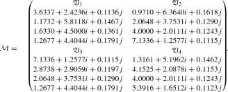
• Step 2: Aggregate these values into $r_k$ using CN-IMWA operator and get: $r_1=1.3365+ 6.6404 i +0.1127 j$, $r_2=1.9336 + 4.6104 i + 0.1122 j$, $r_3=2.2572 + 3.8979 i + 0.1137 j$, $r_4=2.7512 + 3.2622 i + 0.1114 j$.

• Step 3: By Eq. (12), the matrix ${\mathcal {P}}$ is obtained as:

  $$\begin{aligned} {\mathcal {P}}= \begin{pmatrix} 0.5000 &{} 0.3387 &{} 0.2571 &{} 0.1497 \\ 0.6613 &{} 0.5000 &{} 0.4174 &{} 0.3061 \\ 0.7429 &{} 0.5826 &{} 0.5000 &{} 0.3872 \\ 0.8503 &{} 0.6939 &{} 0.6128 &{} 0.5000 \\ \end{pmatrix}. \end{aligned}$$

  (35)

• Step 4: By Eq. (32), degrees of each alternative are obtained as $\theta _1 = 0.1871$; $\theta _2=0.2404$; $\theta _3=0.2677$; $\theta _4=0.3048$; and get ${\mathcal {K}}_4\succ {\mathcal {K}}_3\succ {\mathcal {K}}_2\succ {\mathcal {K}}_1$ which is logical.

On the other hand, if we appropriate the existing approaches [17, 18, 22, 27, 50] (steps are eliminated here) to aggregate the furnished data, then their analogous outcomes are placed in Table 14. From this table, it is comprehended that the best alternative inhabits the same, i.e., ${\mathcal {K}}_4$.

Table 14 Comparative analysis of Example 15

Table 15 Computed results of Example 16

Example 16

For an MADM problem with two alternatives ${\mathcal {K}}_1$ and ${\mathcal {K}}_2$ under four attributes ${\mathfrak {B}}_1$, ${\mathfrak {B}}_2$, ${\mathfrak {B}}_3$, and ${\mathfrak {B}}_4$ having weights $\omega =(0.4, 0.3, 0.1, 0.2)$. An expert gives their preference in terms of IMNs and represented their values as follows:

With the given weight vector and using the existing AOs [17, 18, 22, 27, 50], the aggregated values of ${\mathcal {K}}$s are summarized in Table 15.

It is contemplated that the aggregated values by the existing approaches [22, 50] are (9,1/9) or (1/9, 9) which is the greatest or least IMN, respectively.

On contrary to these, if we utilized the proposed MADM approach to this given information, then we construct the CN-IMNs of the given IMNs and are summarized in Eq. (36):

(36)

Based on this information, we aggregated the results using CN-IMWG operator and apply the proposed PDM on it to compute the final values of the alternatives. By Eq. (32), we get the optimal degree of ${\mathcal {K}}$s are $\theta _1= 0.75$ and $\theta _2= 0.25$. Since $\theta _1 > \theta _2$ and, thus, ${\mathcal {K}}_1$ is better than ${\mathcal {K}}_2$.

Example 17

Consider an MADM problem consists of ${\mathcal {K}}_1$ and ${\mathcal {K}}_2$ as alternatives and ${\mathfrak {B}}_1$, ${\mathfrak {B}}_2$ and ${\mathfrak {B}}_3$ as attributes with weight vector $\omega =(1/3,1/3,1/3)$. The information of the given alternatives is given as:

(37)

To address and rank the given alternative properly, we implemented the suggested approach on it and hence computed the CN-IMNs of the given numbers are summarized as:

Based on this information and by utilizing the proposed approach with CN-IMWA operator, we obtain the PDM as:

$$\begin{aligned} {\mathcal {P}}= \begin{pmatrix} 0.5000 &{} 0.4952 &{} 0.4456 \\ 0.5048 &{} 0.5000 &{} 0.4492 \\ 0.5544 &{} 0.5508 &{} 0.5000 \\ \end{pmatrix}. \end{aligned}$$

(38)

Thus, the final optimal values of the alternatives by Eq. (32) as $\theta _1=0.3235$, $\theta _2=0.3257$. and $\theta _3=0.3509$. From this analysis, we conclude that ${\mathcal {K}}_3$ is preferable over ${\mathcal {K}}_1$ and ${\mathcal {K}}_2$.

Advantages of the proposed framework

From the figured decisions reviewed in Tables 6, 7, 10, 12, 13,  14, and 15, it is perceived that the ranking index of the inherited process may somewhat deviate from the current designs. This is anticipated to specific deductions, which are illustrated here:

• (1) The existing strategies supporting the category of IMS to determine the DMPs have set a restraint on the MD and NMD only. However, the stated theory yields an alternative space to share with the problem with three degrees namely “contrary”, “identity”, and “discrepancy” of the CNs, such that their outcome is equal to one. The compatibility between the SPA and IMS proffers a proper mode to transform the given IMN into CN-IMN, which is described in Definition 8 and Definition 9. Hence, the given work is more prudish to solve modern decision-making problems, and there is a definite lessen the lack of information during the execution process.

• (2) The traditional operators [17, 18, 22, 27, 50] under the IMS environment are expressed outwardly examining the degree of hesitancy in the study. The consequences of such are explained in Examples 7, 8. To defeat these hindrances, some new weighted operators are introduced by holding all the degrees.

• (3) The ranking procedures in the conventional methods are prepared by $S({\mathcal {M}})=\vartheta /\varphi$ for IMN ${\mathcal {M}}=(\vartheta ,\varphi )$, which have sparse impediments as revealed in Examples 4, 5. Also, it is perceived that the score function is extremely sensitive to a non-membership degree of $\varphi$. To succeed it, in the stated algorithm, the PDM is adopted to rank the numbers, by consolidating the hesitancy degree, which has, fortunately, defeat the deficiencies of the existing ranking measures. Thus, the applicability scope of the advised process is more comprehensive than the present ones.

Conclusion

The chief augmentation of the work is compiled below.

• (1) A new concept of CN-IMNs for the IMSs is formed by combining the features of “identity”, “contrary”, and “discrepancy” degrees of the set into the one consolidated system. The explained CN-IMN ${\mathcal {C}}n=a+bi+cj$ affords an alternative way to trade with the uncertainties, such that $abc=1$. On the other hand, the existing IMS is features by the MD $\vartheta$ and NMD $\varphi$ only, such that $\vartheta \varphi \le 1$.

• (2) It has been noted that the existing functions namely score or accuracy under the IMS decline to match the objects. The faults of its are shown in detail (Examples 4, 5). To defeat the drawbacks of it, a more generalized PDM for the pairs of CN-IMNs is created to match the given objects. Also, the performance as well as interests of the stated PDM are confirmed by the examples as given in Example 15–17. Apart from it, the existing measures have counted only the MDs and NMDs of IMSs and remove the degree of hesitancy during the process. On the other hand, the proposed PDM estimates more objective information in terms of CN degrees, and consequently, the proposed approach can completely prevent any loss of information.

• (3) The MAGDM algorithm based on the recommended operators is explained, which is more generalized and flexible with the parameter q to the decision-maker. The significance of the different AOs on final ranking is shown in detail (Table 5). Associated with the several existing MAGDM algorithm (Tables 6, 7, 10, 12, 13,  14, and 15) under diverse fuzzy environment, the advantages are: (i) get the optimal alternatives by taking all the degrees such as “contrary”, “identity”, and “discrepancy” into the analysis; (ii) employ the novel PDM to order the given alternatives rather than existing score function which may give the effects sometimes irregular as demonstrated in the above Examples 3–8.

In the future, we expect to work in operating the proposed approaches in some other real-life scenarios such as “medical diagnosis”, “pattern recognition”, and “brain hemorrhage” [51, 52]. Also, there is a wide scope to enhance the theory to the different kinds of fuzzy sets such as neutrosophic set, m-polar set, Pythagorean set, etc., [53,54,55,56,57]. Moreover, we shall discuss the applications of these notions in the different fields, such as pattern recognition, artificial intelligence, social sciences, and many other fields.

References

Zadeh LA (1965) Fuzzy sets. Inf Control 8:338–353
Atanassov KT (1986) Intuitionistic fuzzy sets. Fuzzy Sets Syst 20(1):87–96
Atanassov K, Gargov G (1989) Interval-valued intuitionistic fuzzy sets. Fuzzy Sets Syst 31:343–349
Garg H, Kumar K (2019) Linguistic interval-valued Atanassov intuitionistic fuzzy sets and their applications to group decision-making problems. IEEE Trans Fuzzy Syst 27(12):2302–2311
Xu ZS (2007) Intuitionistic fuzzy aggregation operators. IEEE Trans Fuzzy Syst 15:1179–1187
Xu ZS, Yager RR (2006) Some geometric aggregation operators based on intuitionistic fuzzy sets. Int J Gen Syst 35:417–433
Chen SM, Cheng SH, Lan TC (2016) A novel similarity measure between intuitionistic fuzzy sets based on the centroid points of transformed fuzzy numbers with applications to pattern recognition. Inf Sci 343–344:15–40
Gou XJ, Xu ZS, Lei Q (2016) New operational laws and aggregation method of intuitionistic fuzzy information. J Intell Fuzzy Syst 30:129–141
Ejegwa PA, Onyeke IC, Adah V (2020) An algorithm for an improved intuitionistic fuzzy correlation measure with medical diagnostic application. Ann Optim Theory Pract. https://doi.org/10.22121/AOTP.2020.249456.1041
De SK (2020) Decision making under intuitionistic fuzzy metric distances. Ann Optim Theory Practi. https://doi.org/10.22121/AOTP.2020.250749.1043
Mahmood T, Ullah K, Jan N, Ahmad Z (2020) Policy decision making based on some averaging aggregation operators of t-spherical fuzzy sets: a multi-attribute decision making approach. Ann Optim Theory Pract. https://doi.org/10.22121/AOTP.2020.241244.1035
Garg H (2019) Intuitionistic fuzzy Hamacher aggregation operators with entropy weight and their applications to multi-criteria decision-making problems. Iran J Sci Technol Trans Electr Eng 43(3):597–613
Yang Z, Garg H, Li J, Srivastavad G, Cao Z (2020) Investigation of multiple heterogeneous relationships using a q-rung orthopair fuzzy multi-criteria decision algorithm. Neural Comput Appl. https://doi.org/10.1007/s00521-020-05003-5
Saaty TL (1986) Axiomatic foundation of the analytic hierarchy process. Manag Sci 32(7):841–845
Kaur G, Garg H (2018) Cubic intuitionistic fuzzy aggregation operators. Int J Uncertainty Quantif 8(5):405–427
Kaur G, Garg H (2019) Generalized cubic intuitionistic fuzzy aggregation operators using t-norm operations and their applications to group decision-making process. Arab J Sci Eng 44(3):2775–2794
Xia M, Xu Z, Liao H (2013) Preference relations based on intuitionistic multiplicative information. IEEE Trans Fuzzy Syst 21(1):113–132
Garg H (2018) Generalized interaction aggregation operators in intuitionistic fuzzy multiplicative preference environment and their application to multicriteria decision-making. App Intell 48(8):2120–2136
Yu S, Xu ZS (2014) Aggregation and decision making using intuitionistic multiplicative triangular fuzzy information. J Syst Sci Syst Eng 23:20–38
Jiang Y, Xu Z, Gao M (2015) Methods for ranking intuitionistic multiplicative numbers by distance measures in decision making. Comput Ind Eng 88:100–109
Garg H (2017) Distance and similarity measure for intuitionistic multiplicative preference relation and its application. Int J Uncertainty Quantif 7(2):117–133
Qian W, Niu L (2016) Intuitionistic multiplicative preference relation and its application in group decision making. J Intell Fuzzy Syst 30(5):2859–2870
Xia MM, Xu ZS (2013) Group decision making based on intuitionistic multiplicative aggregation operators. Appl Math Model 37:5120–5133
Yu DJ, Fang LC (2014) Intuitionistic multiplicative aggregation operators with their application in group decision making. J Intell Fuzzy Syst 27:131–142
Xia M (2015) Point operators for intuitionistic multiplicative information. J Intell Fuzzy Syst 28(2):615–620
Garg H (2018) Novel correlation coefficients under the intuitionistic multiplicative environment and their applications to decision-making process. J Ind Manag Optim 14(4):1501–1519
Garg H (2016) Generalized intuitionistic fuzzy multiplicative interactive geometric operators and their application to multiple criteria decision making. Int J Mach Learn Cybern 7(6):1075–1092
Jiang Y, Xu Z (2014) Aggregating information and ranking alternatives in decision making with intuitionistic multiplicative preference relations. Appl Soft Comput 22:162–177
Garg H (2017) A robust ranking method for intuitionistic multiplicative sets under crisp, interval environments and its applications. IEEE Trans Emerg Top Comput Intell 1(5):366–374
Jiang Y, Xu Z, Yu X (2013) Compatibility measures and consensus models for group decision making with intuitionistic multiplicative preference relations. Appl Soft Comput 13(4):2075–2086
Ren PJ, Xu ZS, Liao HC (2016) Intuitionistic multiplicative analytic hierarchy process in group decision making. Comput Ind Eng 101:513–524
Zhang Z, Pedrycz W (2018) Intuitionistic multiplicative group analytic hierarchy process and its use in multicriteria group decision-making. IEEE Trans Cybern 48(7):1950–1962
Mou Q, Xu ZS, Liao HC (2016) An intuitionistic fuzzy multiplicative best-worst method for multi-criteria group decision-making. Inf Sci 374:224–239
Garg H (2020) Exponential operational laws and new aggregation operators for intuitionistic multiplicative set in multiple-attribute group decision making process. Inf Sci 538:245–272
Zhao K (1989) Set pair and set pair analysis-a new concept and systematic analysis method. In: Proceedings of the national conference on system theory and regional planning, pp 87–91
Jiang YL, Xu CF, Yao Y, Zhao KQ (2004) Systems information in set pair analysis and its applications. In: Proceedings of 2004 international conference on machine learning and cybernetics, vol. 3, pp 1717 – 1722
Liu C, Zhang L, Yang A (2013) The fundamental operation on connection number and its applications. J Theor Appl Inf Technol 49(2):618–623
Garg H, Kumar K (2019) An advanced study on operations of connection number based on set pair analysis. Natl Acad Sci Lett 42(4):351–354
Yang J, Zhou J, Liu L, Li Y, Wu Z (2008) Similarity measures between connection numbers of set pair analysis. Springer, Berlin, pp 63–68. https://doi.org/10.1007/978-3-540-87732-5
Yang FG, Liang Y, Singh VP, Wang WS, Zhou XQ, Liu XN, Cao SY, Huang E, Wu YH (2014) Debris flow hazard assessment using set pair analysis models: take Beichuan county as an example. J Mt Sci 11(4):1015–1022
Hu J, Yang L (2011) Dynamic stochastic multi-criteria decision making method based on cumulative prospect theory and set pair analysis. Syst Eng Procedia 1:432–439
Xie Z, Zhang F, Cheng J, Li L (2013) Fuzzy multi-attribute decision making methods based on improved set pair analysis. In: Sixth international symposium on computational intelligence and design, vol 2, pp 386 – 389
Kumar K, Garg H (2018) TOPSIS method based on the connection number of set pair analysis under interval-valued intuitionistic fuzzy set environment. Comput Appl Math 37(2):1319–1329
Kumar K, Garg H (2018) Connection number of set pair analysis based TOPSIS method on intuitionistic fuzzy sets and their application to decision making. Appl Intell 48(8):2112–2119
Garg H, Kumar K (2020) A novel exponential distance and its based TOPSIS method for interval-valued intuitionistic fuzzy sets using connection number of SPA theory. Artif Intell Rev 53(1):595–624
Riaz M, Tehrim ST (2020) A robust extension of VIKOR method for bipolar fuzzy sets using connection numbers of SPA theory based metric spaces. Artif Intell Rev. https://doi.org/10.1007/s10462-020-09859-w
Garg H, Kumar K (2020) A novel possibility measure to interval-valued intuitionistic fuzzy set using connection number of set pair analysis and their applications. Neural Comput Appl 32(8):3337–3348
Cao YX, Zhou H, Wang JQ (2018) An approach to interval-valued intuitionistic stochastic multi-criteria decision-making using set pair analysis. Int J Mach Learn Cybernet 9(4):629–640
Shui XZ, Li DQ (2003) A possibility based method for priorities of interval judgment matrix. Chin J Manag Sci 11(1):63–65
Xu CY, Ma ZM (2019) Symmetric intuitionistic multiplicative aggregation operator for group decision making in intuitionistic multiplicative environments. J Intell Fuzzy Syst 36(6):5909–5918
Garg H (2020) Linguistic interval-valued Pythagorean fuzzy sets and their application to multiple attribute group decision-making process. Cogn Comput 12(6):1313–1337. https://doi.org/10.1007/s12559-020-09750-4
Garg H (2021) A new possibility degree measure for interval-valued q-rung orthopair fuzzy sets in decision-making. Int J Intell Syst 36(1):526–557. https://doi.org/10.1002/int.22308
Fahmi A, Amin F, Shah SBH (2020) Geometric operators based on linguistic interval-valued intuitionistic neutrosophic fuzzy number and their application in decision making. Ann Optim Theory Pract 3(1):47–71
Hashmi MR, Riaz M, Smarandache F (2020) m-polar neutrosophic topology with applications to multi-criteria decision-making in medical diagnosis and clustering analysis. Int J Fuzzy Syst 22(1):273–292
Riaz M, Davvaz B, Fakhar A, Firdous A (2020) Hesitant fuzzy soft topology and its applications to multi-attribute group decision-making. Soft Comput 24:16269–16289
Naeem K, Riaz M, Peng X, Afzal D (2019) Pythagorean fuzzy soft MCGDM methods based on TOPSIS, VIKOR and aggregation operators. J Intell Fuzzy Syst 37(5):6937–6957
Yang Z, Li X, Garg H, Qi M (2020) Decision support algorithm for selecting an antivirus mask over COVID-19 pandemic under spherical normal fuzzy environment. Int J Environ Res Public Health 17(10):3407. https://doi.org/10.3390/ijerph17103407
Author information
Authors and Affiliations
Corresponding author
Ethics declarations
Conflict of interest
The authors declare that they have no conflict of interest.
Additional information
Publisher's Note
Springer Nature remains neutral with regard to jurisdictional claims in published maps and institutional affiliations.
Rights and permissions
Open Access This article is licensed under a Creative Commons Attribution 4.0 International License, which permits use, sharing, adaptation, distribution and reproduction in any medium or format, as long as you give appropriate credit to the original author(s) and the source, provide a link to the Creative Commons licence, and indicate if changes were made. The images or other third party material in this article are included in the article’s Creative Commons licence, unless indicated otherwise in a credit line to the material. If material is not included in the article’s Creative Commons licence and your intended use is not permitted by statutory regulation or exceeds the permitted use, you will need to obtain permission directly from the copyright holder. To view a copy of this licence, visit http://creativecommons.org/licenses/by/4.0/.
About this article
Cite this article
Garg, H. Multi-attribute group decision-making process based on possibility degree and operators for intuitionistic multiplicative set. Complex Intell. Syst. 7, 1099–1121 (2021). https://doi.org/10.1007/s40747-020-00256-y
Received:
Accepted:
Published:
Issue Date:
DOI: https://doi.org/10.1007/s40747-020-00256-y