Synchronization of coupled benchmark oscillators: analysis and experiments

Abstract

Synchronization is a significant phenomenon in understanding the collective dynamics of coupled oscillators. It is important to know about the behavior and derive sufficient conditions that yield synchronization in coupled benchmark oscillators. The paper aims at achieving synchronization in two types of second-order coupled oscillators, namely the Van der Pol and the Fitzhugh Nagumo oscillators. The oscillators are coupled diffusively with uniform and non-uniform couplings. Initially, the network topology is taken as all-to-all connected, and its synchronization analysis is carried out using the quadratic Lyapunov approach. The algebraic graph theory is used to formulate a quadratic Lyapunov function to attain synchronization of the coupled oscillatory network with the arbitrarily connected network topologies of these oscillators. The couplings used are for both the states as well as for a single state. In each of the above cases, the synchronization is achieved by obtaining sufficient coupling gain. The synchronization has also been demonstrated experimentally for all-to-all and star networked oscillators. The analytical and experimental results have been compared for sufficient coupling gains. Also, the findings are supported by numerical simulation.

Appendices

Appendix A: Proof Theorem 4.2

We illustrate the proof in the case of N=4 oscillators as shown in Fig. 1.

The dynamical equations of four all-to-all coupled FHN oscillators can be obtained from (14) and (15) for N $=$ 4 oscillators. For simplicity,we use notations $K_{1},K_{2},K_{3},K_{4},K_{5 }, K_{6}$ in place of $K_{pi}=K_{ip}$ $\forall$ i,p = (1,..,4), $i\ne p$. We define following positive definite function presented below and find their derivatives along the corresponding difference dynamics which can be obtained from (14) and (15) for N $=$ 4 oscillators. Let,

$$\begin{aligned}&S_1= \frac{1}{2}[(v_1-v_2)^2+\frac{c}{db}(w_1-w_2)^2]. \end{aligned}$$

(34)

Similarly, $S_{2},S_{3}, S_{4},S_{5}$ and $S_{6}$ can be defined for each connection. Now,

$$\begin{aligned}&\dot{S}_1=(v_1-v_2)(\dot{v}_1-\dot{v}_2)+(w_1-w_2)(\dot{w}_1-\dot{w}_2)\frac{c}{db},\\&\quad \Rightarrow \dot{S}_1= (c-2K_1)(v_1-v_2)^2\\&\qquad -\frac{c}{3}(v_1-v_2)^2\left( \frac{v_1^2}{2}+\frac{v_2^2}{2}+\frac{(v_1+v_2)^2}{2}\right) \\&\qquad -K_2(v_3-v_2)(v_1-v_2)+K_4(v_4-v_1)(v_1-v_2)\\ {}&\quad \quad +K_5(v_3-v_1)(v_1-v_2)-K_6(v_4-v_2)(v_1-v_2)\\ {}&\quad -\frac{c}{b}(w_1-w_2)^2. \end{aligned}$$

Let S be a positive definite Lyapunov function given as

$$\begin{aligned}&S=S_1+S_2+S_3+S_4+S_5+S_6,\nonumber \\&\Rightarrow \dot{S}=\dot{S_1}+\dot{S_2}+\dot{S_3}+\dot{S_4}+\dot{S_5}+\dot{S_6}. \end{aligned}$$

(35)

On simplification and neglecting negative square terms, we get

$$\begin{aligned}&\dot{S}\le [(c-4K_1)(v_1-v_2)^2+(c-4K_2)(v_2-v_3)^2\\ {}&\quad \quad +(c-4K_3)(v_3-v_4)^2+(c-4K_4)(v_4-v_1)^2\\ {}&\quad \quad +(c-4K_5)(v_1-v_3)^2+(c-4K_6)(v_4-v_2)^2\\ {}&\quad \quad -\frac{c}{b}[(w_1-w_2)^2+(w_2-w_3)^2+(w_3-w_4)^2\\ {}&\qquad +(w_4-w_1)^2+(w_1-w_3)^2+(w_4-w_2)^2] \end{aligned}$$

Therefore, $\dot{S}$ is negative definite if each of the coupling gain $K_{i}\ge c/4, \forall i= (1,\ldots ,6)$. Hence, the four non-uniformly linearly coupled FHN oscillators synchronize asymptotically as $t\rightarrow \infty$. Analogous results for any number of coupled oscillators can be derived similarly. $\blacksquare$

Appendix B: Proof of theorem 5.2 exponential synchronization of coupled FHN oscillators

Let V represent a vector of all states $v_{i}$. Similarly, let W represents a vector of all states $w_{i}$, $\forall i=(1,\ldots ,N)$. Also, let $\tilde{V}=V-\bar{V}\Rightarrow \dot{\tilde{V}}=\dot{V}-\dot{\bar{V}}$ and $\tilde{W}=W-\bar{W}\Rightarrow \dot{\tilde{W}}=\dot{W}-\dot{\bar{W}}$. Let $K_{p}$ be the sufficient coupling required in each connection for synchronization. Consider a Lyapunov function,

$$\begin{aligned}&S=\frac{1}{2}\tilde{V}^T\tilde{V}+\frac{c}{2db}\tilde{W}^T\tilde{W},\\&\dot{S}=\tilde{V}^T\dot{\tilde{V}}+\frac{c}{db}\tilde{W}^T\dot{\tilde{W}}.\nonumber \end{aligned}$$

(36)

It follows [21], $\tilde{V}^{T}L\tilde{V}$ $\ge \lambda _{2}(L)\tilde{V}^T\tilde{V}$ $\forall$ $\tilde{V} \perp 1_{N}$ and $\tilde{W}^{T}L\tilde{W}$ $\ge \lambda _{2}(L)\tilde{W}^T\tilde{W}$ $\forall$ $\tilde{W} \perp 1_{N}$.

$$\begin{aligned} \Rightarrow \dot{S}&=c(V-\bar{V})^{T}[(V-\bar{V})-(W-\bar{W})-\frac{1}{3}(V^{o3}-\bar{V}^{o3})]\nonumber \\ {}&\quad -\tilde{V}^TK_{p}L\tilde{V} +\frac{c}{db}(W-\bar{W})[db(V-\bar{V})-d(W-\bar{W})]\nonumber \\ {}&\quad -\tilde{W}^TK_{p}L\tilde{W}\times \frac{c}{db},\nonumber \\&\Rightarrow \dot{S}\le c(\tilde{V}^{T}\tilde{V})-\tilde{V}^TK_{p}L\tilde{V}-\frac{c}{b} (\tilde{W}^{T}\tilde{W})\nonumber \\ {}&\quad -\tilde{W}^TK_{p}L\tilde{W}\times \frac{c}{db}+c(\tilde{W}^{T}\tilde{W})-c(\tilde{W}^{T}\tilde{W}),\nonumber \\&\Rightarrow \dot{S}\le [c-\lambda _{2}(L)K_{p}][2S]. \end{aligned}$$

(37)

Let,

$$\begin{aligned}&[c-\lambda _{2}(L)K_{p}]=-\beta ,\\&\Rightarrow \dot{S}\le -\beta 2S,\\&\Rightarrow \dot{S}\le ||S_{o}||e^{-2\beta t}. \end{aligned}$$

Thus, for exponential synchronization of coupled FHN oscillators in arbitrary connected network topology, each coupling gain,

$$\begin{aligned} K_{p}>c/{\lambda _{2}(L)} \end{aligned}$$

(38)

Appendix C: Comparison with [13]

The FHN dynamics which we consider is the special case of the dynamics considered in [13]. Furthermore, the sufficiency condition of synchronization on coupling gain, which we obtain using the quadratic Lyapunov analysis i.e. $K\ge c/N$ as found in Theorem 5.2, is the same as the sufficiency condition of synchronization in similar coupled oscillator dynamics using the Partial Contraction analysis in example 4.4 in [13]. Its statement is illustrated below. The authors have considered a diffusively coupled network with N-identical FHN oscillators, as presented below:

$$\begin{aligned}&\dot{v_{i}}=c\left[ v_{i}-w_{i}-\frac{1}{3}v_{i}^3\right] +I+\sum _{j\in {N_{i}}}k_{ij}(v_{j}-v_{i}), \end{aligned}$$

(39)

$$\begin{aligned}&\dot{w_{i}}=-\frac{1}{c}[v_{i}-a+bw_{i}]\quad \quad \quad \quad i=(1,\ldots ,n). \end{aligned}$$

(40)

Here, a, b, c are the parameters. As per Theorem 6 on page 13, the whole network synchronizes exponentially if,

$$\begin{aligned} \lambda _{2}\left( \sum _{(ij)\in {N}}^bT_{k_{ij}}^n\right) >c, \end{aligned}$$

Where,

$$\begin{aligned} T_{k_{ij}}^n = \begin{bmatrix} \ddots &{}\vdots &{} &{}\vdots &{} \\ \cdots &{} \mathbf {K} &{} \cdots &{} -\mathbf {K} &{} \cdots \\ &{}\vdots &{} \ddots &{} \vdots &{} \\ \cdots &{} -\mathbf {K} &{}\cdots &{}\mathbf {K} &{} \cdots \\ &{}\vdots &{} &{} \vdots &{} \ddots \\ \end{bmatrix}_{n \times n} \end{aligned}$$

All the elements in $T_{k_ij}^n$, except those displayed above at the four intersections of $i^{th}$ and $j^{th}$ columns are zero. One has $T_{k_ij}^n$=0 if K=0. Also, $N=\cup _{i=1}^nN_{i}$ denote a set of active links in the network. The authors have proved using Partial Contraction analysis that the coupling gain sufficient to give synchronization among the linearly coupled FHN models should be such that $k_{ij}\ge c/N$.

Appendix D: Comparison with [21]

In [21], the authors studied the reaction-diffusion PDE system, which is presented as,

$$\begin{aligned}&\frac{\partial x}{\partial t}=f(x)+D\triangledown ^2x, \end{aligned}$$

(41)

subjected to the Neumann boundary condition and given a condition on the uniform behavior of its solution. The main result (Theorem 1) requires the following Lyapunov inequality to be satisfied by the matrix. $(J(x)-\lambda _{2}D)$.

$$\begin{aligned}&P(J(x)-\lambda _{2}D)+(J(x)-\lambda _{2}D)^TP\le -\epsilon I, \end{aligned}$$

(42)

where $\lambda _{2}$ is a measure of the well connectedness of the spatial domain. They illustrated the same by taking an example of FHN oscillators with augmented diffusion terms, which is stated below:

$$\begin{aligned}&\frac{\partial x_{1}}{\partial t}=c\left( x_{1}-\frac{1}{3}x^3_{1}+x_{2}\right) +d_1\triangledown ^2x_{1},\\&\frac{\partial x_{2}}{\partial t}=\frac{1}{c}(-x_{1}-bx_{2}+a)+d_2\triangledown ^2x_{2}, \end{aligned}$$

The Jacobian matrix is stated as,

$$\begin{aligned} J(x)=\begin{bmatrix}c(1-x^2_1) &{} b \\ -1/c &{} -b/c \end{bmatrix} \end{aligned}$$

For,

$$\begin{aligned} P=\begin{bmatrix}1/c&{} 0\\ 0 &{} c \end{bmatrix} \end{aligned}$$

The inequality (42) holds and yields that synchronization is guaranteed if $\lambda _{2}> c/d_{1}$. Here, the term $d_{1}$ represents coupling gain. This is the same as our synchronization condition using the quadratic Lyapunov function approach, which requires minimum coupling gain $K_{ij}\ge c/N$. This corroboration gives strength to our results.

Appendix E: Laplacian matrices of ring, chain, star, random topology networks

• 1. Ring of four oscillators:

  

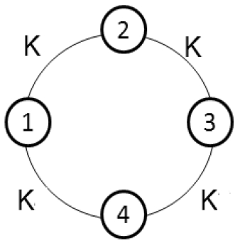  $$\begin{aligned} D=\begin{bmatrix}2 &{} 0 &{} 0 &{} 0 \\ 0 &{} 2 &{} 0 &{} 0 \\ 0 &{} 0 &{} 2 &{} 0 \\ 0 &{} 0 &{} 0 &{} 2 \end{bmatrix} , A=\begin{bmatrix}0 &{} 1 &{} 0 &{} 1 \\ 1 &{} 0 &{} 1 &{} 0 \\ 0 &{} 1 &{} 0 &{} 1 \\ 1 &{} 0 &{} 1 &{} 0 \end{bmatrix}, \end{aligned}$$

  and the graph laplacian matrix $L = D-A$,

  $$\begin{aligned} L=\begin{bmatrix}2 &{} -1 &{} 0 &{} -1 \\ -1 &{} 2 &{} -1 &{} -1 \\ 0 &{} -1 &{} 2 &{} -1 \\ -1 &{} 0 &{} -1 &{} 2 \end{bmatrix}. \end{aligned}$$

  Thus, the sufficiency condition for exponential synchronization is $K_{p}>\mu /2$.

• 2. Chain network of four oscillators:

  

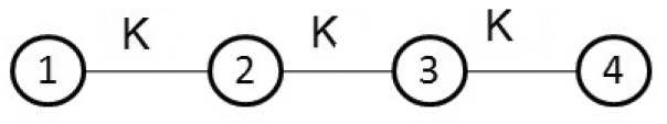  $$\begin{aligned} D=\begin{bmatrix}1 &{} 0 &{} 0 &{} 0 \\ 0 &{} 2 &{} 0 &{} 0 \\ 0 &{} 0 &{} 2 &{} 0 \\ 0 &{} 0 &{} 0 &{} 1 \end{bmatrix}, A=\begin{bmatrix}0 &{} 1 &{} 0 &{} 0 \\ 1 &{} 0 &{} 1 &{} 0 \\ 0 &{} 1 &{} 0 &{} 1 \\ 0 &{} 0 &{} 1 &{} 0 \end{bmatrix}, \end{aligned}$$

  and the graph Laplacian matrix $L = D-A$,

  $$\begin{aligned} L=\begin{bmatrix}1 &{} -1 &{} 0 &{} 0 \\ -1 &{} 2 &{} -1 &{} 0 \\ 0 &{} -1 &{} 2 &{} -1 \\ 0 &{} 0 &{} -1 &{} 1 \end{bmatrix} \end{aligned}$$

  Thus, the sufficiency condition for exponential synchronization is $K_{p}>\mu /0.58$.

• 3. Star network of five oscillators:

  

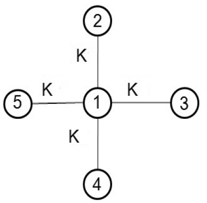  $$\begin{aligned} D=\begin{bmatrix}4 &{} 0 &{} 0 &{} 0 &{} 0 \\ 0 &{} 1 &{} 0 &{} 0 &{} 0 \\ 0 &{} 0 &{} 1 &{} 0 &{} 0 \\ 0 &{} 0 &{} 0 &{} 1 &{} 0\\ 0 &{} 0 &{} 0 &{} 0 &{} 1 \end{bmatrix}, A=\begin{bmatrix}0 &{} 1 &{} 1 &{} 1 &{} 1 \\ 1 &{} 0 &{} 0 &{} 0 &{} 0 \\ 1 &{} 0 &{} 0 &{} 0 &{} 0 \\ 1 &{} 0 &{} 0 &{} 0 &{} 0\\ 1 &{} 0 &{} 0 &{} 0 &{} 0 \end{bmatrix}, \end{aligned}$$

  and the graph Laplacian matrix $L = D-A$,

  $$\begin{aligned} L=\begin{bmatrix}4 &{} -1 &{} -1 &{} -1 &{} -1 \\ -1 &{} 1 &{} 0 &{} 0 &{} 0 \\ -1 &{} 0 &{} 1 &{} 0 &{} 0 \\ -1&{} 0 &{} 0 &{} 1 &{} 0\\ -1 &{} 0 &{} 0 &{} 0 &{} 1 \end{bmatrix} \end{aligned}$$

  Thus, the sufficiency condition for exponential synchronization is $K_{p}>\mu /1$.

• 4. Arbitrary connected network of six oscillators:

  

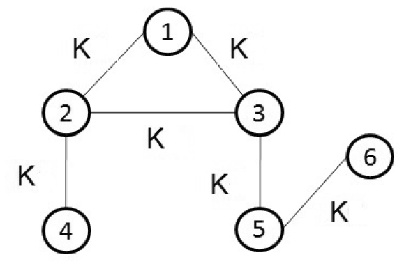  $$\begin{aligned}&D=\begin{bmatrix}2 &{} 0 &{} 0 &{} 0 &{} 0 &{} 0 \\ 0&{} 3 &{} 0 &{} 0 &{} 0 &{} 0 \\ 0&{} 0&{} 3 &{} 0 &{} 0 &{} 0\\ 0&{} 0 &{} 0 &{} 1 &{} 0 &{} 0&{}\\ 0&{} 0 &{} 0 &{} 0 &{} 2 &{} 0\\ 0&{} 0 &{} 0 &{} 0 &{} 0 &{} 1\end{bmatrix}, \\&A=\begin{bmatrix}0 &{} 1 &{} 1 &{} 0 &{} 0 &{} 0 \\ 1&{} 0&{} 1 &{} 1 &{} 0 &{} 0 \\ 1&{} 1&{} 0 &{} 0 &{} 1 &{} 0\\ 0&{} 1 &{} 0 &{} 0 &{} 0 &{} 0&{}\\ 0&{} 0 &{} 1 &{} 0 &{} 0 &{} 1\\ 0&{} 0 &{} 0 &{} 0 &{} 1 &{} 0\end{bmatrix} \end{aligned}$$

  and the graph laplacian matrix $L = D-A$,

  $$\begin{aligned} L=\begin{bmatrix}2&{} -1&{} -1 &{} 0 &{} 0 &{} 0 \\ -1 &{} 3 &{}-1 &{}-1 &{} 0 &{}0 \\ -1 &{} -1 &{} 3 &{} 0 &{} -1 &{} 0 \\ 0 &{}-1 &{} 0 &{} 1 &{} 0 &{} 0 \\ 0 &{} 0 &{}-1 &{} 0 &{} 2 &{}-1\\ 0 &{} 0 &{} 0 &{} 0 &{}-1 &{} 1\end{bmatrix}, \end{aligned}$$

  Thus, the sufficiency condition for exponential synchronization is $K_{p}>\mu /0.41$.

Appendix F: Simulations

The detailed simulations for various types of topologies comprising of the VDP as well as the FHN type of oscillators are illustrated below in Figs. 16, 17, 18, 19 and Figs. 20, 21, 22 and 23. It is interesting to note that in initially, each case unsynchronized oscillations of the uncoupled oscillators are observed. However, after the introduction of coupling gains at t=100 secs, synchronization of the coupled oscillators is achieved. The analytical findings, therefore, seek support from the simulation results.

Fig. 16

Synchronization of four (N=4) uniformly linearly coupled VDP oscillators which are connected in ring topology, for $\mu =1$ and each of the coupling gains $K>\mu /2$, turned on at t=100 secs

Fig. 17

Synchronization of four ($N=4$) uniformly linearly coupled VDP oscillators which are connected in a chain topology, for $\mu =1$ and each of the coupling gains $K>\mu /0.58$,turned on at $t=100$ s

Fig. 18

Synchronization of five ($N=5$) uniformly linearly coupled VDP oscillators which are connected in star topology, for $\mu =1$ and each of the coupling gains $K>\mu /1$, turned on at $t=100$ s

Fig. 19

Synchronization of six ($N=6$) uniformly linearly coupled VDP oscillators which are connected in arbitrary connected topology, for $\mu =1$ and each of the coupling gains $K>\mu /0.41$, turned on at $t=100$ s

Fig. 20

Synchronization of four ($N=4$) uniformly linearly coupled FHN oscillators which are connected in ring topology, for$c=1$ and each of the coupling gains $K>c/2$, turned on at $t=100$ s

Fig. 21

Synchronization of four ($N=4$) uniformly linearly coupled FHN oscillators which are connected in a chain topology, for $c=1$ and each of the coupling gains $K>c/0.58$, turned on at $t=100$ s

Fig. 22

Synchronization of five ($N=5$) uniformly linearly coupled FHN oscillators which are connected in star topology, for $c=1$ and each of the coupling gains $K>c/1$, turned on at $t=100$ s

Fig. 23

Synchronization of six ($N=6$) uniformly linearly coupled FHN oscillators which are connected in arbitrary connected topology, for $c=1$ and each of the coupling gains $K>c/0.41$, turned on at $t=100$ s

Appendix G: Experimental results

Electronic circuit, experimental set-up, and experimental observation of unsynchronized and synchronized oscillations of the VDP oscillators are shown in Figs. 24, 25, 26, 27, 28 and 29. Analogous figures for FHN oscillators are reported in Figs. 30, 31, 32, 34 and 35.

Fig. 24

Circuit diagram of four star coupled VDP oscillators

1.1 Four star coupled VDP oscillators

In terms of circuit parameters, the dynamics of four star coupled VDP oscillators (Fig. 24) are,

$$\begin{aligned}&\dot{x}_{1}=\frac{R_{4}}{R_{1}R_{3}C_{1}}x_{2},\\&\dot{x}_{2}=\frac{-x_{2}}{R_{2}C_{2}}-\frac{R_{4}}{ R_{3}R_{5}C_{2}}x_{2}(x_{1}^2-1)+\frac{1}{RC_{2}}(x_{4}-x_{2}),\\&\qquad +\frac{1}{RC_{2}}(x_{6}-x_{2})+\frac{1}{RC_{2}}(x_{8}-x_{2}),\\&\dot{x}_{3}=\frac{R_{4}}{R_{1}R_{3}C_{1}}x_{4},\\&\dot{x}_{4}=\frac{-x_{4}}{R_{2}C_{2}}-\frac{R_{4}}{ R_{3}R_{5}C_{2}}x_{4}(x_{3}^2-1)+\frac{1}{RC_{2}}(x_{2}-x_{4}),\\&\dot{x}_{5}=\frac{R_{4}}{R_{1}R_{3}C_{1}}x_{6},\\&\dot{x}_{6}=\frac{-x_{6}}{R_{2}C_{2}}-\frac{R_{4}}{ R_{3}R_{5}C_{2}}x_{6}(x_{5}^2-1)+\frac{1}{RC_{2}}(x_{2}-x_{6}),\\&\dot{x}_{7}=\frac{R_{4}}{R_{1}R_{3}C_{1}}x_{8},\\&\dot{x}_{8}=\frac{-x_{8}}{R_{2}C_{2}}-\frac{R_{4}}{ R_{3}R_{5}C_{2}}x_{8}(x_{5}^2-1)+\frac{1}{RC_{2}}(x_{2}-x_{8}). \end{aligned}$$

For $R_{5}=2.5 K\Omega$, $\mu =4$. As per analytical outcomes, the sufficient coupling gain for synchronization should be such that $K>\mu /\lambda _{2}(L)$, where $\mu =\frac{R_{4}}{R_{3}R_{5}C_{2}}$. In the present case, it should be $K>4$ per $\Omega -F$ while during experimentations, it was observed that $K=\frac{1}{RC_{2}}$. It was found through experimentations that synchronization occurred among coupled oscillators when the feedback resistance $R\le 2200$ $\Omega$. The corresponding coupling gain in terms of the circuit parameters is stated as $K=\frac{1}{2200 \times 0.1 mF}=4.5$ per $\Omega -F$. Thus, for the present case, it can again be experimentally said that more coupling gain is required than the analytical value to synchronize four star coupled VDP oscillators.

Fig. 25

Experimental set-up of four star coupled VDP oscillators

Fig. 26

Unsynchronized VDP oscillations

Fig. 27

Synchronization error

Fig. 28

Synchronized VDP oscillations

Fig. 29

Synchronization error

Fig. 30

Circuit diagram four star coupled FHN oscillators

1.2 Three all-to-all coupled FHN oscillators

The dynamics of three all-to-all coupled FHN oscillators in terms of their circuit parameters for Fig. 10 are stated as,

$$\begin{aligned}&\frac{\epsilon dV_{1}}{d\tau }=I_{o}-I_{1}-G(V_{1})+\frac{100}{R}(V_{2}-V_{1})+\frac{100}{R}(V_{3}-V_{1}),\\&\frac{dI_{1}}{d\tau }=\beta V_{1}-I_{1}-V_{o},\\&\frac{\epsilon dV_{2}}{d\tau }=I_{o}-I_{2}-G(V_{2})+\frac{100}{R}(V_{1}-V_{2})+\frac{100}{R}(V_{3}-V_{2}),\\&\frac{dI_{2}}{d\tau }=\beta V_{2}-I_{1}-V_{o}\\&\frac{\epsilon dV_{3}}{d\tau }=I_{o}-I_{3}-G(V_{3})+\frac{100}{R}(V_{1}-V_{3})+\frac{100}{R}(V_{2}-V_{3}),\\&\frac{dI_{3}}{d\tau }=\beta V_{3}-I_{3}-V_{o}. \end{aligned}$$

As per analytical outcome, the sufficient coupling gain for synchronization should be such that $K>c/N$. In the present case it should be $K=(1/3\epsilon )=((R1+R4)C_{2})/R_{1}C_{1}=258/3=86$. It was found through experimentations that when feedback resistance $R\le 235\Omega$, synchronization occurred among networked oscillators. In terms of circuit parameters, the corresponding coupling gain is stated as $K=\frac{100}{R\epsilon }=109.78$. Thus, for the present case, experimentally, the coupling gain required to synchronize three all-to-all coupled FHN oscillators is more than the analytical value.

1.3 Four star coupled FHN oscillators

In terms of the circuit parameters, the dynamics of four star coupled FHN oscillators (Fig. 30) are,

$$\begin{aligned}&\frac{\epsilon dV_{1}}{d\tau }=I_{o}-I_{1}-G(V_{1})+\frac{100}{R}(V_{2}-V_{1})+\frac{100}{R}(V_{3}-V_{1})\\ {}&\quad +\,\frac{100}{R}(V_{4}-V_{1}),\\&\frac{dI_{1}}{d\tau }=\beta V_{1}-I_{1}-V_{o},\\&\frac{\epsilon dV_{2}}{d\tau }=I_{o}-I_{2}-G(V_{2})+\frac{100}{R}(V_{1}-V_{2}),\\&\frac{dI_{2}}{d\tau }=\beta V_{2}-I_{1}-V_{o},\\&\frac{\epsilon dV_{3}}{d\tau }=I_{o}-I_{3}-G(V_{3})+\frac{100}{R}(V_{1}-V_{3}),\\&\frac{dI_{3}}{d\tau }=\beta V_{3}-I_{3}-V_{o},\\&\frac{\epsilon dV_{4}}{d\tau }=I_{o}-I_{4}-G(V_{4})+\frac{100}{R}(V_{1}-V_{4}),\\&\frac{dI_{4}}{d\tau }=\beta V_{4}-I_{4}-V_{o}. \end{aligned}$$

As per the analytical outcome, the sufficient coupling gain for synchronization should be such that $K>c/\lambda _{2}(L)$. In the present case, $(1/\epsilon )=((R1+R4)C_{2})/R_{1}C_{1}=258/1=258$. However, experimentally, it was found that synchronization in coupled oscillators is achieved if the series resistance in the feedback path is less than or equal to $70\Omega$. According to the experimentation, $K=\frac{100}{R\epsilon }=\frac{258\times 100}{70} =368$. Again, it is observed that the experimental threshold for coupling is higher than the analytical value of the threshold.

Fig. 31

Experimental set-up of four star coupled FHN oscillators

Fig. 32

Unsynchronized FHN oscillations

Fig. 33

Synchronization error

Fig. 34

Synchronized FHN oscillations

Fig. 35

Synchronization error

Appendix H: Synchronization of arbitrary connected coupled FHN oscillators using a single state coupling

Consider the following dynamics:

$$\begin{aligned}&\dot{V}= c\left[ V-W-\frac{1}{3}v^{o3}\right] -K_{p}LV,\\&\dot{W}= d[a\times 1_{N} + bV -W], \end{aligned}$$

Let,

$$\begin{aligned}&S=\frac{1}{2}\tilde{V}^T\tilde{V}+\frac{c}{2db}\tilde{W}^T\tilde{W} \Rightarrow \dot{S}=\tilde{V}^T\dot{\tilde{V}} +\frac{c}{db}\tilde{W}^T\dot{\tilde{W}},\\&\dot{S}=c(V-\bar{V})^{T}\left[ (V-\bar{V})-(W-\bar{W})-\frac{1}{3}(V^{o3}-\bar{V}^{o3})\right] ,\\ {}&\quad -\tilde{V}^TK_{p}L\tilde{V} +\frac{c}{db}(W-\bar{W})^{T}[db(V-\bar{V})-d(W-\bar{W})],\\&\dot{S}\le [c-\lambda _{2}(L)]\tilde{V}^{T}\tilde{V}-\frac{c}{b}\tilde{W}^{T}\tilde{W}. \end{aligned}$$

Thus, $\dot{S} <0$ if $K_{p}>\frac{c}{\lambda _{2}(L)}$. $\blacksquare$

References

Strogatz, SH (2018) Nonlinear dynamics and chaos: with applications to physics, biology, chemistry, and engineering. CRC Press, Taylor and Francis
Pikovsky A, Kurths J, Rosenblum M, Kurths J (2003) Synchronization: a universal concept in nonlinear sciences, vol 12. Cambridge University Press, Cambridge
Za’balawi I, Kiong LC, Kiong WE (2010) Synergetic brain model for human-like motion patterns recognition. In: 2010 International conference on computer applications and industrial electronics. IEEE, pp 374–378
Ahmed SH, Javed S, Abbas SK, Hussain S (2016) Modified van der pol (Vdp) oscillator based cardiac pacemakers. In: 2016 19th international conference on computer and information technology (ICCIT). IEEE, pp 176–183
Ahmad U, Ijaz Q, ul Husnain A (2015) Stability analysis of coupled van der pol’s oscillator. In: 2015 13th international conference on frontiers of information technology (FIT). IEEE, pp 24–29
Barrón MA, Sen M (2009) Synchronization of four coupled van der Pol oscillators. Nonlinear Dyn 56(4):357–367
Barron Miguel A, Medina Dulce Y, Isaias H (2014) Collective behavior of a ring of Van der Pol oscillators under Gaussian and random coupling schemes. Open Journal of Applied Sciences, Scientific Research
Gan K-J, Jiang Z-J, Chan D-Y, Tsai C-S, Huang J-S, Kao Z-K, Yeh W-K (2013) Design and application of Van Der Pol oscillator using NDR circuit. In: 2013 International symposium on next-generation electronics. IEEE, pp 329–332
Vaidyanathan S (2015) Adaptive synchronization of the identical FitzHugh–Nagumo chaotic neuron models. Int J PharmTech Res 8(6):167–177
Corinto, F, Lanza V, Ascoli A, Gilli M (2011) Synchronization in networks of FitzHugh–Nagumo neurons with memristor synapses. In: 2011 20th European conference on circuit theory and design (ECCTD). IEEE, pp 608–611
Zhang, Q, Luo J, Liu J (2014) Robust consensus of FitzHugh–Nagumo networks with disturbances via sliding mode control. In: 2014 10th international conference on natural computation (ICNC). IEEE, pp 134–138
Bharath R, Slotine J-J (2013) Nonlinear observer design and synchronization analysis for classical models of neural oscillators. arXiv:1310.0479
Wang W, Slotine J-JE (2005) On partial contraction analysis for coupled nonlinear oscillators. Biol Cybern 92(1):38–53
Pecora LM, Carroll TL (1998) Master stability functions for synchronized coupled systems. Phys Rev Lett 80(10):2109
Davison EN, Dey B, Leonard NE (2016) Synchronization bound for networks of nonlinear oscillators. In: 2016 54th annual allerton conference on communication, control, and computing (Allerton). IEEE, pp 1110–1115
Chopra N, Spong MW (2009) On exponential synchronization of Kuramoto oscillators. IEEE Trans Autom Control 54(2):353–357
Olfati-Saber RJ, Fax A, Murray RM (2007) Consensus and cooperation in networked multi-agent systems. Proc IEEE 95(1):215–233
Sipser M, Spielman DA (1994) Expander codes. In: Proceedings of the 35th annual symposium on foundations of computer science. IEEE, pp 566–576
Lubotzky A, Phillips R, Sarnak P (1988) Ramanujan graphs. Combinatorica 8 261–277. Mathematical Reviews (MathSciNet): MR963118 Digital Object Identifier: doi 10
Arcak M (2011) Certifying spatially uniform behavior in reaction–diffusion PDE and compartmental ODE systems. Automatica 47(6):1219–1229
Wang XF, Chen G (2002) Synchronization in scale-free dynamical networks: robustness and fragility. IEEE Trans Circuits Syst I Fundam Theory Appl 49(1):54–62
Joshi SK, Sen S, Narayan Kar I (2016) Synchronization of coupled oscillator dynamics. IFAC Pap Online 49(1):320–325
Joshi SK, Sen S, Narayan Kar I (2017) Synchronization of ring coupled four oscillators. In: 2017 Indian control conference (ICC). IEEE, pp 327–331
Joshi SK, Sen S, Narayan Kar I (2020) Synchronization of master-slave oscillators: analysis and experimental results. IFAC Pap OnLine 53(1):226–231
Joshi SK (2020) Disturbance induced synchronization in networked oscillatory system. IFAC Pap OnLine 53(2):3043–3047
Joshi SK (2021) Synchronization of coupled oscillators in presence of disturbance and heterogeneity. Int J Dyn Control 9(2):602–618
Valenti D, Augello G, Spagnolo B (2008) Dynamics of a FitzHugh–Nagumo system subjected to autocorrelated noise. Eur Phys J B 65(3):443–451
Qin S, Qiao Y, Miaob J, Duane L (2013) Synchronic analysis in a neural network based on FitzHugh–Nagumo equations with time delay. In: 2013 ICME international conference on complex medical engineering. IEEE, pp 140–144
Corron NJ (2006) A simple circuit implementation of a Van der Pol oscillator. http://www.ccreweb. org/documents/physics/chaos/vdp2006. html
Keener JP (1983) Analog circuitry for the van der Pol and FitzHugh-Nagumo equations. IEEE Trans Syst Man Cybern 5:1010–1014
Author information
Authors and Affiliations
Corresponding author