
Abstract
Although deep learning-based approximation algorithms have been applied very successfully to numerous problems, at the moment the reasons for their performance are not entirely understood from a mathematical point of view. Recently, estimates for the convergence of the overall error have been obtained in the situation of deep supervised learning, but with an extremely slow rate of convergence. In this note, we partially improve on these estimates. More specifically, we show that the depth of the neural network only needs to increase much slower in order to obtain the same rate of approximation. The results hold in the case of an arbitrary stochastic optimization algorithm with i.i.d. random initializations.
1 Introduction
Deep learning algorithms have been applied very successfully to various problems such as image recognition, language processing, mobile advertising and autonomous driving. However, at the moment the reasons for their performance are not entirely understood. In particular, there is no full mathematical analysis for deep learning algorithms which explains their success.
Roughly speaking, the field of deep learning can be divided into three subfields, deep supervised learning, deep unsupervised learning, and deep reinforcement learning. In the following, we will focus on supervised learning, since algorithms in this subfield seem to be most accessible for a rigorous mathematical analysis. Loosely speaking, a typical situation that arises in deep supervised learning is the following (cf., e.g., [7]). Let \(d, {\textbf {d}} \in {\mathbb {N}}\), let \((\Omega , {\mathcal {F}}, {\mathbb {P}})\) be a probability space, let \({\mathfrak {X}}:\Omega \rightarrow [0,1]^d\) be a random variable, and let \({\mathcal {E}}:[0,1]^d \rightarrow [0,1]\) be a continuous function. The goal is then to find a deep neural network (DNN) \({\mathscr {N}}^\theta \) with parameter vector \(\theta \in {\mathbb {R}}^{\textbf {d}} \) which is a good approximation for \({\mathcal {E}}\) in the sense that the expected \(L^2\)-error \({\mathbb {E}}[ |{\mathscr {N}}^\theta ( {\mathfrak {X}}) - {\mathcal {E}}( {\mathfrak {X}})| ^2 ]\) is as small as possible. However, usually the function \({\mathcal {E}}\) and the distribution of \({\mathfrak {X}}\) are unknown and instead, one only has access to training samples \((X_j, {\mathcal {E}}(X_j))\), where the \(X_j :\Omega \rightarrow [0,1]^d\), \(j \in \{1,2, \ldots , M\}\), are i.i.d. random variables which have the same distribution as \({\mathfrak {X}}\). Based on these training samples, one can compute the empirical risk \({\mathcal {R}}(\theta ) = \frac{1}{M} \sum _{j=1}^M |{\mathscr {N}}^\theta (X_j) - {\mathcal {E}}(X_j)|^2\). A typical approach in supervised learning is then to minimize the risk with respect to \(\theta \) by using a stochastic optimization algorithm such as the stochastic gradient descent (SGD) optimization method. The overall error arising from this procedure can be decomposed into three parts (cf., e.g., [6] and [7]): approximating the target function \( {\mathcal {E}}\) by the considered class of DNNs induces the approximation error (cf., e.g., [2, 8, 12, 18,19,20, 22, 25, 27, 28] and the references mentioned in [4]), replacing the true risk by the empirical risk based on the training samples leads to the generalization error (cf., e.g., [3, 6, 7, 10, 17, 23, 26]), and employing the selected optimization method to compute an approximate minimizer introduces the optimization error (cf., e.g., [1, 4, 5, 9, 11, 29] and the references mentioned therein). In [21] convergence rates for all three error types have been established in order to obtain a strong overall error estimate. However, the speed of convergence is rather slow. The purpose of this article is to partially improve on the results of [21]. One of the most challenging problems is to quantify the rate of convergence of the optimization error with respect to the number of gradient steps used in the SGD optimization method. While we do not consider this problem here, we derive partially improved upper estimates for the approximation error in comparison to [21]. More specifically, we show that the depth of the neural network \({\mathscr {N}}^\theta \) only needs to increase much slower compared to [21] in order to obtain the same rate of approximation. We now state Theorem 1.1, which illustrates the contributions of this article in a special case.
Theorem 1.1
Let \(d, {\textbf {d}} , {\textbf {L}} , M,K, N \in {\mathbb {N}}\), \(c \in [2,\infty )\), \({\textbf {l}} = ({\textbf {l}} _0, {\textbf {l}} _1, \ldots , {\textbf {l}} _{\textbf {L}} ) \in {\mathbb {N}}^{{\textbf {L}} +1}\), \(\gamma \in {\mathbb {R}}\) satisfy \( {\textbf {l}} _0 = d \), \( {\textbf {l}} _{\textbf {L}} = 1 \), and \( {\textbf {d}} \ge \sum _{i=1}^{{\textbf {L}} } {\textbf {l}} _i( {\textbf {l}} _{ i - 1 } + 1 )\), for every \( m, n \in {\mathbb {N}}\), \( s \in {\mathbb {N}}_0\), \( \theta = ( \theta _1, \theta _2, \ldots , \theta _{\textbf {d}} ) \in {\mathbb {R}}^{\textbf {d}} \) with \( {\textbf {d}} \ge s + m n + m \) let \( {\mathscr {A}}_{ m, n }^{ \theta , s } :{\mathbb {R}}^n \rightarrow {\mathbb {R}}^m \) satisfy for all \( x = ( x_1, x_2, \ldots , x_n ) \in {\mathbb {R}}^n \) that

let \( {\textbf {a}} _i :{\mathbb {R}}^{{\textbf {l}} _ i} \rightarrow {\mathbb {R}}^{{\textbf {l}} _i}\), \(i \in \{1,2, \ldots , {\textbf {L}} \}\), satisfy for all \( i \in \{1,2, \ldots , {\textbf {L}} -1 \},\) \( x = ( x_1, x_2, \ldots , x_{{\textbf {l}} _i} ) \in {\mathbb {R}}^{ {\textbf {l}} _i } \) that \( {\textbf {a}} _i( x ) = ( \max \{ x_1, 0 \}, \max \{x_2, 0\}, \ldots , \max \{ x_{ {\textbf {l}} _i }, 0 \} ) \), assume for all \(x \in {\mathbb {R}}\) that \( {\textbf {a}} _{\textbf {L}} ( x ) = \max \{ \min \{ x, 1 \}, 0 \} \), for every \( \theta \in {\mathbb {R}}^{\textbf {d}} \) let \( {\mathscr {N}}_\theta :{\mathbb {R}}^d \rightarrow {\mathbb {R}}\) satisfy
let \((\Omega , {\mathcal {F}}, {\mathbb {P}})\) be a probability space, let \(X_j :\Omega \rightarrow [0,1]^d \), \(j \in \{1, 2, \ldots , M\}\), be i.i.d. random variables, let \({\mathcal {E}}:[0,1]^d \rightarrow [0,1]\) satisfy for all \(x,y \in [0,1]^d\) that \(|{\mathcal {E}}(x)- {\mathcal {E}}(y)| \le c \left\Vert x-y \right\Vert _1\), let \({\textbf {k}} :\Omega \rightarrow {\mathbb {N}}_0\), \({\textbf {n}} :\Omega \rightarrow {\mathbb {N}}_0,\) and \(\Theta _{k, n} :\Omega \rightarrow {\mathbb {R}}^{\textbf {d}} \), \(k, n \in {\mathbb {N}}_0\), be random variables, assume that \(\Theta _{k, 0}\), \(k \in \{1,2, \ldots , K\}\), are i.i.d., assume that \(\Theta _{1, 0}\) is continuous uniformly distributed on \([-c,c]^{\textbf {d}} \), let \({\mathcal {R}}:{\mathbb {R}}^{\textbf {d}} \times \Omega \rightarrow [0, \infty )\) satisfy for all \(\theta \in {\mathbb {R}}^{\textbf {d}} \), \(\omega \in \Omega \) that
let \({\mathcal {G}}:{\mathbb {R}}^{\textbf {d}} \times \Omega \rightarrow {\mathbb {R}}^{\textbf {d}} \) satisfy for all \(\omega \in \Omega ,\) \(\theta \in \{ \vartheta \in {\mathbb {R}}^{\textbf {d}} :({\mathcal {R}}(\cdot , \omega ) :{\mathbb {R}}^{\textbf {d}} \rightarrow [0, \infty ) \text { is differentiable } \text {at } \vartheta )\}\) that \({\mathcal {G}}(\theta , \omega ) = (\nabla _\theta {\mathcal {R}})(\theta , \omega ),\) assume for all \( k,n \in {\mathbb {N}}\) that \(\Theta _{k,n} = \Theta _{k, n-1} - \gamma {\mathcal {G}}(\Theta _{k, n-1})\), and assume for all \(\omega \in \Omega \) that
Then,
Theorem 1.1 is a direct consequence of Corollary 6.10 (applied with \({\mathfrak {N}}\curvearrowleft \{0,1, \ldots , N \}\), \((X^{k,n}_j)_{j \in \{1, \ldots , M \}, \, (k,n) \in ({\mathbb {N}}_0)^2 } \curvearrowleft (X_j)_{j \in \{1, \ldots , M \}}\), \((Y_j^{k,n})_{j \in \{1, \ldots , M \}, \, (k,n ) \in ({\mathbb {N}}_0) ^2 } \curvearrowleft ({\mathcal {E}}(X_j))_{j \in \{1, \ldots , M \}}\), \( (J_n)_{n \in {\mathbb {N}}} \curvearrowleft (M)_{n \in {\mathbb {N}}}\), \((\gamma _n)_{n \in {\mathbb {N}}} \curvearrowleft (\gamma )_{n \in {\mathbb {N}}}\) in the notation of Corollary 6.10). Corollary 6.10 follows from Corollary 6.8, which, in turn, is a consequence of the more general result in Theorem 6.6 and one of the main results of this article.
In the following, we provide additional explanations regarding the mathematical objects in Theorem 1.1. The vector \({\textbf {l}} \in {\mathbb {N}}^{{\textbf {L}} + 1}\) determines the architecture of an artificial neural network with input dimension \({\textbf {l}} _0=d\), output dimension \({\textbf {l}} _{\textbf {L}} =1\), and \({\textbf {L}} -1\) hidden layers of dimensions \({\textbf {l}} _1, {\textbf {l}} _2, \ldots , {\textbf {l}} _{{\textbf {L}} -1}\), respectively. The natural numbers \(m,n \in {\mathbb {N}}\) are used to define the functions \( {\mathscr {A}}_{ m, n }^{ \theta , s } \) in (1.1). In particular, note that for all \( m, n \in {\mathbb {N}}\), \( s \in {\mathbb {N}}_0 \), \( \theta = ( \theta _1, \theta _2, \ldots , \theta _{\textbf {d}} ) \in {\mathbb {R}}^{\textbf {d}} \) with \( {\textbf {d}} \ge s + m n + m\textrm{,} \) it holds that \( {\mathscr {A}}_{ m, n }^{ \theta , s } :{\mathbb {R}}^n \rightarrow {\mathbb {R}}^m\) is an affine linear function from \({\mathbb {R}}^n\) to \({\mathbb {R}}^m\). For every \(\theta \in {\mathbb {R}}^{\textbf {d}} \) the function \({\mathscr {N}}_{\theta } :{\mathbb {R}}^d \rightarrow {\mathbb {R}}\) (cf. (1.2)) is the realization of an artificial neural network with parameters (weights and biases) given by the vector \(\theta \), where the multidimensional rectifier functions \({\textbf {a}} _i \), \(i \in \{1,2, \ldots , {\textbf {L}} -1 \}\), are the employed activation functions in front of the hidden layers and where the clipping function \({\textbf {a}} _{\textbf {L}} \) is the employed activation function in front of the output layer. The dimension \({\textbf {d}} \) of the parameter vector \(\theta \in {\mathbb {R}}^{\textbf {d}} \) must be larger than or equal to the number of real parameters needed to describe the neural network in (1.2), which is precisely \(\sum _{i=1}^{\textbf {L}} {\textbf {l}} _i ( {\textbf {l}} _{i-1} + 1 )\). We intend to approximate the unknown target function \({\mathcal {E}}:[0,1]^d \rightarrow [0,1]\), which is assumed to be Lipschitz continuous with Lipschitz constant c. The natural number \(M \in {\mathbb {N}}\) specifies the number of i.i.d. training samples \((X_j, {\mathcal {E}}(X_j))\), \(j \in \{1,2, \ldots , M\}\), which are used to compute the empirical risk \({\mathcal {R}}\) in (1.3). The function \({\mathcal {G}}\) is defined as the gradient of the empirical risk with respect to the parameter vector \(\theta \in {\mathbb {R}}^{\textbf {d}} \). Observe that \({\mathcal {G}}\) is needed in order to compute the random parameter vectors \(\Theta _{k,n} :\Omega \rightarrow {\mathbb {R}}^{\textbf {d}} \), \(k \in {\mathbb {N}}\), \(n \in {\mathbb {N}}_0\), via the batch gradient descent algorithm with constant learning rate \(\gamma \). For simplicity we use the entire training sample \((X_j, {\mathcal {E}}(X_j))\), \(j \in \{1,2, \ldots , M\}\), in each gradient step. This optimization method is sometimes referred to as batch gradient descent in the literature (cf., e.g., [13, Section 8.1]). In the main result Corollary 6.10 we consider the more general case where possibly different samples of smaller size are employed in each training step. This optimization method is often referred to as stochastic gradient descent in the scientific literature (cf., e.g., [13, Section 8.3]). Note that the index \(n \in {\mathbb {N}}_0\) indicates the current gradient step and the index \(k \in {\mathbb {N}}\) counts the number of random initializations. The starting values \(\Theta _{k,0}\), \(k \in \{1,2, \ldots , K\}\), are assumed to be independent and uniformly distributed on the hypercube \([-c,c]^{\textbf {d}} \). After the gradient descent procedure has been started K times, performing N gradient steps in each case, the random double index \(({\textbf {k}} (\omega ) , {\textbf {n}} ( \omega ) ) \in ({\mathbb {N}}_0)^2\) represents the final choice of the parameter vector and is selected as follows. We consider those pairs of indices \((k, n) \in \{1,2, \ldots , K\} \times \{0, 1, \ldots , N\}\) which satisfy that the vector \(\Theta _{k,n}\) is inside the hypercube \([-c,c]^{\textbf {d}} \) (cf. (1.4)). Among these parameter vectors, \(\Theta _{{\textbf {k}} , {\textbf {n}} }\) is the one which minimizes the empirical risk \({\mathcal {R}}(\Theta _{k,n})\).
The conclusion of Theorem 1.1, inequality (1.5), provides an upper estimate for the expected \(L^1\)-distance between the target function \({\mathcal {E}}\) and the selected neural network \({\mathscr {N}}_{\Theta _{{\textbf {k}} , {\textbf {n}} } }\) with respect to the distribution of the input data \(X_1\). The right-hand side of (1.5) consists of three terms: The first summand is an upper estimate for the approximation error and converges to zero as the number of hidden layers (the depth of the DNN) and their dimensions (the width of the DNN) increase to infinity. The second term corresponds to the optimization error and converges to zero as the number of random initializations K increases to infinity. Finally, the third term provides an upper bound for the generalization error and goes to zero as the number of training samples M increases to infinity. Observe that the right-hand side of (1.5) does not depend on the number of gradient steps N. In other words, if the best approximation is chosen from the random initializations \(\Theta _{k,0}\), \(k \in \{1,2, \ldots , K\}\), without performing any gradient steps, the rate of convergence is the same, as it depends only on the number of random initializations K. Comparing the statement of Theorem 1.1 to [21, Theorem 1.1], the main improvement is that the term \({\textbf {L}} \) in the denominator of the first summand has been replaced by \(2^{{\textbf {L}} }\), and thus we obtain exponential convergence with respect to the number of hidden layers \({\textbf {L}} \). We derive this improved convergence rate by employing a well-known neural network representation for the maximum of  numbers,
  , which uses only
  instead of
  layers (cf. Definition 3.8 and Proposition 3.10).
In one of the main results of this article, Theorem 6.6, we consider more generally the \(L^p\)-norm of the overall \(L^2\)-error instead of the expectation of the \(L^1\)-error, we do not restrict the training samples to unit hypercubes, and we allow the random variables \(\Theta _{k,n} :\Omega \rightarrow {\mathbb {R}}^{\textbf {d}} \), \(k, n \in {\mathbb {N}}\), to be computed via an arbitrary stochastic optimization algorithm. Another main result of this article is Theorem 6.2, which provides an improved estimate compared to (1.5) in the special case of one-dimensional input data.
The remainder of this article is organized as follows. In Sect. 2, we recall two approaches how DNNs can be described in a mathematical way. Afterward, in Sect. 3 we present three elementary DNN representations for certain functions which will be needed for the error analysis. In Sect. 4, we employ the neural network representations from Sect. 3 to establish upper bounds for the approximation error. Thereafter, in Sect. 5 we analyze the generalization error by using elementary Monte Carlo estimates. Finally, in Sect. 6 we combine the estimates for the approximation error from Sect. 4, the estimates for the generalization error from Sect. 5, and the known estimates for the optimization error from [21] in order to obtain strong estimates for the overall error.
2 Basics on Deep Neural Networks (DNNs)
In this section, we review two ways of describing DNNs in a mathematical fashion, both of which will be used for the error analyses in the later sections. More specifically, we present in Sect. 2.1 a vectorized description and in Sect. 2.2 a structured description of DNNs. In Corollary 2.12, we recall the equivalence between the two approaches. Afterward, in Sects. 2.3–2.7, we define several elementary DNN operations.
The content of this section is well known in the scientific literature; cf., e.g., Beck, Jentzen, & Kuckuck [4, Section 2], Grohs, Jentzen, & Salimova [16, Section 3], and Grohs et al. [15, Section 2]. In particular, Definitions 2.1–2.8 are [4, Definitions 2.1–2.8], Definition 2.9 is an extended version of [4, Definition 2.9], Definition 2.10 is [4, Definition 2.10], Definition 2.11 is very similar to [4, Definition 2.11], Corollary 2.12 is a slight generalization of [4, Corollary 2.15], Definition 2.13 is [4, Definition 2.19], Proposition 2.14 is a reformulation of [15, Proposition 2.6], Proposition 2.15 is [15, Lemma 2.8], Definition 2.16 is [4, Definition 2.16], Proposition 2.17 is a combination of [15, Propositions 2.19 and 2.20], Definition 2.18 is based on [16, Definitions 3.7 and 3.10] (cf. [4, Definition 2.17]), Definition 2.22 is [16, Definition 3.17], Proposition 2.23 is [16, Lemma 3.19], Definition 2.25 is [16, Definition 3.22], and Proposition 2.26 is [16, Lemma 3.25].
2.1 Vectorized Description of DNNs
Definition 2.1
(Affine functions) Let \({\textbf {d}} ,m,n \in {\mathbb {N}}\), \(s \in {\mathbb {N}}_0\), \(\theta = (\theta _1, \theta _2, \ldots , \theta _{\textbf {d}} ) \in {\mathbb {R}}^{\textbf {d}} \) satisfy \({\textbf {d}} \ge s + mn + m\). Then, we denote by \({\mathscr {A}}_{m,n}^{\theta , s} :{\mathbb {R}}^n \rightarrow {\mathbb {R}}^m\) the function which satisfies for all \(x = (x_1, x_2, \ldots , x_n) \in {\mathbb {R}}^n\) that
Definition 2.2
(Fully connected feedforward artificial neural networks) Let \({\textbf {d}} , {\textbf {L}} \in {\mathbb {N}}\), \({\textbf {l}} = ({\textbf {l}} _0, {\textbf {l}} _1, \ldots , {\textbf {l}} _{\textbf {L}} ) \in {\mathbb {N}}^{{\textbf {L}} +1}\), \(s \in {\mathbb {N}}_0\), \(\theta \in {\mathbb {R}}^{\textbf {d}} \) satisfy \({\textbf {d}} \ge s + \sum _{k=1}^{\textbf {L}} {\textbf {l}} _k({\textbf {l}} _{k-1}+1)\), and let \({\textbf {a}} _k :{\mathbb {R}}^{{\textbf {l}} _k} \rightarrow {\mathbb {R}}^{{\textbf {l}} _k}\), \(k \in \{1,2, \ldots , {\textbf {L}} \}\), be functions. Then, we denote by \({\mathcal {N}}_{{\textbf {a}} _1, {\textbf {a}} _2, \ldots , {\textbf {a}} _{\textbf {L}} }^{\theta , s, {\textbf {l}} _0} :{\mathbb {R}}^{{\textbf {l}} _0} \rightarrow {\mathbb {R}}^{{\textbf {l}} _{\textbf {L}} }\) the function given by
(cf. Definition 2.1).
Definition 2.3
(Rectifier function) We denote by \({\mathfrak {r}}:{\mathbb {R}}\rightarrow {\mathbb {R}}\) the function which satisfies for all \(x \in {\mathbb {R}}\) that
Definition 2.4
(Clipping functions) Let \(u \in [-\infty , \infty )\), \(v \in (u, \infty ]\). Then, we denote by \({\mathfrak {c}}_{u,v} :{\mathbb {R}}\rightarrow {\mathbb {R}}\) the function which satisfies for all \(x \in {\mathbb {R}}\) that
Definition 2.5
(Multidimensional versions) Let \(d \in {\mathbb {N}}\) and let \(a :{\mathbb {R}}\rightarrow {\mathbb {R}}\) be a function. Then, we denote by \({\mathfrak {M}}_{a, d} :{\mathbb {R}}^d \rightarrow {\mathbb {R}}^d\) the function which satisfies for all \(x=(x_1, x_2, \ldots , x_d) \in {\mathbb {R}}^d\) that
Definition 2.6
(Multidimensional rectifier functions) Let \(d \in {\mathbb {N}}\). Then, we denote by \({\mathfrak {R}}_d :{\mathbb {R}}^d \rightarrow {\mathbb {R}}^d\) the function given by
(cf. Definitions 2.3 and 2.5).
Definition 2.7
(Multidimensional clipping functions) Let \(u \in [-\infty , \infty )\), \(v \in (u, \infty ]\), \(d \in {\mathbb {N}}\). Then, we denote by \({\mathfrak {C}}_{u,v,d} :{\mathbb {R}}^d \rightarrow {\mathbb {R}}^d\) the function given by
(cf. Definitions 2.4 and 2.5).
Definition 2.8
(Rectified clipped DNNs) Let \({\textbf {L}} , {\textbf {d}} \in {\mathbb {N}}\), \({\textbf {l}} = ({\textbf {l}} _0, {\textbf {l}} _1, \ldots , {\textbf {l}} _{\textbf {L}} ) \in {\mathbb {N}}^{{\textbf {L}} +1}\), \(u \in [-\infty , \infty )\), \(v \in (u, \infty ]\), \(\theta \in {\mathbb {R}}^{\textbf {d}} \) satisfy \({\textbf {d}} \ge \sum _{k=1}^{\textbf {L}} {\textbf {l}} _k({\textbf {l}} _{k-1}+1)\). Then we denote by \({\mathscr {N}}_{u,v}^{\theta , {\textbf {l}} } :{\mathbb {R}}^{{\textbf {l}} _0} \rightarrow {\mathbb {R}}^{{\textbf {l}} _{\textbf {L}} }\) the function given by
(cf. Definitions 2.2, 2.6 and 2.7).
2.2 Structured Description of DNNs
Definition 2.9
(Deep neural networks) We denote by \({\textbf {N}} \) the set given by

we denote by \({\mathcal {L}}, {\mathcal {I}}, {\mathcal {O}}, {\mathcal {P}}:{\textbf {N}} \rightarrow {\mathbb {N}}\), \({\mathcal {H}}:{\textbf {N}} \rightarrow {\mathbb {N}}_0\), \({\mathcal {A}}:{\textbf {N}} \rightarrow \bigcup _{n=2}^\infty {\mathbb {N}}^n\), and \({\mathcal {D}}_i :{\textbf {N}} \rightarrow {\mathbb {N}}_0\), \(i \in {\mathbb {N}}_0\), the functions which satisfy for all \({\textbf {L}} \in {\mathbb {N}}\), \({\textbf {l}} _0, {\textbf {l}} _1, \ldots , {\textbf {l}} _{\textbf {L}} \in {\mathbb {N}}\), \(i \in \{1,2, \ldots , {\textbf {L}} \}\), \(j \in \{{{\textbf {L}} }+1, {{\textbf {L}} }+2, \dots \}\),  that \({\mathcal {L}}(\Phi ) = {\textbf {L}} \), \( {\mathcal {D}}_0 ( \Phi ) = {\mathcal {I}}(\Phi ) = {\textbf {l}} _0\), \({\mathcal {O}}(\Phi ) = {\textbf {l}} _{\textbf {L}} \), \({\mathcal {H}}(\Phi ) = {\textbf {L}} - 1\), \({\mathcal {P}}(\Phi ) = \sum _{k=1}^{\textbf {L}} {\textbf {l}} _k ( {\textbf {l}} _{k - 1}+1)\), \({\mathcal {A}}(\Phi ) = ({\textbf {l}} _0, {\textbf {l}} _1, \ldots , {\textbf {l}} _{\textbf {L}} )\), \({\mathcal {D}}_i(\Phi ) = {\textbf {l}} _i\), and \({\mathcal {D}}_j(\Phi ) = 0\), and we denote by \({\mathcal {W}}_i :{\textbf {N}} \rightarrow \bigcup _{m,n \in {\mathbb {N}}} {\mathbb {R}}^{m \times n}\), \(i \in {\mathbb {N}}\), and \({\mathcal {B}}_i :{\textbf {N}} \rightarrow \bigcup _{n \in {\mathbb {N}}} {\mathbb {R}}^n\), \(i \in {\mathbb {N}}\), the functions which satisfy for all \({\textbf {L}} \in {\mathbb {N}}\), \({\textbf {l}} _0, {\textbf {l}} _1, \ldots , {\textbf {l}} _{\textbf {L}} \in {\mathbb {N}}\), \(i \in \{1,2, \ldots , {\textbf {L}} \}\), \(j \in \{{{\textbf {L}} }+1, {{\textbf {L}} }+2, \dots \}\), and
  that \({\mathcal {W}}_i(\Phi ) = W_i\), \({\mathcal {W}}_j(\Phi ) = 0 \in {\mathbb {R}}\), \({\mathcal {B}}_i(\Phi ) = B_i\), and \({\mathcal {B}}_j(\Phi ) = 0 \in {\mathbb {R}}\). We say that \(\Phi \) is a neural network if and only if \( \Phi \in {\textbf {N}} \).
Definition 2.10
(Realizations of DNNs) Let \(a \in C({\mathbb {R}}, {\mathbb {R}})\). Then, we denote by \({\mathcal {R}}_a :{\textbf {N}} \rightarrow \bigcup _{m,n \in {\mathbb {N}}} C({\mathbb {R}}^m, {\mathbb {R}}^n)\) the function which satisfies for all \({\textbf {L}} \in {\mathbb {N}}\), \({\textbf {l}} _0, {\textbf {l}} _1, \ldots , {\textbf {l}} _{\textbf {L}} \in {\mathbb {N}}\),  , and all \(x_k \in {\mathbb {R}}^{{\textbf {l}} _k}\), \(k \in \{0,1, \ldots , {\textbf {L}} -1 \}\), with \(\forall \, k \in \{1,2, \ldots , {\textbf {L}} -1 \} :x_k = {\mathfrak {M}}_{a, {\textbf {l}} _k}(W_k x_{k-1}+B_k)\) that
(cf. Definitions 2.5 and 2.9).
Definition 2.11
(Parameters of DNNs) We denote by \({\mathcal {T}}:{\textbf {N}} \rightarrow \bigcup _{n=2}^\infty {\mathbb {R}}^n\) the function which satisfies for all \({\textbf {L}} \in {\mathbb {N}}\), \({\textbf {l}} _0, {\textbf {l}} _1, \ldots , {\textbf {l}} _{\textbf {L}} \in {\mathbb {N}}\), \(W_k = (W_{k,i,j})_{(i, j ) \in \{1, \ldots , {\textbf {l}} _{k}\} \times \{1, \ldots , {\textbf {l}} _{k-1} \} } \in {\mathbb {R}}^{{\textbf {l}} _l \times {\textbf {l}} _{k-1}}\), \(k \in \{1,2, \ldots , {\textbf {L}} \}\), and \(B_k=(B_{k,i})_{i \in \{1, \ldots , {\textbf {l}} _k\}} \in {\mathbb {R}}^{{\textbf {l}} _k}\), \(k \in \{1,2, \ldots , {\textbf {L}} \}\), that
(cf. Definition 2.9).
Proposition 2.12
Let \(u \in [-\infty , \infty ),\) \(v \in (u, \infty ]\), \(\Phi \in {\textbf {N}} \) (cf. Definition 2.9). Then, it holds for all \(x \in {\mathbb {R}}^{{\mathcal {I}}(\Phi )}\) that
(cf. Definitions 2.3, 2.7, 2.8, 2.10 and 2.11).
Proof of Corollary 2.12
This is a direct consequence of [4, Corollary 2.15]. \(\square \)
2.3 Compositions of DNNs
Definition 2.13
(Compositions) Let \(\Phi _1, \Phi _2 \in {\textbf {N}} \) satisfy \(\Phi _1 = ((W_1, B_1), (W_2, B_2), \ldots , (W_{\textbf {L}} , B_{\textbf {L}} ))\), \(\Phi _2 = (({\mathfrak {W}}_1, {\mathfrak {B}}_1), ({\mathfrak {W}}_2, {\mathfrak {B}}_2), \ldots , ({\mathfrak {W}}_{\mathfrak {L}}, {\mathfrak {B}}_{\mathfrak {L}}))\), and \({\mathcal {I}}(\Phi _1) = {\mathcal {O}}(\Phi _2)\) (cf. Definition 2.9). Then, we denote by \(\Phi _1 \bullet \Phi _2 \in {\textbf {N}} \) the neural network given by

Proposition 2.14
Let \(\Phi _1, \Phi _2 \in {\textbf {N}} \) satisfy \({\mathcal {I}}(\Phi _1) = {\mathcal {O}}(\Phi _2)\) (cf. Definition 2.9). Then,
-
(i)
it holds that \({\mathcal {L}}(\Phi _1 \bullet \Phi _2) = {\mathcal {L}}(\Phi _1) + {\mathcal {L}}(\Phi _2) - 1\),
-
(ii)
it holds that \({\mathcal {H}}(\Phi _1 \bullet \Phi _2) = {\mathcal {H}}(\Phi _1) + {\mathcal {H}}(\Phi _2)\),
-
(iii)
it holds for all \(i \in {\mathbb {N}}_0\) that
$$\begin{aligned} {\mathcal {D}}_i(\Phi _1 \bullet \Phi _2) = {\left\{ \begin{array}{ll} {\mathcal {D}}_i(\Phi _2) &{} :0 \le i \le {\mathcal {L}}(\Phi _2)-1, \\ {\mathcal {D}}_{i- {\mathcal {L}}(\Phi _2)+1}(\Phi _1) &{} :{\mathcal {L}}(\Phi _2) \le i \le {\mathcal {L}}(\Phi _1) + {\mathcal {L}}(\Phi _2)-1, \\ 0 &{} :{\mathcal {L}}(\Phi _1) + {\mathcal {L}}(\Phi _2) \le i, \end{array}\right. }\nonumber \\ \end{aligned}$$(2.14)and
-
(iv)
it holds for all \(a \in C({\mathbb {R}}, {\mathbb {R}}) \) that \({\mathcal {R}}_a(\Phi _1 \bullet \Phi _2) = [{\mathcal {R}}_a(\Phi _1)] \circ [{\mathcal {R}}_a(\Phi _2)]\)
(cf. Definitions 2.10 and 2.13).
Lemma 2.15
Let \(\Phi _1, \Phi _2, \Phi _3 \in {\textbf {N}} \) satisfy \({\mathcal {I}}(\Phi _1) = {\mathcal {O}}(\Phi _2)\) and \({\mathcal {I}}(\Phi _2) = {\mathcal {O}}(\Phi _3)\) (cf. Definition 2.9). Then, \((\Phi _1 \bullet \Phi _2) \bullet \Phi _3 = \Phi _1 \bullet (\Phi _2 \bullet \Phi _3)\) (cf. Definition 2.13).
2.4 Parallelizations of DNNs
Definition 2.16
(Parallelizations) Let \(n, {\textbf {L}} \in {\mathbb {N}}\), \(\Phi _1, \Phi _2, \ldots , \Phi _n \in {\textbf {N}} \) satisfy for all \(i \in \{1,2, \ldots , n \}\) that \({\mathcal {L}}(\Phi _i) = {\textbf {L}} \) (cf. Definition 2.9). Then, we denote by \({\textbf {P}} _n(\Phi _1, \Phi _2, \ldots , \Phi _n) \in {\textbf {N}} \) the neural network given by

Proposition 2.17
Let \(n \in {\mathbb {N}}\), \(\Phi _1, \Phi _2, \ldots , \Phi _n \in {\textbf {N}} \) satisfy \({\mathcal {L}}(\Phi _1) = {\mathcal {L}}(\Phi _2) = \cdots = {\mathcal {L}}(\Phi _n)\) (cf. Definition 2.9). Then,
-
(i)
it holds for all \(i \in {\mathbb {N}}_0\) that
$$\begin{aligned} {\mathcal {D}}_i( {\textbf {P}} _n(\Phi _1, \Phi _2, \ldots , \Phi _n) ) = \sum _{k=1}^n {\mathcal {D}}_i(\Phi _k), \end{aligned}$$(2.16) -
(ii)
it holds for all \(a \in C({\mathbb {R}}, {\mathbb {R}})\) that
$$\begin{aligned} {\mathcal {R}}_a( {\textbf {P}} _n(\Phi _1, \Phi _2, \ldots , \Phi _n) ) \in C \left( {\mathbb {R}}^{\sum _{k=1}^n {\mathcal {I}}(\Phi _k)}, {\mathbb {R}}^{\sum _{k=1}^n {\mathcal {O}}(\Phi _k)}\right) , \end{aligned}$$(2.17)and
-
(iii)
it holds for all \(a \in C({\mathbb {R}}, {\mathbb {R}})\), \(x_1 \in {\mathbb {R}}^{{\mathcal {I}}(\Phi _1)}, \ldots , x_n \in {\mathbb {R}}^{{\mathcal {I}}(\Phi _n)}\) that
$$\begin{aligned}{} & {} \bigl ( {\mathcal {R}}_a( {\textbf {P}} _n(\Phi _1, \Phi _2, \ldots , \Phi _n)) \bigr ) (x_1, x_2, \ldots , x_n)\nonumber \\{} & {} \quad = \bigl ( ({\mathcal {R}}_a(\Phi _1))(x_1), \ldots , ({\mathcal {R}}_a(\Phi _n))(x_n) \bigr ) \end{aligned}$$(2.18)
(cf. Definitions 2.10 and 2.16).
2.5 Affine Linear Transformations as DNNs
Definition 2.18
(Linear transformation DNNs) Let \(m,n \in {\mathbb {N}}\), \(W \in {\mathbb {R}}^{m \times n}\), \(B \in {\mathbb {R}}^m\). Then, we denote by \({\mathbb {A}}_{W,B} \in {\textbf {N}} \) the neural network given by \({\mathbb {A}}_{W,B} = (W,B)\) (cf. Definition 2.9).
Proposition 2.19
Let \(m,n \in {\mathbb {N}}\),, \(W \in {\mathbb {R}}^{m \times n}\), \(B \in {\mathbb {R}}^m\). Then,
-
(i)
it holds that \({\mathcal {A}}({\mathbb {A}}_{W,B})=(n,m)\),
-
(ii)
it holds for all \(a \in C({\mathbb {R}},{\mathbb {R}})\) that \({\mathcal {R}}_a({\mathbb {A}}_{W,B}) \in C({\mathbb {R}}^n, {\mathbb {R}}^m)\), and
-
(iii)
it holds for all \(a \in C({\mathbb {R}}, {\mathbb {R}})\), \(x \in {\mathbb {R}}^n\) that \(({\mathcal {R}}_a({\mathbb {A}}_{W,B}))(x) = W x + B\)
(cf. Definitions 2.9, 2.10, and 2.18).
Proof of Proposition 2.19
Note that the fact that \({\mathbb {A}}_{W,B} \in ({\mathbb {R}}^{m \times n} \times {\mathbb {R}}^m) \subseteq {\textbf {N}} \) establishes (i). Moreover, observe that items (ii) and (iii) are direct consequences of Definition 2.10. This completes the proof of Proposition 2.19. \(\square \)
Proposition 2.20
Let \(m,n \in {\mathbb {N}}\), \(W \in {\mathbb {R}}^{m \times n}\), \(B \in {\mathbb {R}}^m\), \(a \in C({\mathbb {R}}, {\mathbb {R}})\), \(\Phi , \Psi \in {\textbf {N}} \) satisfy \({\mathcal {I}}(\Phi ) = m\) and \({\mathcal {O}}(\Psi ) = n\) (cf. Definition 2.9). Then,
-
(i)
it holds that \({\mathcal {A}}({\mathbb {A}}_{W,B} \bullet \Psi ) = ({\mathcal {D}}_0(\Psi ), {\mathcal {D}}_1(\Psi ), \ldots , {\mathcal {D}}_{{\mathcal {L}}(\Psi )-1}(\Psi ), m)\),
-
(ii)
it holds that \({\mathcal {R}}_a({\mathbb {A}}_{W,B} \bullet \Psi ) \in C({\mathbb {R}}^{{\mathcal {I}}(\Psi )}, {\mathbb {R}}^m)\),
-
(iii)
it holds for all \(x \in {\mathbb {R}}^{{\mathcal {I}}(\Psi )}\) that \(({\mathcal {R}}_a({\mathbb {A}}_{W,B} \bullet \Psi ))(x) = W ( {\mathcal {R}}_a(\Psi ))(x)+B\),
-
(iv)
it holds that \({\mathcal {A}}(\Phi \bullet {\mathbb {A}}_{W,B}) = (n, {\mathcal {D}}_1(\Phi ), {\mathcal {D}}_2(\Phi ), \ldots , {\mathcal {D}}_{{\mathcal {L}}(\Phi )}(\Phi ))\),
-
(v)
it holds that \({\mathcal {R}}_a(\Phi \bullet {\mathbb {A}}_{W,B}) \in C({\mathbb {R}}^n, {\mathbb {R}}^{{\mathcal {O}}(\Phi )})\), and
-
(vi)
it holds for all \(x \in {\mathbb {R}}^n\) that \(({\mathcal {R}}_a({\mathbb {A}}_{W,B}))(x) = ({\mathcal {R}}_a(\Phi ))(W x + B)\)
(cf. Definitions 2.10, 2.13 and 2.18).
Proof of Proposition 2.20
Observe that Proposition 2.19 establishes that it holds for all \(x \in {\mathbb {R}}^n\) that \({\mathcal {R}}_a({\mathbb {A}}_{W,B}) \in C({\mathbb {R}}^n, {\mathbb {R}}^m)\) and
Combining this and Proposition 2.14 completes the proof of Proposition 2.20. \(\square \)
2.6 Sums of Vectors as DNNS
Definition 2.21
(Identity matrix) Let \(n \in {\mathbb {N}}\). Then, we denote by \({\textbf {I}} _n \in {\mathbb {R}}^{n \times n}\) the identity matrix in \({\mathbb {R}}^{n \times n}\).
Definition 2.22
(DNN representations for sums) Let \(m,n \in {\mathbb {N}}\). Then, we denote by \({\mathfrak {S}}_{m,n} \in ({\mathbb {R}}^{m \times (mn)} \times {\mathbb {R}}^m) \subseteq {\textbf {N}} \) the neural network given by \({\mathfrak {S}}_{m,n} = {\mathbb {A}}_{({\textbf {I}} _ m \, {\textbf {I}} _m \, \ldots \, {\textbf {I}} _m ), \, 0}\) (cf. Definitions 2.92.18 and 2.21).
Proposition 2.23
Let \(m,n \in {\mathbb {N}}\), \(a \in C({\mathbb {R}}, {\mathbb {R}})\), \(\Phi \in {\textbf {N}} \) satisfy \({\mathcal {O}}(\Phi ) = m n\) (cf. Definition 2.9). Then,
-
(i)
it holds that \({\mathcal {R}}_a({\mathfrak {S}}_{m,n} \bullet \Phi ) \in C({\mathbb {R}}^{{\mathcal {I}}(\Phi )}, {\mathbb {R}}^m)\) and
-
(ii)
it holds for all \(x \in {\mathbb {R}}^{{\mathcal {I}}(\Phi )},\) \(y_1, y_2, \ldots , y_n \in {\mathbb {R}}^m\) with \(({\mathcal {R}}_a(\Phi ))(x) = (y_1, y_2, \ldots , y_n)\) that
$$\begin{aligned} ({\mathcal {R}}_a({\mathfrak {S}}_{m,n} \bullet \Phi ))(x) = \textstyle \sum _{k=1}^n y_k \end{aligned}$$(2.20)
(cf. Definitions 2.10, 2.13 and 2.22).
Proof of Proposition 2.23
Note that it holds for all \(y_1, y_2, \ldots , y_n \in {\mathbb {R}}^m\) that
Combining this with Proposition 2.20 completes the proof of Proposition 2.23. \(\square \)
2.7 Concatenations of Vectors as DNNs
Definition 2.24
(Transpose) Let \(B \in {\mathbb {R}}^{m \times n}\). Then, we denote by \(B^T \in {\mathbb {R}}^{n \times m}\) the transpose of B.
Definition 2.25
(DNN representations for concatenations) Let \(m,n \in {\mathbb {N}}\). Then, we denote by \({\mathfrak {T}}_{m,n} \in ({\mathbb {R}}^{(mn) \times n} \times {\mathbb {R}}^{mn}) \subseteq {\textbf {N}} \) the neural network given by \({\mathfrak {T}}_{m,n} = {\mathbb {A}}_{({\textbf {I}} _ m \, {\textbf {I}} _m \, \ldots \, {\textbf {I}} _m)^T, \, 0}\) (cf. Definitions 2.9, 2.18, 2.21 and 2.24).
Proposition 2.26
Let \(m,n \in {\mathbb {N}}\), \(a \in C({\mathbb {R}}, {\mathbb {R}})\), \(\Phi \in {\textbf {N}} \) satisfy \({\mathcal {I}}(\Phi ) = m n\) (cf. Definition 2.9). Then,
-
(i)
it holds that \({\mathcal {R}}_a(\Phi \bullet {\mathfrak {T}}_{m,n}) \in C({\mathbb {R}}^n, {\mathbb {R}}^{{\mathcal {O}}(\Phi )})\) and
-
(ii)
it holds for all \(x \in {\mathbb {R}}^n\) that \(({\mathcal {R}}_a(\Phi \bullet {\mathfrak {T}}_{m,n}))(x) = ({\mathcal {R}}_a(\Phi ))(x,x, \ldots , x)\)
(cf. Definitions 2.10, 2.13 and 2.25).
Proof of Proposition 2.26
Note that it holds for all \(x \in {\mathbb {R}}^n\) that \(({\textbf {I}} _ m \, {\textbf {I}} _m \, \ldots \, {\textbf {I}} _m)^Tx = (x,x, \ldots , x) \in {\mathbb {R}}^{mn}\). Combining this with Proposition 2.20 completes the proof of Proposition 2.26. \(\square \)
3 DNN Representations
In this section, we present three DNN representation results which rely on the DNN calculus developed in Sect. 2. These results are elementary, and we only include them for the purpose of being self-contained. First, in Sect. 3.1, we recall in Proposition 3.3 that the standard 1-norm on \({\mathbb {R}}^d\) (cf. Definition 3.1) can be represented by a DNN with one hidden layer, and we analyze in Lemma 3.4 the magnitude of the parameters of this DNN.
Afterward, in Sect. 3.2 we explain how the maximum of d real numbers can be computed by a DNN with \({\mathcal {O}}( \log d)\) hidden layers (cf. Definition 3.8 and Proposition 3.10). This representation of the maximum is well known in the scientific literature. The construction uses a DNN representation for the real identity with one hidden layer (cf. Definition 3.5), which is also well known in the literature (cf., e.g., [4, Definition 2.18]).
In Sect. 3.3, we employ these representations to construct a DNN which computes a maximum of a certain form: If \(f :{\mathbb {R}}^d \rightarrow {\mathbb {R}}\) is a Lipschitz continuous function with Lipschitz constant \(L \in [0, \infty )\) and if \({\mathcal {M}}\subseteq {\mathbb {R}}^d\) is a suitably chosen finite subset of \({\mathbb {R}}^d\), then it is known that the function F given by \(F(x) = \max _{y \in {\mathcal {M}}} (f(y) - L \left\Vert x-y \right\Vert _1)\) is a good approximation for f (cf., e.g., [4, Lemma 3.1]). We show in Lemma 3.12 how this function F can be represented by a DNN with depth \({\mathcal {O}}(\log | {\mathcal {M}}|)\) and we also estimate the layer dimensions and the magnitude of the parameters of this DNN from above. Lemma 3.12 is a slightly strengthened version of [4, Lemma 3.4].
3.1 DNN Representations for the 1-Norm
Definition 3.1
(p-norms) We denote by \( \left\Vert \cdot \right\Vert _p :\bigcup _{d \in {\mathbb {N}}} {\mathbb {R}}^d \rightarrow [ 0, \infty ) \), \( p \in [ 1, \infty ] \), the functions which satisfy for all \( p \in [ 1, \infty ) \), \(d \in {\mathbb {N}}\), \( x = ( x_1, x_2, \ldots , x_d ) \in {\mathbb {R}}^d \) that \(\left\Vert x \right\Vert _p = \bigl [\sum _{i=1}^d \left|x_i \right|^p \bigr ]^{ \nicefrac {1}{p} }\) and \(\left\Vert x \right\Vert _\infty = \max _{ i \in \{ 1, 2, \ldots , d \} } \left|x_i \right|\).
Definition 3.2
(1-norm DNN representations) We denote by \(({\mathbb {L}}_d)_{d \in {\mathbb {N}}} \subseteq {\textbf {N}} \) the neural networks which satisfy that
-
(i)
it holds that
$$\begin{aligned} {\mathbb {L}}_1 = \left( \! \left( \! \begin{pmatrix} 1 \\ -1 \end{pmatrix}, \begin{pmatrix} 0 \\ 0 \end{pmatrix} \!\right) , \left( \begin{pmatrix} 1&1 \end{pmatrix}, \begin{pmatrix} 0 \end{pmatrix} \right) \! \right) \in ({\mathbb {R}}^{2 \times 1} \times {\mathbb {R}}^{2}) \times ({\mathbb {R}}^{1 \times 2} \times {\mathbb {R}}^{1})\nonumber \\ \end{aligned}$$(3.1)and
-
(ii)
it holds for all \(d \in \{2,3,4, \ldots \}\) that \({\mathbb {L}}_d = {\mathfrak {S}}_{1,d} \bullet {\textbf {P}} _d({\mathbb {L}}_1, {\mathbb {L}}_1, \ldots , {\mathbb {L}}_1)\)
(cf. Definitions 2.9, 2.13, 2.16 and 2.22).
Proposition 3.3
Let \(d \in {\mathbb {N}}\). Then,
-
(i)
it holds that \({\mathcal {A}}({\mathbb {L}}_d) = (d, 2d, 1)\),
-
(ii)
it holds that \({\mathcal {R}}_{\mathfrak {r}}({\mathbb {L}}_d) \in C({\mathbb {R}}^d, {\mathbb {R}})\), and
-
(iii)
it holds for all \(x \in {\mathbb {R}}^d\) that \(({\mathcal {R}}_{\mathfrak {r}}({\mathbb {L}}_d))(x) = \left\Vert x \right\Vert _1\)
(cf. Definitions 2.3, 2.9, 2.10, 3.1 and 3.2).
Proof of Proposition 3.3
Note that \({\mathcal {A}}({\mathbb {L}}_1) = (1,2,1)\). This and Proposition 2.17 show for all \(d \in \{2,3,4, \ldots \}\) that \({\mathcal {A}}({\textbf {P}} _d({\mathbb {L}}_1, {\mathbb {L}}_1, \ldots , {\mathbb {L}}_1)) = (d, 2d, d)\). Combining this, Propositions 2.14, and 2.19 ensures for all \(d \in \{2,3,4, \ldots \}\) that \({\mathcal {A}}({\mathfrak {S}}_{1,d} \bullet {\textbf {P}} _d({\mathbb {L}}_1, {\mathbb {L}}_1, \ldots , {\mathbb {L}}_1)) = (d, 2d, 1)\). This establishes item (i). Furthermore, observe that it holds for all \(x \in {\mathbb {R}}\) that
Combining this and Proposition 2.17 shows for all \(d \in \{2,3,4, \ldots , \}\), \(x=(x_1, x_2, \ldots , x_d) \in {\mathbb {R}}^d\) that
This and Proposition 2.23 demonstrate that for all \(d \in \{2,3,4, \ldots , \}\), \(x=(x_1, x_2, \ldots , x_d) \in {\mathbb {R}}^d\) we have that
This establishes (ii) and (iii). The proof of Proposition 3.3 is thus complete. \(\square \)
Lemma 3.4
Let \(d \in {\mathbb {N}}\). Then,
-
(i)
it holds that \({\mathcal {B}}_1({\mathbb {L}}_d)=0 \in {\mathbb {R}}^{2d}\),
-
(ii)
it holds that \({\mathcal {B}}_2({\mathbb {L}}_d) = 0 \in {\mathbb {R}}\),
-
(iii)
it holds that \({\mathcal {W}}_1({\mathbb {L}}_d) \in \{-1, 0, 1\} ^{(2d) \times d}\),
-
(iv)
it holds for all \(x \in {\mathbb {R}}^d\) that \(\left\Vert {\mathcal {W}}_1({\mathbb {L}}_d) x \right\Vert _\infty = \Vert x \Vert _\infty \), and
-
(v)
it holds that \({\mathcal {W}}_2({\mathbb {L}}_d) = ( 1 \ 1 \ \cdots \ 1) \in {\mathbb {R}}^{1 \times (2d)}\)
(cf. Definitions 2.9, 3.1 and 3.2).
Proof of Lemma 3.4
Note first that \({\mathcal {B}}_1({\mathbb {L}}_1) = 0 \in {\mathbb {R}}^2\) and \({\mathcal {B}}_2({\mathbb {L}}_1)=0 \in {\mathbb {R}}\). This, the fact that \(\forall \, d \in \{2,3,4, \ldots \} :{\mathbb {L}}_d = {\mathfrak {S}}_{1,d} \bullet {\textbf {P}} _d({\mathbb {L}}_1, {\mathbb {L}}_1, \ldots , {\mathbb {L}}_1)\), and the fact that \(\forall \, d \in \{2,3,4, \ldots \} :{\mathcal {B}}_1({\mathfrak {S}}_{1,d}) = 0 \in {\mathbb {R}}\) establish (i) and (ii). In addition, observe that it holds for all \(d \in \{2,3,4, \ldots \}\) that
This proves items (iii) and (iv). Finally, note that the fact that \({\mathcal {W}}_2({\mathbb {L}}_1) = (1 \ 1)\) and the fact that \(\forall \, d \in \{2,3,4, \ldots \} :{\mathbb {L}}_d = {\mathfrak {S}}_{1,d} \bullet {\textbf {P}} _d({\mathbb {L}}_1, {\mathbb {L}}_1, \ldots , {\mathbb {L}}_1)\) show for all \(d \in \{2,3,4, \ldots \}\) that
This establishes (v) and thus completes the proof of Lemma 3.4. \(\square \)
3.2 DNN Representations for Maxima
Definition 3.5
(Real identity as DNN) We denote by \({\mathbb {I}}_{1} \in {\textbf {N}} \) the neural network given by

(cf. Definition 2.9).
Proposition 3.6
It holds for all \(x \in {\mathbb {R}}\) that \(({\mathcal {R}}_{\mathfrak {r}}({\mathbb {I}}_{1}))(x)=x\) (cf. Definitions 2.3, 2.10 and 3.5).
Proof of Proposition 3.6
Observe that it holds for all \(x \in {\mathbb {R}}\) that
The proof of Proposition 3.6 is thus complete. \(\square \)
Lemma 3.7
There exist unique \(\phi _d \in {\textbf {N}} \), \(d \in \{2,3, 4,\ldots \}\), which satisfy that
-
(i)
it holds for all \(d \in \{2,3,4, \ldots \}\) that \({\mathcal {I}}(\phi _d) = d\),
-
(ii)
it holds for all \(d \in \{2,3,4, \ldots \}\) that \({\mathcal {O}}(\phi _d) = 1\),
-
(iii)
it holds that
$$\begin{aligned} \phi _2 = \left( \! \left( \! \begin{pmatrix} 1 &{} -1 \\ 0 &{} 1 \\ 0 &{} -1 \end{pmatrix}, \begin{pmatrix} 0 \\ 0 \\ 0 \end{pmatrix} \! \right) , \left( \begin{pmatrix} 1&1&-1 \end{pmatrix}, \begin{pmatrix} 0 \end{pmatrix} \right) \! \right) \in ({\mathbb {R}}^{3 \times 2} \times {\mathbb {R}}^3) \times ({\mathbb {R}}^{1 \times 3} \times {\mathbb {R}}^1 ),\nonumber \\ \end{aligned}$$(3.9) -
(iv)
it holds for all \(d \in \{2,3,4, \ldots \}\) that \(\phi _{2d} = \phi _{d} \bullet \big ({\textbf {P}} _{d}( \phi _2, \phi _2, \ldots , \phi _2) \big )\), and
-
(v)
it holds for all \(d \in \{2,3,4, \ldots \}\) that \(\phi _{2d-1} = \phi _d \bullet \bigl ( {\textbf {P}} _d(\phi _2, \phi _2, \dots , \phi _2, {\mathbb {I}}_{1} ) \bigr )\)
(cf. Definitions 2.9, 2.13, 2.16 and 3.5).
Proof of Lemma 3.7
Throughout this proof let \(\psi \in {\textbf {N}} \) be given by
Observe that it holds that \({\mathcal {I}}(\psi ) = 2\), \({\mathcal {O}}(\psi ) = 1\), and \({\mathcal {L}}(\psi ) = {\mathcal {L}}({\mathbb {I}}_{1})=2\). Combining this with Proposition 2.17 shows for all \(d \in {\mathbb {N}}\) that \({\mathcal {I}}({\textbf {P}} _d (\psi , \psi , \ldots , \psi )) = 2d\), \({\mathcal {O}}({\textbf {P}} _{d} (\psi , \psi , \ldots , \psi )) = d\), \({\mathcal {I}}({\textbf {P}} _d (\psi , \psi , \ldots , \psi , {\mathbb {I}}_{1})) = 2d-1\), and \({\mathcal {O}}( {\textbf {P}} _{d} (\psi , \psi , \ldots , \psi , {\mathbb {I}}_{1})) = d\). This, Proposition 2.14, and induction establish that for all \(d \in \{2,3,4, \ldots \}\), \(\phi _d\) is well defined and satisfies \({\mathcal {I}}(\phi _d)=d\) and \({\mathcal {O}}(\phi _d)=1\). The proof of Lemma 3.7 is thus complete. \(\square \)
Definition 3.8
(Maxima DNN representations) We denote by \(({\mathbb {M}}_d)_{d \in \{2,3,4, \ldots \}} \subseteq {\textbf {N}} \) the neural networks which satisfy that
-
(i)
it holds for all \(d \in \{2,3,4, \ldots \}\) that \({\mathcal {I}}({\mathbb {M}}_d) = d\),
-
(ii)
it holds for all \(d \in \{2,3,4, \ldots \}\) that \({\mathcal {O}}({\mathbb {M}}_d) = 1\), and
-
(iii)
it holds that
$$\begin{aligned} {\mathbb {M}}_2 = \left( \! \left( \! \begin{pmatrix} 1 &{} -1 \\ 0 &{} 1 \\ 0 &{} -1 \end{pmatrix}, \begin{pmatrix} 0 \\ 0 \\ 0 \end{pmatrix} \! \right) , \left( \begin{pmatrix} 1&1&-1 \end{pmatrix}, \begin{pmatrix} 0 \end{pmatrix} \right) \! \right) \in ({\mathbb {R}}^{3 \times 2} \times {\mathbb {R}}^3) \times ({\mathbb {R}}^{1 \times 3} \times {\mathbb {R}}^1 ),\nonumber \\ \end{aligned}$$(3.11) -
(iv)
it holds for all \(d \in \{2,3,4, \ldots \}\) that \({\mathbb {M}}_{2d} = {\mathbb {M}}_{d} \bullet \big ({\textbf {P}} _{d}( {\mathbb {M}}_2, {\mathbb {M}}_2, \ldots , {\mathbb {M}}_2) \big )\), and
-
(v)
it holds for all \(d \in \{2,3,4, \ldots \}\) that \({\mathbb {M}}_{2d-1} = {\mathbb {M}}_d \bullet \bigl ( {\textbf {P}} _d({\mathbb {M}}_2, {\mathbb {M}}_2, \dots , {\mathbb {M}}_2, {\mathbb {I}}_{1} ) \bigr )\)
(cf. Definitions 2.9, 2.13, 2.16, and 3.5 and Lemma 3.7).
Definition 3.9
(Floor and ceiling of real numbers) We denote by \( \left\lceil \cdot \right\rceil \! :{\mathbb {R}}\rightarrow {\mathbb {Z}}\) and \( \left\lfloor \cdot \right\rfloor \! :{\mathbb {R}}\rightarrow {\mathbb {Z}}\) the functions which satisfy for all \(x \in {\mathbb {R}}\) that \( \left\lceil x \right\rceil = \min ({\mathbb {Z}}\cap [x, \infty ))\) and \( \left\lfloor x \right\rfloor = \max ({\mathbb {Z}}\cap (-\infty , x])\).
Proposition 3.10
Let \(d \in \{2,3,4, \ldots \}\). Then,
-
(i)
it holds that \({\mathcal {H}}({\mathbb {M}}_d) = \left\lceil \log _2(d) \right\rceil \),
-
(ii)
it holds for all \(i \in {\mathbb {N}}\) that \({\mathcal {D}}_i({\mathbb {M}}_d) \le 3 \left\lceil \tfrac{d}{2^{i}} \right\rceil \),
-
(iii)
it holds that \({\mathcal {R}}_{\mathfrak {r}}({\mathbb {M}}_d) \in C({\mathbb {R}}^d,{\mathbb {R}})\), and
-
(iv)
it holds for all \(x = (x_1,x_2, \ldots , x_d) \in {\mathbb {R}}^d\) that \(({\mathcal {R}}_{\mathfrak {r}}({\mathbb {M}}_d))(x) = \max \{x_1, x_2, \ldots , x_d\}\)
(cf. Definitions 2.3, 2.9, 2.10, 3.8 and 3.9).
Proof of Proposition 3.10
Note that (3.11) ensures that \({\mathcal {H}}({\mathbb {M}}_2) = 1\). This and Definition 2.16 demonstrate that for all \({\mathfrak {d}}\in \{2,3,4, \ldots \}\), it holds that
Combining this with Proposition 2.14 establishes for all \({\mathfrak {d}}\in \{3,4,5,\ldots \}\) that \({\mathcal {H}}({\mathbb {M}}_{\mathfrak {d}}) = {\mathcal {H}}({\mathbb {M}}_{ \left\lceil \nicefrac {{\mathfrak {d}}}{2} \right\rceil })+1\). This and induction establish item (i). Next note that \({\mathcal {A}}({\mathbb {M}}_2) = (2,3,1)\). Moreover, observe that Definition 3.8, Propositions 2.17, and 2.14 imply that for all \({\mathfrak {d}}\in \{2,3,4, \ldots \}\), \(i \in {\mathbb {N}}\) it holds that
and
Together with induction, this proves item (ii). In addition, observe that (3.11) ensures for all \(x=(x_1, x_2) \in {\mathbb {R}}^2\) that
Combining this, Propositions 2.17, 2.14, 3.6, and induction implies that for all \(d \in \{2,3, 4, \ldots \}\), \(x= ( x_1,x_2,\dots ,x_d) \in {\mathbb {R}}^d\) it holds that \({\mathcal {R}}_{\mathfrak {r}}({\mathbb {M}}_d) \in C({\mathbb {R}}^d,{\mathbb {R}})\) and \(\left( {\mathcal {R}}_{\mathfrak {r}}({{\mathbb {M}}_d})\right) (x) = \max \{x_1,x_2,\dots ,x_d\}\). This establishes items (iii)–(iv) and thus completes the proof of Proposition 3.10. \(\square \)
Lemma 3.11
Let \(d \in \{2,3,4, \ldots \}\), \(i \in \{1,2, \ldots , {\mathcal {L}}({\mathbb {M}}_d) \}\) (cf. Definitions 2.9 and 3.8). Then,
-
(i)
it holds that \({\mathcal {B}}_i({\mathbb {M}}_d)= 0 \in {\mathbb {R}}^{{\mathcal {D}}_i({\mathbb {M}}_d)}\),
-
(ii)
it holds that \( {\mathcal {W}}_i({\mathbb {M}}_d) \in \{-1,0,1\}^{{\mathcal {D}}_i({\mathbb {M}}_d) \times {\mathcal {D}}_{i-1}({\mathbb {M}}_d) }\), and
-
(iii)
it holds for all \(x \in {\mathbb {R}}^d\) that \(\Vert {\mathcal {W}}_1( {\mathbb {M}}_d) x \Vert _\infty \le 2 \Vert x \Vert _\infty \)
(cf. Definition 3.1).
Proof of Lemma 3.11
Throughout this proof, let \(A_1 \in {\mathbb {R}}^{3 \times 2}\), \(A_2 \in {\mathbb {R}}^{1 \times 3}\), \(C_1 \in {\mathbb {R}}^{2 \times 1}\), \(C_2 \in {\mathbb {R}}^{1 \times 2}\) be given by \(A_1 = \begin{pmatrix} 1 &{} -1 \\ 0 &{} 1 \\ 0 &{} -1 \end{pmatrix}\), \(A_2 = \begin{pmatrix}1&1&-1 \end{pmatrix}\), \(C_1 = \begin{pmatrix}1 \\ -1 \end{pmatrix}\), \(C_2 = \begin{pmatrix} 1&-1 \end{pmatrix}\). Observe that (3.11) ensures that all four statements hold for \(d=2\). Furthermore, note that for all \({\mathfrak {d}}\in \{2,3,4,\ldots \}\) it holds that

This proves item (iii). In addition, observe that for all \({\mathfrak {d}}\in \{2,3,4,\ldots \}\) it holds that

Finally, observe that Proposition 2.14 demonstrates that for all \( {\mathfrak {d}}\in \{2,3,4, \ldots , \}\), \(i \in \{3,4, \ldots , {\mathcal {L}}({\mathbb {M}}_{\mathfrak {d}})+1 \}\) and we have that
Combining (3.16)–(3.18) with induction establishes items (i) and (ii). The proof of Lemma 3.11 is thus complete. \(\square \)
3.3 DNN Representations for Maximum Convolutions
Lemma 3.12
Let \(d \in {\mathbb {N}}\), \(L \in [0, \infty )\), \(K \in \{2,3,4, \ldots \}\),  ,
,  , let \(F :{\mathbb {R}}^d \rightarrow {\mathbb {R}}\) satisfy for all \(x \in {\mathbb {R}}^d\) that

and let \(\Phi \in {\textbf {N}} \) be given by

(cf. Definitions 2.9, 2.13, 2.16, 2.18, 2.21, 2.25, 3.1, 3.2 and 3.8). Then,
-
(i)
it holds that \({\mathcal {I}}(\Phi ) = d\),
-
(ii)
it holds that \({\mathcal {O}}(\Phi ) = 1\),
-
(iii)
it holds that \({\mathcal {H}}(\Phi ) = \left\lceil \log _2 K \right\rceil + 1\),
-
(iv)
it holds that \({\mathcal {D}}_1 ( \Phi ) = 2 d K\),
-
(v)
it holds for all \(i \in \{2,3, \ldots \}\) that \({\mathcal {D}}_i (\Phi ) \le 3 \left\lceil \frac{K}{2^{i-1}} \right\rceil \),
-
(vi)
it holds that
 and
and -
(vii)
it holds that \({\mathcal {R}}_{\mathfrak {r}}(\Phi ) = F\)
 and
and(cf. Definitions 2.3, 2.10, 2.11 and 3.9).
Proof of Lemma 3.12
Throughout this proof, let \(\Psi _k \in {\textbf {N}} \), \(k \in \{1,2, \ldots , K\}\), satisfy for all \(k \in \{1,2, \ldots , K\}\) that  , let \(\Xi \in {\textbf {N}} \) be given by

and let \({\left| \left| \left| \cdot \right| \right| \right| } :\bigcup _{m, n \in {\mathbb {N}}} {\mathbb {R}}^{m \times n} \rightarrow [0, \infty )\) satisfy for all \(m,n \in {\mathbb {N}}\), \(M = (M_{i,j})_{i \in \{1, \ldots , m\}, \, j \in \{1, \ldots , n \} } \in {\mathbb {R}}^{m \times n}\) that \({\left| \left| \left| M \right| \right| \right| } = \max _{i \in \{1, \ldots , m\}, \, j \in \{1, \ldots , n\}} |M_{i,j}|\). Observe that it holds that \(\Phi = {\mathbb {M}}_K \bullet \Xi \). Definition 3.8 therefore shows that \({\mathcal {O}}(\Phi ) = {\mathcal {O}}({\mathbb {M}}_{K})=1\). Next note that Definition 2.25 implies that \({\mathcal {I}}(\Phi ) = {\mathcal {I}}( {\mathfrak {T}}_{K, d}) = d\). This proves (i) and (ii). Moreover, the fact that \({\mathcal {H}}({\mathbb {L}}_d) = 1\), the fact that \(\forall \, m,n \in {\mathbb {N}}, \, {\mathfrak {W}}\in {\mathbb {R}}^{m \times n}, \, {\mathfrak {B}}\in {\mathbb {R}}^m :{\mathcal {H}}({\mathbb {A}}_{{\mathfrak {W}}, {\mathfrak {B}}}) = 0\), Propositions 2.14 and 3.10 ensure that for all \(i \in \{2,3, \ldots \}\), we have that
and
Furthermore, Propositions 2.14, 2.17 and 3.3 assure that
This establishes items (iii) and (v). In the next step we prove (vi). Observe that Lemma 3.11 implies that

Moreover, note that it holds for all \(k \in \{1,2, \ldots , K \}\) that \({\mathcal {W}}_1(\Psi _k) = {\mathcal {W}}_1({\mathbb {L}}_d)\). This proves that
Lemma 3.4 hence demonstrates that \({\left| \left| \left| {\mathcal {W}}_1(\Xi ) \right| \right| \right| } = 1\). In addition, observe that Lemma 3.4 implies for all \(k \in \{1,2, \ldots , K \}\) that  and therefore
  . This and the fact that
demonstrate that  . Combining this, (3.25), and Lemma 3.11 shows that

Next note that Lemma 3.4 ensures for all \(k \in \{1,2, \ldots , K \}\) that \({\mathcal {B}}_2(\Psi _k) = {\mathcal {B}}_2({\mathbb {L}}_d) = 0\) and therefore \({\mathcal {B}}_2 \bigl ( {\textbf {P}} _{K}(\Psi _1, \Psi _2, \ldots , \Psi _{K}) \bigr ) = 0\). This implies that

In addition, observe that it holds for all \(k \in \{1,2, \ldots , K \}\) that \({\mathcal {W}}_2(\Psi _k) = {\mathcal {W}}_2({\mathbb {L}}_d) \) and thus

Moreover, note that Lemma 3.4 ensures that \({\mathcal {W}}_2({\mathbb {L}}_d) = \begin{pmatrix} 1&1&\cdots&1 \end{pmatrix}\). Combining this, (3.29), and (3.30) with Lemma 3.11 implies that \({\left| \left| \left| {\mathcal {W}}_1({\mathbb {M}}_{K}) {\mathcal {W}}_2(\Xi ) \right| \right| \right| } \le L\) and  . Together with (3.28), this completes the proof of (vi).
It remains to prove (vii). Observe that Propositions 3.3 and 2.20 show for all \(x \in {\mathbb {R}}^d\), \(k \in \{1,2, \ldots , K \}\) that  . This, Propositions 2.17 and 2.26 imply that for all \(x \in {\mathbb {R}}^d\) we have that

Combining this and Proposition 2.20 proves for all \(x \in {\mathbb {R}}^d\) that

This, Propositions 2.14, and 3.10 establish (vii). The proof of Lemma 3.12 is thus complete. \(\square \)
4 Analysis of the Approximation Error
In this section, we show how Lipschitz continuous functions defined on a hypercube \([a,b]^d \subseteq {\mathbb {R}}^d\) can be approximated by DNNs with respect to the uniform norm. These results are elementary and we only include the detailed proofs for completeness. First, in Sect. 4.1 we consider the case \(d=1\). In this particular case a neural network with a single hidden layer with \(K \in {\mathbb {N}}\) neurons is sufficient in order for the approximation error to converge to zero with a rate \({\mathcal {O}}(K^{-1})\) (cf. Lemma 4.1). The construction relies on well-known and elementary properties of the linear interpolation. Afterward, in Corollaries 4.2 and 4.3 we reformulate this approximation result in terms of the vectorized DNN description. Using the fact that DNNs can be embedded into larger architectures (cf., e.g., [4, Subsection 2.2.8]), we replace the exact values of the parameters by lower bounds.
The main result in Sect. 4.2 is Proposition 4.8, which provides an upper estimate for the approximation error in the multidimensional case. We use as an approximation for a Lipschitz continuous function \(f :[a,b]^d \rightarrow {\mathbb {R}}\) with Lipschitz constant L the maximum convolution  for a suitably chosen finite subset
  (cf., e.g., [4, Lemma 3.1]). This function has been implemented as a DNN in Lemma 3.12. In Proposition 4.4, we estimate the distance between this approximation and the function f in the uniform norm. Next, in Corollaries 4.5 and 4.6, we express the results in terms of the vectorized description of DNNs, similarly to Sect. 4.1. Finally, Proposition 4.8 follows from Corollary 4.6 by defining the points
  appropriately. The choice of
  in the proof of Proposition 4.8 relies on the covering numbers of certain hypercubes, which we introduce in Definition 4.7 (cf., e.g., [4, Definition 3.11] or [21, Definition 3.2]). Since these covering numbers grow exponentially in the dimension, we obtain a convergence rate of \(A^{-1/d}\) with respect to the architecture parameter A, and therefore this rate of convergence suffers from the curse of dimensionality. The main improvement in Proposition 4.8 compared to [21, Proposition 3.5] is that the length of the employed neural network only increases logarithmically with respect to the parameter A. Finally, in Corollary 4.9 we reformulate Proposition 4.8 in terms of the number of parameters of the employed DNN. In particular, we show for arbitrary \(\varepsilon \in (0,1 ]\) that \({\mathcal {O}}( \varepsilon ^{-2d})\) parameters are sufficient to obtain an \(\varepsilon \)-approximation with respect to the uniform norm.
We remark that this approximation rate is not optimal. In particular, in [27] a uniform \(\varepsilon \)-approximation for functions in the Sobolev space \(W^{1, \infty } ( [0,1]^d)\) (i.e., Lipschitz continuous functions on \([0,1]^d\)) by a DNN with \({\mathcal {O}}( \varepsilon ^{-d} \ln ( \varepsilon ^{-1} ) )\) parameters was obtained. Recently, in [25] the number of parameters was reduced to \({\mathcal {O}}( \varepsilon ^{-d/2} )\) for Lipschitz continuous functions. Under additional smoothness assumptions, much faster rates can be obtained (cf., e.g., [22, 28]). We employ the construction from Lemma 3.12 for simplicity and because we also need clear control over the size of parameters of the DNN, which is not implied by the above-mentioned previous results. For further results on the approximation error, we refer, e.g., to [2, 8, 12, 18,19,20].
4.1 One-Dimensional DNN Approximations
Lemma 4.1
Let \(A \in (0, \infty )\), \(L \in [0, \infty )\), \(a \in {\mathbb {R}}\),, \(b \in (a, \infty )\), and let \(f :[a,b] \rightarrow {\mathbb {R}}\) satisfy for all \(x,y \in [a,b]\) that \(|f(x)-f(y)| \le L|x-y|\). Then, there exists \(\Phi \in {\textbf {N}} \) such that
-
(i)
it holds that \({\mathcal {H}}(\Phi ) = 1\),
-
(ii)
it holds that \({\mathcal {I}}(\Phi ) = {\mathcal {O}}(\Phi )=1\),
-
(iii)
it holds that \({\mathcal {D}}_1(\Phi ) \le A+2\),
-
(iv)
it holds that \(\left\Vert {\mathcal {T}}(\Phi ) \right\Vert _\infty \le \max \{ 1, 2L, \sup \nolimits _{x \in [a,b]} |f(x)|, |a|, |b| \}\), and
-
(v)
it holds that
$$\begin{aligned} \sup \nolimits _{x \in [a,b]} | ({\mathcal {R}}_{\mathfrak {r}}(\Phi ))(x)-f(x)| \le \frac{L(b-a)}{A}. \end{aligned}$$(4.1)
(cf. Definitions 2.3, 2.9–2.11 and 3.1).
Proof of Lemma 4.1
Throughout this proof let \(K \in {\mathbb {N}}\) be given by \(K = \left\lceil A \right\rceil \) (cf. Definition 3.9), let \((r_k)_{k \in \{0,1, \ldots , K\}} \subseteq [a,b]\) be given by \(\forall \, k \in \{0,1, \ldots , K\} :r_k=a+\frac{k(b-a)}{K}\), let \((f_k)_{k \in \{0,1, \ldots , K\}} \subseteq {\mathbb {R}}\) be given by \(\forall \, k \in \{0,1, \ldots , K\} :f_k = f(r_k)\), let \((c_k)_{k \in \{0, 1, \ldots , K\}} \subseteq {\mathbb {R}}\) satisfy for all \(k \in \{0,1, \ldots , K\}\) that
and let \(\Phi \in \left( ({\mathbb {R}}^{(K+1) \times 1} \times {\mathbb {R}}^{K+1}) \times ({\mathbb {R}}^{1 \times (K+1)} \times {\mathbb {R}})\right) \subseteq {\textbf {N}} \) be given by
Observe that it holds that \({\mathcal {H}}(\Phi ) = {\mathcal {I}}(\Phi ) = {\mathcal {O}}(\Phi )=1\) and \({\mathcal {D}}_1(\Phi ) = K+1 = \left\lceil A \right\rceil +1 \le A+2\). Moreover, the facts that \(\forall \, k \in \{0,1, \ldots , K\} :f_k = f(r_k)\) and \(\forall \, x,y \in [a,b] :|f(x)-f(y)| \le L|x-y|\) imply for all \(k \in \{0,1, \ldots , K\}\) that
and
This shows for all \(k \in \{0,1, \ldots , K\}\) that \(|c_k| \le 2L\). Combining this with the fact that for all \(k \in \{0,1, \ldots , K\}\) it holds that \(|r_k| \le \max \{|a|, |b| \}\) demonstrates that
Next observe that it holds for all \(x \in {\mathbb {R}}\) that
This implies for all \(k \in \{1,2, \ldots , K\}\), \(x \in [r_{k-1}, r_k]\) that \(({\mathcal {R}}_{\mathfrak {r}}(\Phi ))(r_0) = f_0\) and

Combining this and induction establishes for all \(k \in \{1,2, \ldots , K\}\), \(x \in [r_{k-1}, r_k]\) that \(({\mathcal {R}}_{\mathfrak {r}}(\Phi ))(x) = f_{k-1} + \frac{f_k -f_{k -1}}{r_k -r_{k -1}} (x-r_{k -1})\). Hence, \({\mathcal {R}}_{\mathfrak {r}}(\Phi )\) is linear on each interval \([r_{k-1}, r_k]\), \(k \in \{1,2, \ldots , K\}\), and satisfies for all \(k \in \{0,1, \ldots , K \}\) that \( ({\mathcal {R}}_{\mathfrak {r}}(\Phi ))(r_k) = f_k = f(r_k)\). This and the fact that f is Lipschitz continuous with Lipschitz constant L imply that
The proof of Lemma 4.1 is thus complete. \(\square \)
Corollary 4.2
Let \(A \in (0, \infty )\), \(L \in [0, \infty )\), \(a \in {\mathbb {R}},\) \(b \in (a, \infty )\), \({\textbf {d}} , {\textbf {L}} \in {\mathbb {N}}\), \({\textbf {l}} = ({\textbf {l}} _0, {\textbf {l}} _1, \ldots , {\textbf {l}} _{\textbf {L}} ) \in {\mathbb {N}}^{{\textbf {L}} +1}\) satisfy \({\textbf {L}} \ge 2,\) \({\textbf {l}} _0={\textbf {l}} _{\textbf {L}} = 1\), \({\textbf {l}} _1 \ge A+2,\) and \({\textbf {d}} \ge \sum _{i=1}^{\textbf {L}} {\textbf {l}} _i ({\textbf {l}} _{i-1}+1),\) assume for all \(i \in \{2,3, \ldots , {\textbf {L}} -1\}\) that \({\textbf {l}} _i \ge 2\), and let \(f :[a,b] \rightarrow {\mathbb {R}}\) satisfy for all \(x,y \in [a,b]\) that \(|f(x)-f(y)| \le L|x-y|\). Then, there exists \(\vartheta \in {\mathbb {R}}^{\textbf {d}} \) such that \(\left\Vert \vartheta \right\Vert _\infty \le \max \{ 1, 2L, \sup \nolimits _{x \in [a,b]} |f(x)|, |a|, |b| \}\) and
(cf. Definitions 2.8 and 3.1).
Proof of Corollary 4.2
Observe that Lemma 4.1 ensures that there exists \(\Phi \in {\textbf {N}} \) such that
-
(i)
it holds that \({\mathcal {H}}(\Phi ) = 1\),
-
(ii)
it holds that \({\mathcal {I}}(\Phi ) = {\mathcal {O}}(\Phi ) = 1\),
-
(iii)
it holds that \({\mathcal {D}}_1(\Phi ) \le A+2 \),
-
(iv)
it holds that \(\left\Vert {\mathcal {T}}(\Phi ) \right\Vert _\infty \le \max \{ 1, 2L, \sup \nolimits _{x \in [a,b]} |f(x)|, |a|, |b| \}\), and
-
(v)
it holds that
$$\begin{aligned} \sup \nolimits _{x \in [a,b]} | ({\mathcal {R}}_{\mathfrak {r}}(\Phi ))(x)-f(x)| \le \frac{L(b-a)}{A} \end{aligned}$$(4.11)
(cf. Definitions 2.3 and 2.9–2.11). Combining this, the facts that \({\textbf {L}} \ge 2\), \({\textbf {l}} _0=1, {\textbf {l}} _{\textbf {L}} =1\), \({\textbf {l}} _1 \ge A+2\), and the fact that for all \(i \in \{2,3, \ldots , {\textbf {L}} -1\}\), it holds that \({\textbf {l}} _i \ge 2 \) with [4, Lemma 2.30] completes the proof of Corollary 4.2. \(\square \)
Corollary 4.3
Let \(A \in (0, \infty )\), \(L \in [0, \infty )\), \(a \in {\mathbb {R}}\), \(u \in [-\infty , \infty )\), \(b \in (a, \infty )\), \(v \in (u, \infty ]\), \({\textbf {d}} , {\textbf {L}} \in {\mathbb {N}}\), \({\textbf {l}} = ({\textbf {l}} _0, {\textbf {l}} _1, \ldots , {\textbf {l}} _{\textbf {L}} ) \in {\mathbb {N}}^{{\textbf {L}} +1}\) satisfy \({\textbf {L}} \ge 2\), \({\textbf {l}} _0={\textbf {l}} _{\textbf {L}} = 1\), \({\textbf {l}} _1 \ge A+2\), and \({\textbf {d}} \ge \sum _{i=1}^{\textbf {L}} {\textbf {l}} _i ({\textbf {l}} _{i-1}+1)\), assume for all \(i \in \{2,3, \ldots , {\textbf {L}} -1\}\) that \({\textbf {l}} _i \ge 2,\) and let \(f :[a,b] \rightarrow [u,v]\) satisfy for all \(x,y \in [a,b]\) that \(|f(x)-f(y)| \le L|x-y|\). Then, there exists \(\vartheta \in {\mathbb {R}}^{\textbf {d}} \) such that \(\left\Vert \vartheta \right\Vert _\infty \le \max \{ 1, 2L, \sup \nolimits _{x \in [a,b]} |f(x)|, |a|, |b| \}\) and
(cf. Definitions 2.8 and 3.1).
Proof of Corollary 4.3
Observe that Corollary 4.2 establishes that there exists \(\vartheta \in {\mathbb {R}}^{\textbf {d}} \) such that \(\left\Vert \vartheta \right\Vert _\infty \le \max \{ 1, 2L, \sup \nolimits _{x \in [a,b]} |f(x)|, |a|, |b| \}\) and
Moreover, the assumption that \( f( [a,b]) \subseteq [u,v]\) implies for all \(x \in [a,b]\) that \({\mathfrak {c}}_{u,v}(f(x))=f(x)\) (cf. Definition 2.4). Combining this with the fact that for all \(x,y \in {\mathbb {R}}\) it holds that \(|{\mathfrak {c}}_{u,v}(x)-{\mathfrak {c}}_{u,v}(y)| \le |x-y|\) demonstrates that

The proof of Corollary 4.3 is thus complete. \(\square \)
4.2 Multidimensional DNN Approximations
Proposition 4.4
Let \(d \in {\mathbb {N}}\), \(L \in [0, \infty )\), \(K \in \{2,3,4, \dots \}\), let \(E \subseteq {\mathbb {R}}^d\) be a set, let  let \(f :E \rightarrow {\mathbb {R}}\) satisfy for all \(x, y \in E\) that \(|f(x)-f(y)| \le L \left\Vert x-y \right\Vert _1\), let
  be given by
  , and let \(\Phi \in {\textbf {N}} \) satisfy

(cf. Definitions 2.9, 2.13, 2.16, 2.18, 2.21, 2.25, 3.1, 3.2 and 3.8). Then,

(cf. Definitions 2.3 and 2.10).
Proof of Proposition 4.4
Let \(F :{\mathbb {R}}^d \rightarrow {\mathbb {R}}\) satisfy for all \(x \in {\mathbb {R}}^d\) that

Observe that Lemma 3.12 (applied with  in the notation of Lemma 3.12) ensures for all \(x \in E \) that \(F(x)= ({\mathcal {R}}_{\mathfrak {r}}(\Phi ))(x)\). Combining this and [4, Lemma 3.1] (applied with
  , \((E, \delta ) \curvearrowleft (E, \delta _1 |_{E \times E})\) in the notation of [4, Lemma 3.1]) completes the proof of Proposition 4.4. \(\square \)
Corollary 4.5
Let \(d, {\textbf {d}} , {\textbf {L}} \in {\mathbb {N}}\), \({\textbf {l}} =({\textbf {l}} _0,{\textbf {l}} _1, \ldots , {\textbf {l}} _{\textbf {L}} ) \in {\mathbb {N}}^{{\textbf {L}} +1}\), \(L \in [0, \infty )\), \(K \in \{2,3,4, \ldots \}\) satisfy for all \(i \in \{2,3, \ldots , {\textbf {L}} -1\}\) that \({\textbf {L}} \ge \left\lceil \log _2 K \right\rceil +2\), \({\textbf {l}} _0=d,\) \({\textbf {l}} _{\textbf {L}} =1,\) \({\textbf {l}} _1 \ge 2d K\), \({\textbf {l}} _i \ge 3 \left\lceil \frac{ K}{2^{i-1}} \right\rceil \), and \({\textbf {d}} \ge \sum _{i=1}^{\textbf {L}} {\textbf {l}} _i({\textbf {l}} _{i-1}+1)\), let \(E \subseteq {\mathbb {R}}^d\) be a set, let  , and let \(f :E \rightarrow {\mathbb {R}}\) satisfy for all \(x, y \in E\) that \(|f(x)-f(y)| \le L \left\Vert x-y \right\Vert _1\) (cf. Definitions 3.1 and 3.9). Then, there exists \(\theta \in {\mathbb {R}}^{{\textbf {d}} }\) such that

and

(cf. Definition 2.8).
Proof of Corollary 4.5
Note that the assumption that \(K \in \{2,3,\ldots \}\) implies for all \(i \in \{2,3, \ldots , {\textbf {L}} -1\}\) that \({\textbf {l}} _i \ge 3 \left\lceil \frac{ K }{2^{i-1}} \right\rceil \ge 2\). Furthermore, observe that Lemma 3.12 and Proposition 4.4 establish that there exists \(\Phi \in {\textbf {N}} \) such that
-
(i)
it holds that \({\mathcal {H}}(\Phi ) = \left\lceil \log _2 K \right\rceil + 1\),
-
(ii)
it holds that \({\mathcal {I}}(\Phi )=d\), \({\mathcal {O}}(\Phi )=1\),
-
(iii)
it holds that \({\mathcal {D}}_1(\Phi ) =2d K\),
-
(iv)
it holds for all \(i \in \{2,3, \ldots , {\mathcal {L}}(\Phi )-1\}\) that \({\mathcal {D}}_i(\Phi ) \le 3 \left\lceil \frac{K}{2^{i-1}} \right\rceil \),
-
(v)
it holds that
 , and
, and -
(vi)
it holds that

 , and
, and
(cf. Definitions 2.3 and 2.9–2.11). Combining this, the fact that \({\textbf {L}} \ge \left\lceil \log _2 K \right\rceil +2\), and the fact that for all \(i \in \{2,3, \ldots , {\textbf {L}} -1\}\), it holds that \({\textbf {l}} _0=d\), \({\textbf {l}} _{\textbf {L}} =1\), \({\textbf {l}} _1 \ge 2d K\), and \({\textbf {l}} _i \ge 3 \left\lceil \tfrac{ K }{2^{i-1}} \right\rceil \ge 2 \) with [4, Lemma 2.30] completes the proof of Corollary 4.5. \(\square \)
Corollary 4.6
Let \(d, {\textbf {d}} , {\textbf {L}} \in {\mathbb {N}}\), \({\textbf {l}} =({\textbf {l}} _0,{\textbf {l}} _1, \ldots , {\textbf {l}} _{\textbf {L}} ) \in {\mathbb {N}}^{{\textbf {L}} +1}\), \(L \in [0, \infty )\), \(K \in \{2,3,4, \ldots \}\), \(u \in [-\infty , \infty )\), \(v \in (u, \infty ]\) satisfy for all \(i \in \{2,3, \ldots , {\textbf {L}} -1\}\) that \({\textbf {L}} \ge \left\lceil \log _2 K \right\rceil +2\), \({\textbf {l}} _0=d\), \({\textbf {l}} _{\textbf {L}} =1\), \({\textbf {l}} _1 \ge 2d K\), \({\textbf {l}} _i \ge 3 \left\lceil \frac{ K}{2^{i-1}} \right\rceil \), and \({\textbf {d}} \ge \sum _{i=1}^{\textbf {L}} {\textbf {l}} _i({\textbf {l}} _{i-1}+1)\), let \(E \subseteq {\mathbb {R}}^d\) be a set, let  , and let \(f :E \rightarrow ([u,v] \cap {\mathbb {R}})\) satisfy for all \(x , y \in E\) that \(|f(x)-f(y)| \le L \left\Vert x-y \right\Vert _1\) (cf. Definitions 3.1 and 3.9). Then, there exists \(\theta \in {\mathbb {R}}^{{\textbf {d}} }\) such that

and

(cf. Definition 2.8).
Proof of Corollary 4.6
Observe that Corollary 4.5 implies that there exists \(\theta \in {\mathbb {R}}^{{\textbf {d}} }\) such that

and

Moreover, the assumption that \(f(E) \subseteq [u,v]\) shows that for all \(x \in E\) it holds that \(f(x)= {\mathfrak {c}}_{u,v}(f(x))\) (cf. Definition 2.4). The fact that for all \(x,y \in {\mathbb {R}}\) it holds that \(|{\mathfrak {c}}_{u,v}(x)-{\mathfrak {c}}_{u,v}(y)| \le |x-y|\) hence establishes that

The proof of Corollary 4.6 is thus complete. \(\square \)
Definition 4.7
(Covering numbers) Let \( ( E, \delta ) \) be a metric space and let \( r \in [ 0, \infty ) \). Then, we denote by \( {\mathcal {C}}_{ ( E, \delta ), r } \in {\mathbb {N}}_0 \cup \{ \infty \} \) the extended real number given by

Proposition 4.8
Let \( d, {\textbf {d}} , {\textbf {L}} \in {\mathbb {N}}\), \( A \in ( 0, \infty ) \), \(L \in [0, \infty )\), \(a \in {\mathbb {R}}\), \( b \in ( a, \infty ) \), \( u \in [ -\infty , \infty ) \), \( v \in ( u, \infty ] \), \( {\textbf {l}} = ( {\textbf {l}} _0, {\textbf {l}} _1, \ldots , {\textbf {l}} _{\textbf {L}} ) \in {\mathbb {N}}^{ {\textbf {L}} + 1 } \), assume  , \({\textbf {l}} _{ 0 =d }\),
  , \({\textbf {l}} _{\textbf {L}} = 1 \), and \( {\textbf {d}} \ge \sum _{i=1}^{{\textbf {L}} } {\textbf {l}} _i( {\textbf {l}} _{ i - 1 } + 1 ) \), assume for all \( i \in \{ 2, 3, \ldots , {\textbf {L}} -1\}\) that
  , and let \( f :[ a, b ]^d \rightarrow ( [ u, v ] \cap {\mathbb {R}}) \) satisfy for all \( x, y \in [ a, b ]^d \) that \( \left| f( x ) - f( y ) \right| \le L \left\Vert x - y \right\Vert _{ 1 } \) (cf. Definitions 3.1 and 3.9). Then, there exists \( \vartheta \in {\mathbb {R}}^{\textbf {d}} \) such that \( \left\Vert \vartheta \right\Vert _\infty \le \max \{ 1, L, |a|, |b|, 2[ \sup _{ x \in [ a, b ]^d } \left| f( x ) \right| ] \} \) and
(cf. Definition 2.8).
Proof of Proposition 4.8
Throughout this proof, we assume w.l.o.g. that \(A > 6^d\) (if \(A \le 6^d\) the assertion follows from [21, Lemma 3.4]). Let \( {\mathfrak {Z}}\in {\mathbb {Z}}\) be given by \({\mathfrak {Z}}= \left\lfloor \bigl (\tfrac{ A }{ 2d } \bigr )^{ \nicefrac {1}{d} } \right\rfloor \). Note that it holds for all \( k \in {\mathbb {N}}\) that
This implies that \( 3^d = \nicefrac {6^d}{2^d} \le \nicefrac {A}{(2d)} \) and therefore
Next, let \(r \in (0, \infty )\) be given by \(r=\nicefrac {d(b-a)}{2{\mathfrak {Z}}}\), let \(\delta :[a,b]^d \times [a,b]^d \rightarrow {\mathbb {R}}\) satisfy for all \(x,y \in [a,b]^d\) that \(\delta (x,y) = \left\Vert x-y \right\Vert _1\), and let \(K \in {\mathbb {N}}\cup \{ \infty \}\) be given by \(K = \max (2, {\mathcal {C}}_{ ( [ a, b ]^d, \delta ), r })\) (cf. Definition 4.7). Observe that equation (4.28) and item (i) in [21, Lemma 3.3] (applied with \( p \curvearrowleft 1 \) in the notation of [21, Lemma 3.3]) establish that

This implies that
Combining this and the fact that  hence proves that \( \left\lceil \log _2 K \right\rceil \le \left\lceil \log _2 \left( \nicefrac {A}{(2d)}\right) \right\rceil \le {\textbf {L}} - 2 \). This, (4.30), and the assumptions that
  and
and  imply for all \( i \in \{ 2, 3, \ldots , {\textbf {L}} -1 \} \) that
Let  satisfy

Observe that (4.31), the assumptions that \( {\textbf {l}} _0 = d \), \( {\textbf {l}} _{\textbf {L}} = 1 \), \( {\textbf {d}} \ge \sum _{i=1}^{{\textbf {L}} } {\textbf {l}} _i( {\textbf {l}} _{ i - 1 } + 1 ) \), and \(\forall \, x,y \in [a,b]^d :|f(x)-f(y)| \le L \left\Vert x-y \right\Vert _1\), and Corollary 4.6 (applied with \(E \curvearrowleft [a,b]^d\) in the notation of Corollary 4.6) show that there exists \( \vartheta \in {\mathbb {R}}^{\textbf {d}} \) such that

and

Note that (4.33) implies that
Moreover, (4.34), (4.27), (4.28) and (4.32) demonstrate that

Combining this with (4.35) completes the proof of Proposition 4.8. \(\square \)
Corollary 4.9
Let \( d \in {\mathbb {N}}\), \(L \in [0, \infty )\), \(a \in {\mathbb {R}}\), \( b \in ( a, \infty ) \), and let \( f :[ a, b ]^d \rightarrow {\mathbb {R}}\) satisfy for all \( x, y \in [ a, b ]^d \) that \( \left| f( x ) - f( y ) \right| \le L \left\Vert x - y \right\Vert _{ 1 } \) (cf. Definition 3.1). Then, there exist \({\mathfrak {C}}= {\mathfrak {C}}(a,b,L) \in {\mathbb {R}}\) (not depending on d), \(C = C(a,b,d, L) \in {\mathbb {R}}\), and \(\Phi = (\Phi _\varepsilon )_{\varepsilon \in (0,1]} :(0,1] \rightarrow {\textbf {N}} \) such that for all \(\varepsilon \in (0,1]\), it holds that \( \left\Vert {\mathcal {T}}(\Phi _\varepsilon ) \right\Vert _\infty \le \max \{ 1, L, |a|, |b|, 2[ \sup _{ x \in [ a, b ]^d } \left| f( x ) \right| ] \} \), \(\sup \nolimits _{ x \in [ a, b ]^d } \left| ({\mathcal {R}}_{\mathfrak {r}}(\Phi _\varepsilon ))( x ) - f( x ) \right| \le \varepsilon \), \({\mathcal {H}}(\Phi _\varepsilon ) \le d( \log _2(\varepsilon ^{-1}) + \log _2 (d) + {\mathfrak {C}})\), and \({\mathcal {P}}(\Phi _\varepsilon ) \le C \varepsilon ^{-2d}\) (cf. Definitions 2.3, 2.9, and 2.10).
Proof of Corollary 4.9
Throughout this proof assume w.l.o.g. that \(L > 0\), let \(\varepsilon \in (0, 1 ]\), let \(A \in (0, \infty )\) satisfy \(A = \left( \tfrac{3d L (b-a)}{\varepsilon } \right) ^d\), let \({\textbf {L}} \in {\mathbb {N}}\) be given by \({\textbf {L}} = \max \{2 + \left\lceil \log _2 ( \nicefrac {A}{(2d)}) \right\rceil , 1 \}\), let \({\textbf {l}} = ({\textbf {l}} _0, {\textbf {l}} _1, \ldots , {\textbf {l}} _{\textbf {L}} ) \in {\mathbb {N}}^{{\textbf {L}} + 1}\) satisfy \({\textbf {l}} _0=d\), \({\textbf {l}} _{\textbf {L}} = 1\), \({\textbf {l}} _1 = \left\lceil A \right\rceil \), and \(\forall \, i \in \{2,3, \ldots , {\textbf {L}} - 1 \} :{\textbf {l}} _i = 3 \left\lceil \nicefrac {A}{(2^i d) } \right\rceil \), let \({\mathfrak {C}}\in {\mathbb {R}}\) satisfy
and let \(C \in {\mathbb {R}}\) be given by
(cf. Definition 3.9). Observe that  ,
,  , and
, and  . Combining this and the facts that \({\textbf {l}} _0 = d\) and \({\textbf {l}} _{\textbf {L}} = 1\) with Propositions 2.12 and 4.8 (applied with \({\textbf {d}} \curvearrowleft \sum _{i=1}^{\textbf {L}} {\textbf {l}} _i ( {\textbf {l}} _{i-1} + 1)\) in the notation of Proposition 4.8) demonstrates that there exists
  which satisfies \(\left\Vert {\mathcal {T}}(\Psi ) \right\Vert _\infty \le \max \{ 1, L, |a|, |b|, 2[ \sup _{ x \in [ a, b ]^d } \left| f( x ) \right| ] \} \) and
Note that the facts that \(d \ge 1\) and \(\varepsilon \in (0,1]\) imply that

To prove the estimate for \({\mathcal {P}}(\Psi )\), observe that
Next note that \({\textbf {L}} \ge 1+ \left\lceil \log _2 ( \nicefrac {A}{d}) \right\rceil \ge 1 + \log _2 ( \nicefrac {A}{d})\). This, the fact that \(d \ge 1\), and the fact that \(\forall \, x \in {\mathbb {R}}: \left\lceil x \right\rceil \le x + 1\) show that

Moreover, note that the fact that \(\forall \, x \in (0, \infty ) :\log _2 x = \log _2 ( \nicefrac {x}{2}) + 1 \le \nicefrac {x}{2} + 1\) implies that
This demonstrates that

Combining (4.38), (4.41), (4.42) and (4.44) with the fact that \(\varepsilon \in (0, 1 ]\) shows that

The proof of Corollary 4.9 is thus complete. \(\square \)
5 Analysis of the Generalization Error
In this section, we provide in Corollary 5.8 a uniform upper bound for the generalization error over all artificial neural networks with a fixed architecture and coefficients in a given hypercube. More specifically, Corollary 5.8 shows that the \(L^p\)-distance between the true risk \({\textbf {R}} \) and the empirical risk \({\mathcal {R}}\) based on M i.i.d. samples is of order \({\mathcal {O}}(\log M / \sqrt{M})\) as \(M \rightarrow \infty \), uniformly over all DNNs with a fixed architecture and parameters in a given interval \([-\beta , \beta ]\). The conclusion of Corollary 5.8 improves on [21, Corollary 4.15] by reducing the constant factor on the right-hand side.
In Sect. 5.1, we prove some elementary estimates for sums of independent random variables. The results in this subsection are well known; in particular, Lemma 5.1 is a reformulation of, e.g., [14, Lemma 2.3] and Lemma 5.2 is an immediate consequence of [24, Theorem 2.1]. It should be noted that Corollary 5.3 improves on [21, Corollary 4.5] by removing a factor of 2 on the right-hand side. The simple estimates in Lemma 5.4 and Corollary 5.5 are also well known, and we only include their proofs for completeness.
In Sect. 5.2, we combine these results to obtain an upper estimate for the generalization error. The proof of Corollary 5.8 is very similar to the proofs in [21, Section 4]. The main difference is that we apply the improved Monte Carlo inequality from Corollary 5.3 instead of [21, Corollary 4.15]. Most of the proofs are therefore omitted.
5.1 General Monte Carlo Estimates
Lemma 5.1
Let \(M \in {\mathbb {N}}\), let \((\Omega , {\mathcal {F}}, {\mathbb {P}})\) be a probability space, let \(X_j :\Omega \rightarrow {\mathbb {R}}\), \(j \in \{1,2, \ldots , M \}\), be i.i.d. random variables, and assume \( {\mathbb {E}}[ |X_1| ] < \infty \). Then,
Proof of Lemma 5.1
The assumption that \(X_j\), \(j \in \{1,2, \ldots , M \}\), are independent random variables and \(\forall \, j \in \{1,2, \ldots , M\} :{\mathbb {E}}[ |X_j| ] < \infty \) ensures that for all \(i,j \in \{1, 2,\ldots , M\}\) with \(i \not = j\), it holds that
This implies that

The proof of Lemma 5.1 is thus complete. \(\square \)
Lemma 5.2
Let \(M \in {\mathbb {N}}\), \(p \in (2, \infty )\), let \((\Omega , {\mathcal {F}}, {\mathbb {P}})\) be a probability space, let \(X_j :\Omega \rightarrow {\mathbb {R}}, \ j \in \{1,2, \ldots , M \},\) be i.i.d. random variables, and assume that \( {\mathbb {E}}[ |X_1| ] < \infty \). Then,
Proof of Lemma 5.2
Note that the fact that \(X_j :\Omega \rightarrow {\mathbb {R}}\), \(j \in \{1,2, \ldots , M \}\), are i.i.d. random variables and the fact that \(\forall \, j \in \{1,2, \ldots , M \} :{\mathbb {E}}[|X_j|] < \infty \) ensures that for all \(n \in \{1,2, \ldots , M \}\) it holds that
Rio [24, Theorem 2.1] (applied with \(n \curvearrowleft M\), \((X_k)_{k \in \{1, \ldots , n\}} \curvearrowleft (X_j - {\mathbb {E}}[X_j])_{j \in \{1, \ldots M\}}\), \((S_k)_{k \in \{0, \ldots , n\}} \curvearrowleft (\sum _{j=1}^k (X_j - {\mathbb {E}}[X_j]))_{k \in \{0, \dots , M\}}\) in the notation of [24, Theorem 2.1]) therefore demonstrates that

This establishes (5.4) and thus completes the proof of Lemma 5.2. \(\square \)
Corollary 5.3
Let \(M \in {\mathbb {N}}\), \(p \in [2, \infty )\), let \((\Omega , {\mathcal {F}}, {\mathbb {P}})\) be a probability space, let \(X_j :\Omega \rightarrow {\mathbb {R}}\), \(j \in \{1,2, \ldots , M \}\), be i.i.d. random variables, and assume that \({\mathbb {E}}[|X_1| ] < \infty \). Then,
Proof of Corollary 5.3
Observe that Lemmas 5.1 and 5.2 show that

The proof of Corollary 5.3 is thus complete. \(\square \)
Lemma 5.4
Let \(p \in [2, \infty )\), let \((\Omega , {\mathcal {F}}, {\mathbb {P}})\) be a probability space, and let \(Y :\Omega \rightarrow [0,1]\) be a random variable. Then,
Proof of Lemma 5.4
The assumption that \(\forall \, \omega \in \Omega :0 \le Y(\omega ) \le 1\) ensures that \({\mathbb {E}}[Y^2] \le {\mathbb {E}}[Y]\). Combining this and the fact that \(\forall \, u \in {\mathbb {R}}:u \le u^2+\tfrac{1}{4}\) shows that
Furthermore, note that the assumption that \(p \ge 2\) implies that for all \(v \in [0,1]\), it holds that \(v^p \le v^2\). The facts that \(0 \le Y \le 1\) and \(0 \le {\mathbb {E}}[Y] \le 1\) hence prove that \(|Y-{\mathbb {E}}[Y]|^p \le |Y-{\mathbb {E}}[Y]|^2\). Combining this and (5.10) demonstrates that
The proof of Lemma 5.4 is thus complete. \(\square \)
Corollary 5.5
Let \(D \in (0, \infty )\), \(p \in [2, \infty )\), let \((\Omega , {\mathcal {F}}, {\mathbb {P}})\) be a probability space, and let \(Y :\Omega \rightarrow [0, D]\) be a random variable. Then,
Proof of Corollary 5.5
Note that Lemma 5.4 (applied with \(Y \curvearrowleft \bigl [ \Omega \ni \omega \mapsto D^{-1} Y(\omega ) \in [0,1]\bigr ]\) in the notation of Lemma 5.4) establishes (5.12). The proof of Corollary 5.5 is thus complete. \(\square \)
5.2 Upper Bounds for the Generalization Error
Lemma 5.6
Let \( M \in {\mathbb {N}}\), \( p \in [ 2, \infty ) \), \( L , D \in ( 0, \infty ) \), let \( ( E, \delta ) \) be a separable metric space, assume \( E \ne \varnothing \), let \( ( \Omega , {\mathcal {F}}, {\mathbb {P}}) \) be a probability space, for every \(x \in E\) let \( (X_{ x, j }, Y_j) :\Omega \rightarrow {\mathbb {R}}\times {\mathbb {R}}\), \( j \in \{ 1, 2, \ldots , M \} \), be i.i.d. random variables, assume for all \( x, y \in E \), \( j \in \{ 1, 2, \ldots , M \} \) that \( \left| X_{ x, j } - Y_j \right| \le D \) and \( \left| X_{ x, j } - X_{ y, j } \right| \le L \delta ( x, y ) \), let \( {\textbf {R}} :E \rightarrow [ 0, \infty ) \) satisfy for all \( x \in E \) that \( {\textbf {R}} ( x ) = {\mathbb {E}}\bigl [ \left| X_{ x, 1 } - Y_1 \right| ^2 \bigr ] \), and let \( {\mathcal {R}}:E \times \Omega \rightarrow [ 0, \infty ) \) satisfy for all \( x \in E \), \( \omega \in \Omega \) that
Then,
-
(i)
the function \( \Omega \ni \omega \mapsto \sup \nolimits _{ x \in E } \left| {\mathcal {R}}( x, \omega ) - {\textbf {R}} ( x ) \right| \in [ 0, \infty ] \) is measurable and
-
(ii)
it holds for all \(C \in (0, \infty )\) that
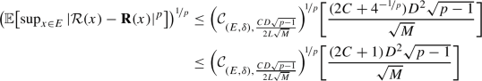 (5.14)

(cf. Definition 4.7).
Proof of Lemma 5.6
Throughout this proof, let \( {\mathcal {Y}}_{ x, j } :\Omega \rightarrow {\mathbb {R}}\), \( j \in \{ 1, 2, \ldots , M \} \), \( x \in E \), satisfy for all \( x \in E \), \( j \in \{ 1, 2, \ldots , M \} \) that \( {\mathcal {Y}}_{ x, j } = \left| X_{ x, j } - Y_j \right|^2 \). Observe that the assumption that \(\forall \, x \in E, \, j \in \{ 1, 2, \ldots , M \} :\left| X_{ x, j } - Y_j \right| \le D \) shows for all \( x \in E \), \( j \in \{ 1, 2, \ldots , M \} \) that \(0 \le {\mathcal {Y}}_{x,j} \le D^2\). Corollary 5.5 therefore implies for all \(x \in E\), \(j \in \{1,2, \ldots , M\}\) that
The rest of the proof is identical to the proof of [21, Lemma 4.13], the only difference being that we apply the improved Monte Carlo estimate Corollary 5.3 instead of [21, Corollary 4.5]. The proof of Lemma 5.6 is thus complete. \(\square \)
Proposition 5.7
Let \( d, {\textbf {d}} , M \in {\mathbb {N}}\), \( L, D, p \in ( 0, \infty ) \), \( \alpha \in {\mathbb {R}}\), \( \beta \in ( \alpha , \infty ) \), \( {\mathscr {D}}\subseteq {\mathbb {R}}^d \), let \( ( \Omega , {\mathcal {F}}, {\mathbb {P}}) \) be a probability space, let \( (X_j, Y_j) :\Omega \rightarrow {\mathscr {D}}\times {\mathbb {R}}\), \( j \in \{ 1, 2, \ldots , M \} \), be i.i.d. random variables, let \( H = ( H_\theta )_{ \theta \in [ \alpha , \beta ]^{\textbf {d}} } :[ \alpha , \beta ]^{\textbf {d}} \rightarrow C( {\mathscr {D}}, {\mathbb {R}}) \) be a function, assume for all \( \theta , \vartheta \in [ \alpha , \beta ]^{\textbf {d}} \), \( j \in \{ 1, 2, \ldots , M \} \), \( x \in {\mathscr {D}}\) that \( \left| H_\theta ( X_j ) - Y_j \right| \le D \) and \( \left| H_\theta ( x ) - H_\vartheta ( x ) \right| \le L \left\Vert \theta - \vartheta \right\Vert _\infty \), let \( {\textbf {R}} :[ \alpha , \beta ]^{\textbf {d}} \rightarrow [ 0, \infty ) \) satisfy for all \( \theta \in [ \alpha , \beta ]^{\textbf {d}} \) that \( {\textbf {R}} ( \theta ) = {\mathbb {E}}[ \left| H_\theta ( X_1 ) - Y_1 \right|^2 ] \), and let \( {\mathcal {R}}:[ \alpha , \beta ]^{\textbf {d}} \times \Omega \rightarrow [ 0, \infty ) \) satisfy for all \( \theta \in [ \alpha , \beta ]^{\textbf {d}} \), \( \omega \in \Omega \) that
(cf. Definition 3.1). Then,
-
(i)
the function \( \Omega \ni \omega \mapsto \sup \nolimits _{ \theta \in [ \alpha , \beta ]^{\textbf {d}} } \left| {\mathcal {R}}( \theta , \omega ) - {\textbf {R}} ( \theta ) \right| \in [ 0, \infty ] \) is measurable and
-
(ii)
it holds that
$$\begin{aligned}{} & {} \bigl ( {\mathbb {E}}\bigl [ \sup \nolimits _{ \theta \in [ \alpha , \beta ]^{\textbf {d}} } \left| {\mathcal {R}}( \theta ) - {\textbf {R}} ( \theta ) \right| ^p \bigr ] \bigr )^{ \nicefrac {1}{p} }\nonumber \\{} & {} \quad \le \frac{2 D^2 \sqrt{ e \max \{ p, 1, {\textbf {d}} \ln ( 16 M L^2 ( \beta - \alpha )^2 D ^{ -2 } ) \} } }{ \sqrt{M} }. \end{aligned}$$(5.17)
Proof of Proposition 5.7
Analogously to the proof of [21, Proposition 4.14], one can show that Lemma 5.6 implies that the function \( \Omega \ni \omega \mapsto \sup \nolimits _{ \theta \in [ \alpha , \beta ]^{\textbf {d}} } \left| {\mathcal {R}}( \theta , \omega ) - {\textbf {R}} ( \theta ) \right| \in [ 0, \infty ] \) is measurable and

The proof of Proposition 5.7 is thus complete. \(\square \)
Corollary 5.8
Let \( d, {\textbf {d}} , {\textbf {L}} , M \in {\mathbb {N}}\), \( \beta , c \in [ 1, \infty ) \), \(p \in (0, \infty )\), \( u \in {\mathbb {R}}\), \( v \in [ u + 1, \infty ) \), \( {\textbf {l}} = ( {\textbf {l}} _0, {\textbf {l}} _1, \ldots , {\textbf {l}} _{\textbf {L}} ) \in {\mathbb {N}}^{ {\textbf {L}} + 1 } \), \( {\mathscr {D}}\subseteq [ -c, c ]^d \), assume \( {\textbf {l}} _0 = d \), \( {\textbf {l}} _{\textbf {L}} = 1 \), and \( {\textbf {d}} \ge \sum _{i=1}^{{\textbf {L}} } {\textbf {l}} _i( {\textbf {l}} _{ i - 1 } + 1 ) \), let \( ( \Omega , {\mathcal {F}}, {\mathbb {P}}) \) be a probability space, let \( (X_j,Y_j) :\Omega \rightarrow {\mathscr {D}}\times [u,v] \), \(j \in \{1,2, \ldots , M\}\), be i.i.d. random variables, let \( {\textbf {R}} :[ -\beta , \beta ]^{\textbf {d}} \rightarrow [ 0, \infty ) \) satisfy for all \( \theta \in [ -\beta , \beta ]^{\textbf {d}} \) that \( {\textbf {R}} ( \theta ) = {\mathbb {E}}\bigl [ \left| {\mathscr {N}}^{\theta , {\textbf {l}} }_{u,v}( X_1 ) - Y_1 \right|^2 \bigr ] \), and let \( {\mathcal {R}}:[ -\beta , \beta ]^{\textbf {d}} \times \Omega \rightarrow [ 0, \infty ) \) satisfy for all \( \theta \in [ -\beta , \beta ]^{\textbf {d}} \), \( \omega \in \Omega \) that
(cf. Definition 2.8). Then,
-
(i)
the function \( \Omega \ni \omega \mapsto \sup \nolimits _{ \theta \in [ -\beta , \beta ]^{\textbf {d}} } \left| {\mathcal {R}}( \theta , \omega ) - {\textbf {R}} ( \theta ) \right| \in [ 0, \infty ] \) is measurable and
-
(ii)
it holds that
 (5.20)

(cf. Definition 3.1).
Proof of Corollary 5.8
Throughout this proof let \( L \in ( 0, \infty ) \) be given by \( L = c {\textbf {L}} ( \left\Vert {\textbf {l}} \right\Vert _\infty + 1 )^{\textbf {L}} \beta ^{ {\textbf {L}} - 1 } \). Using the same arguments as in the proof of [21, Corollary 4.15], we obtain from [4, Corollary 2.37] and Proposition 5.7 that the function \( \Omega \ni \omega \mapsto \sup \nolimits _{ \theta \in [ -\beta , \beta ]^{\textbf {d}} } \left| {\mathcal {R}}( \theta , \omega ) - {\textbf {R}} ( \theta ) \right| \in [ 0, \infty ] \) is measurable and
This, the fact that \( 64 {\textbf {L}} ^2 \le 2^6 2^{ 2 ( {\textbf {L}} - 1 ) } = 2^{ 4 + 2 {\textbf {L}} } \le 2^{ 4 {\textbf {L}} + 2 {\textbf {L}} } = 2^{ 6 {\textbf {L}} } \), and the facts that \( \sqrt{2e} < \tfrac{5}{2} \), \( \beta \ge 1 \), \( {\textbf {L}} \ge 1 \), \( M \ge 1 \), and \( c \ge 1 \) show that

In addition, the facts that \(\left\Vert {\textbf {l}} \right\Vert _{ \infty } \ge 1\) and \( \forall \, n \in {\mathbb {N}}:n \le 2^{ n - 1 }\) imply that
This demonstrates that

Combining this and (5.22) completes the proof of Corollary 5.8. \(\square \)
6 Overall Error Analysis
In this section, we combine the upper bounds for the approximation error and for the generalization error with the results for the optimization error from [21] to obtain strong overall error estimates for the training of DNNs. The two main results of this section are Theorem 6.2 and Theorem 6.6 which estimate the overall error in the case of one-dimensional and multidimensional input data, respectively. In both cases, the random variables \(\Theta _{k,n}\), \(k,n \in {\mathbb {N}}_0\), are allowed to be computed via an arbitrary optimization algorithm with i.i.d. random initializations. A central feature of Theorem 6.2 is that a single hidden layer is sufficient in order for the overall error to converge to zero reasonably fast. In Theorem 6.6, the error converges to zero exponentially with respect to the number of layers.
The two main theorems follow from the more general Proposition 6.1 in Sect. 6.1. Let us provide a few additional comments regarding the mathematical objects appearing in Proposition 6.1 and subsequent results. The vector \({\textbf {l}} \in {\mathbb {N}}^{{\textbf {L}} + 1}\) determines the architecture of a DNN with input dimension \({\textbf {l}} _0=d\), output dimension \({\textbf {l}} _{\textbf {L}} =1\), and \({\textbf {L}} -1\) hidden layers of dimensions \({\textbf {l}} _1, {\textbf {l}} _2, \ldots , {\textbf {l}} _{{\textbf {L}} -1}\), respectively. The natural number \(d \in {\mathbb {N}}\) specifies the dimension of the input data. The target function \({\mathcal {E}}:[a,b]^d \rightarrow [u,v]\), which we intend to approximate, is assumed to be bounded and measurable. For every \(\theta \in {\mathbb {R}}^{\textbf {d}} \) the function \( {\mathscr {N}}^{\theta , {\textbf {l}} }_{u,v} :{\mathbb {R}}^d \rightarrow {\mathbb {R}}\), as introduced in Definition 2.8, is the realization of a clipped rectified DNN with parameters (weights and biases) given by the vector \(\theta \). The training samples \((X_j, Y_j)\), \(j \in \{1,2, \ldots , M\}\), are used to compute the empirical risk \({\mathcal {R}}\) in (6.1). The random variables \(\Theta _{k,n} :\Omega \rightarrow {\mathbb {R}}^{\textbf {d}} \), \(k, n \in {\mathbb {N}}_0\), are allowed to be computed via an arbitrary stochastic optimization algorithm with i.i.d. random initializations \(\Theta _{k,0}\), \(k \in \{1, 2, \ldots , K\}\), and the real number \(c \in [\max \{ 1 , |a| , |b| \} , \infty )\) quantifies the magnitude of the parameters at the initialization. The random double index \(({\textbf {k}} (\omega ) , {\textbf {n}} ( \omega ) ) \in ({\mathbb {N}}_0)^2\) is chosen in such a way that the empirical risk \({\mathcal {R}}(\Theta _{k,n})\) is minimized, where only the parameter vectors inside the hypercube \([- \beta , \beta ]^{\textbf {d}} \) are considered (cf. (6.2)).
The proof of Proposition 6.1 relies on the \(L^2\)-error decomposition [21, Proposition 6.1] (cf. [4, Lemma 4.3]), which shows that the overall error can be decomposed into the approximation error, the generalization error and the optimization error. To estimate the generalization error we use Corollary 5.8, and for the optimization error we apply the result from Jentzen & Welti [21, Corollary 5.8]. We also note that the overall \(L^2\)-error is measurable and therefore the expectation on the left-hand side of (6.12) (and similarly in subsequent results) is well defined. Proposition 6.1 is very similar to [21, Proposition 6.3], and the proof is only included for completeness.
Afterward, in Sect. 6.2 we combine this with the estimate for one-dimensional functions, Corollary 4.3, to derive Theorem 6.2. In Corollary 6.4 we state a simplified estimate where the architecture parameter A is replaced by the dimension of the single hidden layer. The proof uses the elementary Lemma 6.3, which is very similar to [21, Lemma 6.4]. Next, in Sect. 6.3 we specialize the results by assuming that the \(\Theta _{k,n}\), \(k,n \in {\mathbb {N}}_0\), are computed via stochastic gradient descent (cf. Corollary 6.5).
Thereafter, in Sect. 6.4 we combine Proposition 6.1 with the upper bound for the approximation error in the multidimensional case, Proposition 4.8, to obtain in Theorem 6.6 a strong overall error estimate. In Corollary 6.7 we replace the parameter A by the minimum of \(2^{{\textbf {L}} -1}\), where \({\textbf {L}} \) is the depth of the employed DNN, and the layer dimensions \({\textbf {l}} _1, {\textbf {l}} _2, \ldots , {\textbf {l}} _{{\textbf {L}} - 1}\). The next result, Corollary 6.8, is a simplified version of Corollary 6.7. In particular, the \(L^p\)-norm of the \(L^2\)-error is replaced by the expectation of the \(L^1\)-error and the training samples are restricted to unit hypercubes.
Finally, in Sect. 6.5 we apply the results from Sect. 6.4 to the case where the random parameter vectors \(\Theta _{k,n}\), \(k,n \in {\mathbb {N}}_0\), are again computed by stochastic gradient descent. More specifically, Corollary 6.9 specializes Corollary 6.7 to this case, and Corollary 6.10 is an immediate consequence of Corollary 6.8.
6.1 General Error Analysis for the Training of DNNs Via Random Initializations
Proposition 6.1
Let \(d, {\textbf {d}} , {\textbf {L}} , M,K,N \in {\mathbb {N}}\), \(p \in (0, \infty )\), \(a, u \in {\mathbb {R}}\), \(b \in (a, \infty )\), \(v \in (u, \infty )\), \(c \in [ \max \{1, |a|, |b| \}, \infty )\), \(\beta \in [c, \infty )\), \({\textbf {l}} = ({\textbf {l}} _0, {\textbf {l}} _1, \ldots , {\textbf {l}} _{\textbf {L}} ) \in {\mathbb {N}}^{{\textbf {L}} +1}\), \({\mathfrak {N}}\subseteq \{0,1,\ldots , N\}\) satisfy \(0 \in {\mathfrak {N}}\), \({\textbf {l}} _0=d\), \({\textbf {l}} _{\textbf {L}} = 1\), and \({\textbf {d}} \ge \sum _{i=1}^{\textbf {L}} {\textbf {l}} _i({\textbf {l}} _{i-1}+1)\), let \((\Omega , {\mathcal {F}}, {\mathbb {P}})\) be a probability space, let \((X_j, Y_j) :\Omega \rightarrow [a,b]^d \times [u,v]\), \(j \in \{1,2, \ldots , M\}\), be i.i.d. random variables, let \({\mathcal {E}}:[a,b]^d \rightarrow [u,v]\) be a measurable function, assume that it holds \({\mathbb {P}}\)-a.s. that \({\mathcal {E}}(X_1) = {\mathbb {E}}[Y_1|X_1]\), let \({\textbf {k}} :\Omega \rightarrow {\mathbb {N}}_0\), \({\textbf {n}} :\Omega \rightarrow {\mathbb {N}}_0\), and \(\Theta _{k, n} :\Omega \rightarrow {\mathbb {R}}^{\textbf {d}} \), \(k, n \in {\mathbb {N}}_0\), be random variables, assume that \(\Theta _{k,0}\), \(k \in \{1,2, \ldots , K\}\), are i.i.d., assume that \(\Theta _{1,0}\) is continuous uniformly distributed on \([-c,c]^{\textbf {d}} \), and let \({\mathcal {R}}:{\mathbb {R}}^{\textbf {d}} \times \Omega \rightarrow [0, \infty )\) satisfy for all \(\theta \in {\mathbb {R}}^{\textbf {d}} \), \(\omega \in \Omega \) that
(cf. Definitions 2.8 and 3.1). Then,
-
(i)
the function
$$\begin{aligned} \Omega \ni \omega \mapsto \int _{[a,b]^d} \bigl | {\mathscr {N}}^{\Theta _{{\textbf {k}} (\omega ) , {\textbf {n}} ( \omega )}(\omega ), {\textbf {l}} }_{u,v} (x)-{\mathcal {E}}(x) \bigr | ^2 \, {\mathbb {P}}_{X_1}(\text {d} x) \in [0, \infty ] \end{aligned}$$(6.3)is measurable and
-
(ii)
it holds that
 (6.4)
(6.4)

Proof of Proposition 6.1
Observe that item (i) follows from [21, Lemma 6.2 (iii)] (applied with \(D \curvearrowleft [a,b]^d \), \(X \curvearrowleft X_1\), \(p \curvearrowleft 2\) in the notation of [21, Lemma 6.2]). To prove (ii), let \({\textbf {R}} :{\mathbb {R}}^{\textbf {d}} \rightarrow [0, \infty )\) satisfy for all \(\theta \in {\mathbb {R}}^{\textbf {d}} \) that \({\textbf {R}} (\theta ) = {\mathbb {E}}| {\mathscr {N}}^{\theta , {\textbf {l}} }_{u,v}(X_1)-Y_1|^2\). The assumptions that \(\Theta _{k,0}\), \(k \in \{1,2, \ldots , K\}\) are continuous uniformly distributed on \([-c, c]^{\textbf {d}} \) and \(\beta \ge c\) ensure that \({\mathbb {P}}\)-a.s. we have that \(\left( \bigcup _{k=1}^K \Theta _{k,0}(\Omega ) \right) \subseteq [-\beta ,\beta ]^{\textbf {d}} \). This, the fact that \(0 \in {\mathfrak {N}}\), and the \(L^2\)-error decomposition [21, Proposition 6.1] show that for all \(\vartheta \in [-\beta ,\beta ]^{\textbf {d}} \), it holds \({\mathbb {P}}\)-a.s. that

Combining this and Minkowski’s inequality demonstrates for all \(q \in [1, \infty )\), \(\vartheta \in [-c,c]^{\textbf {d}} \) that

Next, observe that the fact that \([a,b]^d \subseteq [-c, c ]^d\) and Corollary 5.8 (applied with \( {\mathscr {D}}\curvearrowleft [a,b]^d\), \(v \curvearrowleft \max \{u+1, v\}\), \(p \curvearrowleft q\) in the notation of Corollary 5.8) imply for all \(q \in (0, \infty )\) that

Moreover, [21, Corollary 5.8] (applied with \(D \curvearrowleft [a,b]^d\), \(b \curvearrowleft c\), \(\beta \curvearrowleft c\), \((\Theta _k)_{k \in \{1, \ldots , K\}} \curvearrowleft (\Theta _{k,0})_{k \in \{1, \ldots , K \} }\), \(p \curvearrowleft q\) in the notation of [21, Corollary 5.8]) proves for all \(q \in (0, \infty )\) that

Combining (6.6)–(6.8) with Jensen’s inequality and the fact that \(\ln (4 M \beta c) \ge 1\) demonstrates that

This completes the proof of Proposition 6.1. \(\square \)
6.2 One-Dimensional Strong Overall Error Analysis
Theorem 6.2
Let \({\textbf {d}} , {\textbf {L}} , M,K,N \in {\mathbb {N}}\), \(A, p \in (0, \infty )\), \(L \in [0, \infty )\), \(a, u \in {\mathbb {R}}\), \(v \in (u, \infty )\), \(b \in (a, \infty )\), \(c \in [ \max \{1, |u|, |v|, |a|, |b|, 2L \}, \infty )\), \(\beta \in [c, \infty )\), \({\textbf {l}} = ({\textbf {l}} _0, {\textbf {l}} _1, \ldots , {\textbf {l}} _{\textbf {L}} ) \in {\mathbb {N}}^{{\textbf {L}} +1}\), \({\mathfrak {N}}\subseteq \{0,1,\ldots , N\}\) satisfy \(0 \in {\mathfrak {N}}\), \( {\textbf {L}} \ge 2 \), \( {\textbf {l}} _0 = {\textbf {l}} _{\textbf {L}} =1 \), \( {\textbf {l}} _1 \ge A +2 \), and \( {\textbf {d}} \ge \sum _{i=1}^{{\textbf {L}} } {\textbf {l}} _i( {\textbf {l}} _{ i - 1 } + 1 ) \), assume for all \( i \in \{ 2, 3, \ldots , {\textbf {L}} -1\}\) that \( {\textbf {l}} _i \ge 2\), let \((\Omega , {\mathcal {F}}, {\mathbb {P}})\) be a probability space, let \((X_j, Y_j) :\Omega \rightarrow [a,b] \times [u,v]\), \(j \in \{1,2, \ldots , M\}\), be i.i.d. random variables, let \({\mathcal {E}}:[a,b] \rightarrow [u,v]\) satisfy \({\mathbb {P}}\)-a.s. that \({\mathcal {E}}(X_1) = {\mathbb {E}}[Y_1|X_1]\), assume for all \(x,y \in [a,b]\) that \(|{\mathcal {E}}(x)- {\mathcal {E}}(y)| \le L |x-y|\), let \({\textbf {k}} :\Omega \rightarrow {\mathbb {N}}_0\), \({\textbf {n}} :\Omega \rightarrow {\mathbb {N}}_0\), and \(\Theta _{k, n} :\Omega \rightarrow {\mathbb {R}}^{\textbf {d}} \), \(k, n \in {\mathbb {N}}_0\), be random variables, assume that \(\Theta _{k,0}\), \(k \in \{1,2, \ldots , K\}\), are i.i.d., assume that \(\Theta _{1,0}\) is continuous uniformly distributed on \([-c,c]^{\textbf {d}} \), and let \({\mathcal {R}}:{\mathbb {R}}^{\textbf {d}} \times \Omega \rightarrow [0, \infty )\) satisfy for all \(\theta \in {\mathbb {R}}^{\textbf {d}} \), \(\omega \in \Omega \) that
(cf. Definitions 2.8 and 3.1). Then,

Proof of Theorem 6.2
First of all, note that Proposition 6.1 proves that

Furthermore, observe that Corollary 4.3 ensures that there exists \(\vartheta \in {\mathbb {R}}^{\textbf {d}} \) such that \(\left\Vert \vartheta \right\Vert _\infty \le \max \{1, 2L, |a|, |b|, 2\sup \nolimits _{x \in [a,b]} |{\mathcal {E}}(x)| \}\) and
The assumption that \({\mathcal {E}}([a,b]) \subseteq [u,v]\) implies that \(\sup \nolimits _{x \in [a,b]} |{\mathcal {E}}(x)| \le \max \{|u|, |v|\} \le c\) and thus \(\left\Vert \vartheta \right\Vert _\infty \le c\). Equation (6.14) therefore demonstrates that
Combining this and (6.13) completes the proof of Theorem 6.2. \(\square \)
Lemma 6.3
Let \(c, M \in [1, \infty )\) and \(\beta \in [c, \infty )\). Then, it holds that
Proof of Lemma 6.3
First, observe that the fact that \(\forall \, y \in {\mathbb {R}}:e^{y-1} \ge y\) implies that
This, the assumption that \(\beta \ge c\), and the facts that \(\tfrac{4\beta }{e} > 1\), \(\ln (M) \ge 0\), and \(\tfrac{4}{e} < \tfrac{3}{2}\) demonstrate that

The proof of Lemma 6.3 is thus complete. \(\square \)
Corollary 6.4
Let \({\textbf {d}} , M,K,N \in {\mathbb {N}}\), \(p \in (0, \infty )\), \( L \in [0, \infty )\), \(a, u \in {\mathbb {R}}\), \(v \in (u, \infty )\), \(b \in (a, \infty )\), \(c \in [ \max \{1, 2|u|, 2|v|, |a|, |b|, 2L \}, \infty )\), \(\beta \in [c, \infty )\), \(\ell \in {\mathbb {N}}\cap [3, \infty ) \cap (0, \nicefrac {({\textbf {d}} - 1)}{3}]\), let \({\mathfrak {N}}\subseteq \{0,1,\ldots , N\}\) satisfy \(0 \in {\mathfrak {N}}\), let \((\Omega , {\mathcal {F}}, {\mathbb {P}})\) be a probability space, let \((X_j, Y_j) :\Omega \rightarrow [a,b] \times [u,v]\), \(j \in \{1,2, \ldots , M\}\), be i.i.d. random variables, let \({\mathcal {E}}:[a,b] \rightarrow [u,v]\) satisfy \({\mathbb {P}}\)-a.s. that \({\mathcal {E}}(X_1) = {\mathbb {E}}[Y_1|X_1]\), assume for all \(x,y \in [a,b]\) that \(| {\mathcal {E}}(x)- {\mathcal {E}}(y)| \le L |x-y|\), let \({\textbf {k}} :\Omega \rightarrow {\mathbb {N}}_0\), \({\textbf {n}} :\Omega \rightarrow {\mathbb {N}}_0\), and \(\Theta _{k, n} :\Omega \rightarrow {\mathbb {R}}^{\textbf {d}} \), \(k, n \in {\mathbb {N}}_0\), be random variables, assume that \(\Theta _{k,0}\), \(k \in \{1,2, \ldots , K\}\), are i.i.d., assume that \(\Theta _{1,0}\) is continuous uniformly distributed on \([-c,c]^{\textbf {d}} \), and let \({\mathcal {R}}:{\mathbb {R}}^{\textbf {d}} \times \Omega \rightarrow [0, \infty )\) satisfy for all \(\theta \in {\mathbb {R}}^{\textbf {d}} \), \(\omega \in \Omega \) that
(cf. Definitions 2.8 and 3.1). Then,

Proof of Corollary 6.4
Observe that the assumption that \({\textbf {d}} \ge 3 \ell +1\) and Theorem 6.2 (applied with \({\textbf {L}} \curvearrowleft 2\), \({\textbf {l}} \curvearrowleft (1, \ell , 1)\), \(A \curvearrowleft \ell -2\), \(p \curvearrowleft \nicefrac {p}{2}\) in the notation of Theorem 6.2) demonstrate that
Combining this, Lemma 6.3, and the facts that \(c \ge |u|+|v| \ge |u-v|\), \(L \le \frac{c}{2}\), and \(|b-a| \le 2c\) shows that

Furthermore, the fact that \(\ell \in \{3,4,5, \ldots \}\) implies that \(\ell ^4 \ge 3 \ell ^3 > \tfrac{4^3}{3^3} \ell ^3 = \left( \tfrac{4 \ell }{3} \right) ^3 \ge ( \ell +1)^3\), \(4 \ell = 3 \ell + \ell > \sqrt{8} \, \ell + \sqrt{8} = \sqrt{8}( \ell +1)\), and \(3( \ell -2) \ge \ell \) and therefore

This completes the proof of Corollary 6.4. \(\square \)
6.3 Stochastic Gradient Descent for One-Dimensional Target Functions
Corollary 6.5
Let \({\textbf {d}} , M,K,N \in {\mathbb {N}}\), \(p \in (0, \infty )\), \( L \in [0, \infty )\), \(a, u \in {\mathbb {R}}\), \(v \in (u, \infty )\), \(b \in (a, \infty )\), \(c \in [ \max \{1, 2|u|, 2|v|, |a|, |b|, 2L \}, \infty )\), \(\beta \in [c, \infty )\), \((\gamma _n)_{n \in {\mathbb {N}}} \subseteq {\mathbb {R}}\), \((J_n)_{n \in {\mathbb {N}}} \subseteq {\mathbb {N}}\), \(\ell \in {\mathbb {N}}\cap [3, \infty ) \cap (0, \nicefrac {({\textbf {d}} - 1)}{3}]\), let \({\mathfrak {N}}\subseteq \{0,1,\ldots , N\}\) satisfy \(0 \in {\mathfrak {N}}\), let \((\Omega , {\mathcal {F}}, {\mathbb {P}})\) be a probability space, let \((X_j^{k,n}, Y_j^{k,n}) :\Omega \rightarrow [a,b] \times [u,v]\), \(j \in {\mathbb {N}}\), \(k,n \in {\mathbb {N}}_0\), be random variables, assume that \((X_j^{0,0}, Y_j^{0,0})\), \(j \in \{1,2, \ldots , M\}\), are i.i.d., let \({\mathcal {E}}:[a,b] \rightarrow [u,v]\) satisfy \({\mathbb {P}}\)-a.s. that \({\mathcal {E}}(X_1^{0,0}) = {\mathbb {E}}[Y_1^{0,0}|X_1^{0,0}]\), assume for all \(x,y \in [a,b]\) that \(| {\mathcal {E}}(x)- {\mathcal {E}}(y)| \le L |x-y|\), let \({\textbf {k}} :\Omega \rightarrow {\mathbb {N}}_0\), \({\textbf {n}} :\Omega \rightarrow {\mathbb {N}}_0\), and \(\Theta _{k, n} :\Omega \rightarrow {\mathbb {R}}^{\textbf {d}} \), \(k, n \in {\mathbb {N}}_0\), be random variables, assume that \(\Theta _{k,0}\), \(k \in \{1,2, \ldots , K\}\), are i.i.d., assume that \(\Theta _{1,0}\) is continuous uniformly distributed on \([-c,c]^{\textbf {d}} \), let \({\mathcal {R}}_J^{k,n} :{\mathbb {R}}^{\textbf {d}} \times \Omega \rightarrow [0, \infty )\) satisfy for all \(J \in {\mathbb {N}}\), \(k,n \in {\mathbb {N}}_0\), \(\theta \in {\mathbb {R}}^{\textbf {d}} \), \(\omega \in \Omega \) that
let \({\mathcal {G}}^{k,n} :{\mathbb {R}}^{\textbf {d}} \times \Omega \rightarrow {\mathbb {R}}^{\textbf {d}} \), \(k,n\in {\mathbb {N}}\), satisfy for all \( k,n \in {\mathbb {N}}\), \(\omega \in \Omega \), \(\theta \in \{ \vartheta \in {\mathbb {R}}^{\textbf {d}} :({\mathcal {R}}^{k,n}_{J_n}(\cdot , \omega ) :{\mathbb {R}}^{\textbf {d}} \rightarrow [0, \infty ) \text { is differentiable at } \vartheta )\}\) that \({\mathcal {G}}^{k,n}(\theta , \omega ) = (\nabla _\theta {\mathcal {R}}^{k,n}_{J_n})(\theta , \omega )\), assume for all \( k,n \in {\mathbb {N}}\) that \(\Theta _{k,n} = \Theta _{k, n-1} - \gamma _n {\mathcal {G}}^{k,n}(\Theta _{k, n-1})\), and assume for all \(\omega \in \Omega \) that
(cf. Definitions 2.8 and 3.1). Then,

Proof of Corollary 6.5
This is a direct consequence of Corollary 6.4 (applied with \({\mathcal {R}}\curvearrowleft {\mathcal {R}}_M^{0,0}\), \(((X_j, Y_j))_{j \in \{1, \ldots , M \} } \curvearrowleft ((X_j^{0,0}, Y_j^{0,0}))_{j \in \{1, \ldots , M \} }\) in the notation of Corollary 6.4). The proof of Corollary 6.5 is thus complete. \(\square \)
6.4 Multidimensional Strong Overall Error Analysis
Theorem 6.6
Let \(d, {\textbf {d}} , {\textbf {L}} , M,K,N \in {\mathbb {N}}\), \(A, p \in (0, \infty )\), \(L \in [ 0, \infty )\), \(a, u \in {\mathbb {R}}\), \(v \in (u, \infty )\), \(b \in (a, \infty )\), \(c \in [ \max \{1, 2|u|, 2|v|, |a|, |b|, L \}, \infty )\), \(\beta \in [c, \infty )\), \({\textbf {l}} = ({\textbf {l}} _0, {\textbf {l}} _1, \ldots , {\textbf {l}} _{\textbf {L}} ) \in {\mathbb {N}}^{{\textbf {L}} +1}\), let \({\mathfrak {N}}\subseteq \{0,1,\ldots , N\}\) satisfy \(0 \in {\mathfrak {N}}\), assume  , \({\textbf {l}} _0 = d \),
  , \( {\textbf {l}} _{\textbf {L}} = 1 \), and \( {\textbf {d}} \ge \sum _{i=1}^{{\textbf {L}} } {\textbf {l}} _i( {\textbf {l}} _{ i - 1 } + 1 ) \), assume for all \( i \in \{ 2, 3, \ldots , {\textbf {L}} -1\}\) that
  , let \((\Omega , {\mathcal {F}}, {\mathbb {P}})\) be a probability space, let \((X_j, Y_j) :\Omega \rightarrow [a,b]^d \times [u,v]\), \(j \in \{1,2, \ldots , M\}\), be i.i.d. random variables, let \({\mathcal {E}}:[a,b]^d \rightarrow [u,v]\) satisfy \({\mathbb {P}}\)-a.s. that \({\mathcal {E}}(X_1) = {\mathbb {E}}[Y_1|X_1]\), assume for all \(x,y \in [a,b]^d\) that \(| {\mathcal {E}}(x)- {\mathcal {E}}(y)| \le L \left\Vert x-y \right\Vert _1\), let \({\textbf {k}} :\Omega \rightarrow {\mathbb {N}}_0\), \({\textbf {n}} :\Omega \rightarrow {\mathbb {N}}_0\), and \(\Theta _{k, n} :\Omega \rightarrow {\mathbb {R}}^{\textbf {d}} \), \(k, n \in {\mathbb {N}}_0\), be random variables, assume that \(\Theta _{k,0}\), \(k \in \{1,2, \ldots , K\}\), are i.i.d., assume that \(\Theta _{1,0}\) is continuous uniformly distributed on \([-c,c]^{\textbf {d}} \), and let \({\mathcal {R}}:{\mathbb {R}}^{\textbf {d}} \times \Omega \rightarrow [0, \infty )\) satisfy for all \(\theta \in {\mathbb {R}}^{\textbf {d}} \), \(\omega \in \Omega \) that
(cf. Definitions 2.8, 3.1, and 3.9). Then,

Proof of Theorem 6.6
Observe that Proposition 4.8 ensures that there exists \(\vartheta \in {\mathbb {R}}^{\textbf {d}} \) such that \(\left\Vert \vartheta \right\Vert _\infty \le \max \{1, L, |a|, |b|, 2\sup \nolimits _{x \in [a,b]^d} |{\mathcal {E}}(x)| \}\) and
The assumption that \({\mathcal {E}}([a,b]^d) \subseteq [u,v]\) implies that \(\sup \nolimits _{x \in [a,b]^d} |{\mathcal {E}}(x)| \le \max \{|u|, |v|\} \le \frac{c}{2}\) and thus \(\left\Vert \vartheta \right\Vert _\infty \le c\). Equation (6.31) therefore shows that
Combining this with Proposition 6.1 establishes (6.30) and thus completes the proof of Theorem 6.6. \(\square \)
Corollary 6.7
Let \(d, {\textbf {d}} , {\textbf {L}} , M,K,N \in {\mathbb {N}}\), \(p \in (0, \infty )\), \( L \in [0, \infty )\), \(a, u \in {\mathbb {R}}\), \(v \in (u, \infty )\), \(b \in (a, \infty )\), \(c \in [ \max \{1, 2|u|, 2|v|, |a|, |b|, L \}, \infty )\), \(\beta \in [c, \infty )\), \({\textbf {l}} = ({\textbf {l}} _0, {\textbf {l}} _1, \ldots , {\textbf {l}} _{\textbf {L}} ) \in {\mathbb {N}}^{{\textbf {L}} +1}\), \({\mathfrak {N}}\subseteq \{0,1,\ldots , N\}\) satisfy \(0 \in {\mathfrak {N}}\), \( {\textbf {l}} _0 = d \), \( {\textbf {l}} _{\textbf {L}} = 1 \), and \( {\textbf {d}} \ge \sum _{i=1}^{{\textbf {L}} } {\textbf {l}} _i( {\textbf {l}} _{ i - 1 } + 1 ) \), let \((\Omega , {\mathcal {F}}, {\mathbb {P}})\) be a probability space, let \((X_j, Y_j) :\Omega \rightarrow [a,b]^d \times [u,v]\), \(j \in \{1,2, \ldots , M\}\), be i.i.d. random variables, let \({\mathcal {E}}:[a,b]^d \rightarrow [u,v]\) satisfy \({\mathbb {P}}\)-a.s. that \({\mathcal {E}}(X_1) = {\mathbb {E}}[Y_1|X_1]\), assume for all \(x,y \in [a,b]^d\) that \(| {\mathcal {E}}(x)- {\mathcal {E}}(y)| \le L \left\Vert x-y \right\Vert _1\), let \({\textbf {k}} :\Omega \rightarrow {\mathbb {N}}_0\), \({\textbf {n}} :\Omega \rightarrow {\mathbb {N}}_0\), and \(\Theta _{k, n} :\Omega \rightarrow {\mathbb {R}}^{\textbf {d}} \), \(k, n \in {\mathbb {N}}_0\), be random variables, assume that \(\Theta _{k,0}\), \(k \in \{1,2, \ldots , K\}\), are i.i.d., assume that \(\Theta _{1,0}\) is continuous uniformly distributed on \([-c,c]^{\textbf {d}} \), and let \({\mathcal {R}}:{\mathbb {R}}^{\textbf {d}} \times \Omega \rightarrow [0, \infty )\) satisfy for all \(\theta \in {\mathbb {R}}^{\textbf {d}} \), \(\omega \in \Omega \) that
(cf. Definitions 2.8, 3.1 and 3.9). Then,

Proof of Corollary 6.7
Throughout this proof, let \(A \in {\mathbb {N}}\) be given by
Note that the assumption that \({\textbf {l}} _{\textbf {L}} =1\) shows that

Moreover, observe that

(cf. Definition 3.9). Furthermore, note that the facts that \(A \in {\mathbb {N}}\) and \(d \ge 1\) imply for all \(i \in \{2,3, \ldots , {\textbf {L}} -1 \}\) that

Combining Corollarys (6.37) and (6.39), the assumptions that \({\textbf {l}} _0=d\), \({\textbf {l}} _{\textbf {L}} =1\), and Theorem 6.6 (applied with \(p \curvearrowleft \nicefrac {p}{2}\) in the notation of Theorem 6.6) demonstrates that

This, (6.36), the assumptions that \(\beta \ge c \ge 1\), \(M \ge 1\), \(c \ge |u|+|v| \ge v-u\), and Lemma 6.3 imply that

This completes the proof of Corollary 6.7. \(\square \)
Corollary 6.8
Let \(d, {\textbf {d}} , {\textbf {L}} , M,K, N \in {\mathbb {N}}\), \(c \in [2,\infty )\), \({\textbf {l}} = ({\textbf {l}} _0, {\textbf {l}} _1, \ldots , {\textbf {l}} _{\textbf {L}} ) \in {\mathbb {N}}^{{\textbf {L}} +1}\), \({\mathfrak {N}}\subseteq \{0,1,\ldots , N\}\) satisfy \(0 \in {\mathfrak {N}}\), \( {\textbf {l}} _0 = d \), \( {\textbf {l}} _{\textbf {L}} = 1 \), and \( {\textbf {d}} \ge \sum _{i=1}^{{\textbf {L}} } {\textbf {l}} _i( {\textbf {l}} _{ i - 1 } + 1 ) \), let \((\Omega , {\mathcal {F}}, {\mathbb {P}})\) be a probability space, let \((X_j, Y_j) :\Omega \rightarrow [0,1]^d \times [0,1]\), \(j \in \{1,2, \ldots , M\}\), be i.i.d. random variables, let \({\mathcal {E}}:[0,1]^d \rightarrow [0,1]\) satisfy \({\mathbb {P}}\)-a.s. that \({\mathcal {E}}(X_1) = {\mathbb {E}}[Y_1|X_1]\), assume for all \(x,y \in [0,1]^d\) that \(|{\mathcal {E}}(x)- {\mathcal {E}}(y)| \le c \left\Vert x-y \right\Vert _1\), let \({\textbf {k}} :\Omega \rightarrow {\mathbb {N}}_0\), \({\textbf {n}} :\Omega \rightarrow {\mathbb {N}}_0\), and \(\Theta _{k, n} :\Omega \rightarrow {\mathbb {R}}^{\textbf {d}} \), \(k, n \in {\mathbb {N}}_0\), be random variables, assume that \(\Theta _{k, 0}\), \(k \in \{1,2, \ldots , K\}\), are i.i.d., assume that \(\Theta _{1, 0}\) is continuous uniformly distributed on \([-c,c]^{\textbf {d}} \), and let \({\mathcal {R}}:{\mathbb {R}}^{\textbf {d}} \times \Omega \rightarrow [0, \infty )\) satisfy for all \(\theta \in {\mathbb {R}}^{\textbf {d}} \), \(\omega \in \Omega \) that
(cf. Definitions 2.8 and 3.1). Then,

Proof of Corollary 6.8
Observe that Jensen’s inequality implies that
Combining this, the facts that \(\Vert {\textbf {l}} \Vert _\infty \ge 1\), \(c \ge 2\), \({\textbf {L}} \ge 1\), and Corollary 6.7 (applied with \(a \curvearrowleft 0\), \(b \curvearrowleft 1\), \(u \curvearrowleft 0\), \(v \curvearrowleft 1\), \(\beta \curvearrowleft c\), \(L \curvearrowleft c\), \(p \curvearrowleft 1\) in the notation of Corollary 6.7) establishes (6.44). The proof of Corollary 6.8 is thus complete. \(\square \)
6.5 Stochastic Gradient Descent for Multidimensional Target Functions
Corollary 6.9
Let \(d, {\textbf {d}} , {\textbf {L}} , M,K,N \in {\mathbb {N}}\), \(p \in (0, \infty )\), \( L \in [0, \infty )\), \(a, u \in {\mathbb {R}}\), \(v \in (u, \infty )\), \(b \in (a, \infty )\), \(c \in [ \max \{1, 2|u|, 2|v|, |a|, |b|, L \}, \infty )\), \(\beta \in [c, \infty )\), \((\gamma _n) _{n \in {\mathbb {N}}} \subseteq {\mathbb {R}}\), \((J_n)_{n \in {\mathbb {N}}} \subseteq {\mathbb {N}}\), \({\textbf {l}} = ({\textbf {l}} _0, {\textbf {l}} _1, \ldots , {\textbf {l}} _{\textbf {L}} ) \in {\mathbb {N}}^{{\textbf {L}} +1}\), \({\mathfrak {N}}\subseteq \{0,1,\ldots , N\}\) satisfy \(0 \in {\mathfrak {N}}\), \( {\textbf {l}} _0 = d \), \( {\textbf {l}} _{\textbf {L}} = 1 \), and \( {\textbf {d}} \ge \sum _{i=1}^{{\textbf {L}} } {\textbf {l}} _i( {\textbf {l}} _{ i - 1 } + 1 ) \), let \((\Omega , {\mathcal {F}}, {\mathbb {P}})\) be a probability space, let \((X_j^{k,n}, Y_j^{k,n}) :\Omega \rightarrow [a,b]^d \times [u,v]\), \(j \in {\mathbb {N}}\), \(k,n \in {\mathbb {N}}_0\), be random variables, assume that \((X_j^{0,0}, Y_j^{0,0})\), \(j \in \{1,2, \ldots , M\}\), are i.i.d., let \({\mathcal {E}}:[a,b]^d \rightarrow [u,v]\) satisfy \({\mathbb {P}}\)-a.s. that \({\mathcal {E}}(X_1^{0,0}) = {\mathbb {E}}[Y_1^{0,0}|X_1^{0,0}]\), assume for all \(x,y \in [a,b]^d\) that \(| {\mathcal {E}}(x)- {\mathcal {E}}(y)| \le L \left\Vert x-y \right\Vert _1\), let \({\textbf {k}} :\Omega \rightarrow {\mathbb {N}}_0\), \({\textbf {n}} :\Omega \rightarrow {\mathbb {N}}_0\), and \(\Theta _{k, n} :\Omega \rightarrow {\mathbb {R}}^{\textbf {d}} \), \(k, n \in {\mathbb {N}}_0\), be random variables, assume that \(\Theta _{k,0}\), \(k \in \{1,2, \ldots , K\}\), are i.i.d., assume that \(\Theta _{1,0}\) is continuous uniformly distributed on \([-c,c]^{\textbf {d}} \), let \({\mathcal {R}}^{k,n}_J :{\mathbb {R}}^{\textbf {d}} \times \Omega \rightarrow [0, \infty )\), \(J \in {\mathbb {N}}\), \(k,n \in {\mathbb {N}}_0\), satisfy for all \(J \in {\mathbb {N}}\), \(k,n \in {\mathbb {N}}_0\), \(\theta \in {\mathbb {R}}^{\textbf {d}} \), \(\omega \in \Omega \) that
let \({\mathcal {G}}^{k,n} :{\mathbb {R}}^{\textbf {d}} \times \Omega \rightarrow {\mathbb {R}}^{\textbf {d}} \), \(k,n\in {\mathbb {N}}\), satisfy for all \( k,n \in {\mathbb {N}}\), \(\omega \in \Omega \), \(\theta \in \{ \vartheta \in {\mathbb {R}}^{\textbf {d}} :({\mathcal {R}}^{k,n}_{J_n}(\cdot , \omega ) :{\mathbb {R}}^{\textbf {d}} \rightarrow [0, \infty ) \text { is differentiable at } \vartheta )\}\) that \({\mathcal {G}}^{k,n}(\theta , \omega ) = (\nabla _\theta {\mathcal {R}}^{k,n}_{J_n})(\theta , \omega )\), assume for all \( k,n \in {\mathbb {N}}\) that \(\Theta _{k,n} = \Theta _{k, n-1} - \gamma _n {\mathcal {G}}^{k,n}(\Theta _{k, n-1})\), and assume for all \(\omega \in \Omega \) that
(cf. Definitions 2.8 and 3.1). Then,

Proof of Corollary 6.9
This is a direct consequence of Corollary 6.7 (applied with \({\mathcal {R}}\curvearrowleft {\mathcal {R}}_M^{0,0}\), \(((X_j, Y_j))_{j \in \{1, \ldots , M \} } \curvearrowleft ((X_j^{0,0}, Y_j^{0,0}))_{j \in \{1, \ldots , M \} }\) in the notation of Corollary 6.7). The proof of Corollary 6.9 is thus complete. \(\square \)
Corollary 6.10
Let \(d, {\textbf {d}} , {\textbf {L}} , M, K, N \in {\mathbb {N}}\), \(c \in [2,\infty )\), \({\textbf {l}} = ({\textbf {l}} _0, {\textbf {l}} _1, \ldots , {\textbf {l}} _{\textbf {L}} ) \in {\mathbb {N}}^{{\textbf {L}} +1}\), \((\gamma _n)_{n \in {\mathbb {N}}} \subseteq {\mathbb {R}}\), \((J_n)_{n \in {\mathbb {N}}} \subseteq {\mathbb {N}}\), \({\mathfrak {N}}\subseteq \{0,1,\ldots , N\}\) satisfy \(0 \in {\mathfrak {N}}\), \( {\textbf {l}} _0 = d \), \( {\textbf {l}} _{\textbf {L}} = 1 \), and \( {\textbf {d}} \ge \sum _{i=1}^{{\textbf {L}} } {\textbf {l}} _i( {\textbf {l}} _{ i - 1 } + 1 ) \), let \((\Omega , {\mathcal {F}}, {\mathbb {P}})\) be a probability space, let \((X_j^{k,n}, Y^{k,n}_j) :\Omega \rightarrow [0,1]^d \times [0,1]\), \(j \in {\mathbb {N}}\), \(k,n \in {\mathbb {N}}_0\), be random variables, assume that \((X_j^{0,0}, Y_j^{0,0})\), \(j \in \{1,2, \ldots , M\}\), are i.i.d., let \({\mathcal {E}}:[0,1]^d \rightarrow [0,1]\) satisfy \({\mathbb {P}}\)-a.s. that \({\mathcal {E}}(X_1^{0,0}) = {\mathbb {E}}[Y_1^{0,0}|X_1^{0,0}]\), assume for all \(x,y \in [0,1]^d\) that \(|{\mathcal {E}}(x)- {\mathcal {E}}(y)| \le c \left\Vert x-y \right\Vert _1\), let \({\textbf {k}} :\Omega \rightarrow {\mathbb {N}}_0\), \({\textbf {n}} :\Omega \rightarrow {\mathbb {N}}_0\), and \(\Theta _{k, n} :\Omega \rightarrow {\mathbb {R}}^{\textbf {d}} \), \(k, n \in {\mathbb {N}}_0\), be random variables, assume that \(\Theta _{k, 0}\), \(k \in \{1,2, \ldots , K\}\), are i.i.d., assume that \(\Theta _{1, 0}\) is continuous uniformly distributed on \([-c,c]^{\textbf {d}} \), let \({\mathcal {R}}^{k,n}_J :{\mathbb {R}}^{\textbf {d}} \times \Omega \rightarrow [0, \infty )\), \(J \in {\mathbb {N}}\), \(k,n \in {\mathbb {N}}_0\), satisfy for all \(J \in {\mathbb {N}}\), \(k,n \in {\mathbb {N}}_0\), \(\theta \in {\mathbb {R}}^{\textbf {d}} \), \(\omega \in \Omega \) that
let \({\mathcal {G}}^{k,n} :{\mathbb {R}}^{\textbf {d}} \times \Omega \rightarrow {\mathbb {R}}^{\textbf {d}} \), \(k,n\in {\mathbb {N}}\), satisfy for all \( k,n \in {\mathbb {N}}\), \(\omega \in \Omega \), \(\theta \in \{ \vartheta \in {\mathbb {R}}^{\textbf {d}} :({\mathcal {R}}^{k,n}_{J_n}(\cdot , \omega ) :{\mathbb {R}}^{\textbf {d}} \rightarrow [0, \infty ) \text { is differentiable at } \vartheta )\}\) that \({\mathcal {G}}^{k,n}(\theta , \omega ) = (\nabla _\theta {\mathcal {R}}^{k,n}_{J_n})(\theta , \omega )\), assume for all \( k,n \in {\mathbb {N}}\) that \(\Theta _{k,n} = \Theta _{k, n-1} - \gamma _n {\mathcal {G}}^{k,n}(\Theta _{k, n-1})\), and assume for all \(\omega \in \Omega \) that
(cf. Definitions 2.8 and 3.1). Then,

Proof of Corollary 6.10
Observe that Corollary 6.8 (applied with \(((X_j, Y_j))_{j \in \{1, \ldots , M \} } \curvearrowleft ((X_j^{0,0}, Y_j^{0,0}))_{j \in \{1, \ldots , M \} }\), \({\mathcal {R}}\curvearrowleft {\mathcal {R}}_M^{0,0}\) in the notation of Corollary 6.8) establishes (6.51). The proof of Corollary 6.10 is thus complete. \(\square \)
References
Bach, F., Moulines, E.: Non-strongly-convex smooth stochastic approximation with convergence rate \(O(1/n)\). In: Burges, C.J.C., Bottou, L., Welling, M., Ghahramani, Z., Weinberger, K.Q. (eds.) Advances in Neural Information Processing Systems, vol. 26, pp. 773–781. Curran Associates, Inc., Red Hook (2013)
Barron, A.R.: Universal approximation bounds for superpositions of a sigmoidal function. IEEE Trans. Inf. Theory 39(3), 930–945 (1993)
Bartlett, P.L., Bousquet, O., Mendelson, S.: Local Rademacher complexities. Ann. Stat. 33(4), 1497–1537 (2005)
Beck, C., Jentzen, A., Kuckuck, B.: Full error analysis for the training of deep neural networks. Infin. Dimens. Anal. Quantum Probab. Relat. Top. 25 (2022), no. 2, Paper No. 2150020, 76 pp. 0219–0257, 65G99 (68T07), 4440215
Bercu, B., Fort, J.-C.: Generic Stochastic Gradient Methods, pp. 1–8. American Cancer Society, New York (2013)
Berner, J., Grohs, P., Jentzen, A.: Analysis of the generalization error: empirical risk minimization over deep artificial neural networks overcomes the curse of dimensionality in the numerical approximation of Black–Scholes partial differential equations. SIAM J. Math. Data Sci. 2(3), 631–657 (2020)
Cucker, F., Smale, S.: On the mathematical foundations of learning. Bull. Am. Math. Soc. (N.S.) 39(1), 1–49 (2002)
Cybenko, G.: Approximation by superpositions of a sigmoidal function. Math. Control Signals Syst. 2(4), 303–314 (1989)
Du, S.S., Zhai, X., Poczós, B., Singh, A.: Gradient descent provably optimizes over-parameterized neural networks (2018). arXiv:1810.02054
E, W., Ma, C., Wu, L.: A priori estimates of the population risk for two-layer neural networks. Commun. Math. Sci. 17(5), 1407–1425 (2019)
E, W., Ma, C., Wu, L.: A comparative analysis of optimization and generalization properties of two-layer neural network and random feature models under gradient descent dynamics. Sci. China Math. 63, 1235–1258 (2020)
Funahashi, K.-I.: On the approximate realization of continuous mappings by neural networks. Neural Netw. 2(3), 183–192 (1989)
Goodfellow, I., Bengio, Y., Courville, A.: Deep Learning. Adaptive Computation and Machine Learning. MIT Press, Cambridge, MA (2016)
Grohs, P., Hornung, F., Jentzen, A., von Wurstemberger, P.: A proof that artificial neural networks overcome the curse of dimensionality in the numerical approximation of Black-Scholes partial differential equations (2018). arXiv:1809.02362 (Accepted in Mem. Am. Math. Soc.)
Grohs, P., Hornung, F., Jentzen, A., Zimmermann, P.: Space-time error estimates for deep neural network approximations for differential equations. Adv. Comput. Math. 49 (2023), no. 1, Paper No. 4. 1019-7168, 65M99 (65M15 68T07), 4534487
Grohs, P., Jentzen, A., Salimova, D.: Deep neural network approximations for solutions of PDEs based on Monte Carlo algorithms. Partial Differ. Equ. Appl. 3 (2022), no. 4, Paper No. 45, 41 pp. 2662–2963, 65C05 (35-04), 4437476
Györfi, L., Kohler, M., Krzyżak, A., Walk, H.: A Distribution-Free Theory of Nonparametric Regression. Springer Series in Statistics. Springer, New York (2002)
Hartman, E.J., Keeler, J.D., Kowalski, J.M.: Layered neural networks with Gaussian hidden units as universal approximations. Neural Comput. 2(2), 210–215 (1990)
Hornik, K.: Approximation capabilities of multilayer feedforward networks. Neural Netw. 4(2), 251–257 (1991)
Hornik, K., Stinchcombe, M., White, H.: Multilayer feedforward networks are universal approximators. Neural Netw. 2(5), 359–366 (1989)
Jentzen, A., Welti, T.: Overall error analysis for the training of deep neural networks via stochastic gradient descent with random initialisation (2020). arXiv:2003.01291
Lu, J., Shen, Z., Yang, H., Zhang, S.: Deep network approximation for smooth functions (2020). arXiv:2001.03040
Massart, P.: Concentration Inequalities and Model Selection. Vol. 1896 of Lecture Notes in Mathematics, vol. 1896. Springer, Berlin (2007). (Lectures from the 33rd Summer School on Probability Theory held in Saint-Flour, July 6–23 (2003))
Rio, E.: Moment inequalities for sums of dependent random variables under projective conditions. J. Theor. Probab. 22, 146–163 (2009)
Shen, Z., Yang, H., Zhang, S.: Deep network approximation characterized by number of neurons (2020). arXiv:1906.05497
van de Geer, S.A.: Applications of Empirical Process Theory. Cambridge Series in Statistical and Probabilistic Mathematics, vol. 6. Cambridge University Press, Cambridge (2000)
Yarotsky, D.: Error bounds for approximations with deep ReLU networks. Neural Netw. 94, 103–114 (2017)
Zhou, D.-X.: Universality of deep convolutional neural networks. Appl. Comput. Harmon. Anal. 48(2), 787–794 (2020)
Zou, D., Cao, Y., Zhou, D., Gu, Q.: Gradient descent optimizes over-parameterized deep ReLU networks. Mach. Learn. 109, 467–492 (2019)
Acknowledgements
This work has been partially funded by the Deutsche Forschungsgemeinschaft (DFG, German Research Foundation) under Germany’s Excellence Strategy EXC 2044-390685587, Mathematics Münster: Dynamics-Geometry-Structure. Helpful suggestions by Pierfrancesco Beneventano, Philippe von Wurstemberger, and Joshua Lee Padgett are gratefully acknowledged. The first author gratefully acknowledges the startup fund project of Shenzhen Research Institute of Big Data under grant No. T00120220001.
Funding
This work has been partially funded by the Deutsche Forschungsgemeinschaft (DFG, German Research Foundation) under Germany’s Excellence Strategy EXC 2044-390685587, Mathematics Münster: Dynamics-Geometry-Structure.
Author information
Authors and Affiliations
Corresponding author
Ethics declarations
Conflict of interest
We hereby confirm that we have no conflicts of interest.
Rights and permissions
Open Access This article is licensed under a Creative Commons Attribution 4.0 International License, which permits use, sharing, adaptation, distribution and reproduction in any medium or format, as long as you give appropriate credit to the original author(s) and the source, provide a link to the Creative Commons licence, and indicate if changes were made. The images or other third party material in this article are included in the article’s Creative Commons licence, unless indicated otherwise in a credit line to the material. If material is not included in the article’s Creative Commons licence and your intended use is not permitted by statutory regulation or exceeds the permitted use, you will need to obtain permission directly from the copyright holder. To view a copy of this licence, visit http://creativecommons.org/licenses/by/4.0/.
About this article

Cite this article
Jentzen, A., Riekert, A. Strong Overall Error Analysis for the Training of Artificial Neural Networks Via Random Initializations. Commun. Math. Stat. (2023). https://doi.org/10.1007/s40304-022-00292-9
Received:
Revised:
Accepted:
Published:
DOI: https://doi.org/10.1007/s40304-022-00292-9