
Abstract
The Miniaturised Asteroid Remote Geophysical Observer (M-ARGO) mission is designed to be ESA’s first stand-alone CubeSat to independently travel in deep space with its own electric propulsion and direct-to-Earth communication systems in order to rendezvous with a near-Earth asteroid. Deep-space Cubesats are appealing owing to the scaled mission costs. However, the operational costs are comparable to those of traditional missions if ground-based orbit determination is employed. Thus, autonomous navigation methods are required to favour an overall scaling of the mission cost for deep-space CubeSats. M-ARGO is assumed to perform an autonomous navigation experiment during the deep-space cruise phase. This paper elaborates on the deep-space navigation experiment exploiting the line-of-sight directions to visible beacons in the Solar System. The aim is to assess the experiment feasibility and to quantify the performances of the method. Results indicate feasibility of the autonomous navigation for M-ARGO with a 3σ accuracy in the order of 1000 km for the position components and 1 m/s for the velocity components in good observation conditions, utilising miniaturized optical sensors.
Introduction
There is a recent growing interest in miniaturized interplanetary spacecraft [32]. The European Space Agency (ESA) has funded several interplanetary CubeSat mission studies like M-ARGO [46], LUMIO (Lunar Meteoroid Impacts Observer) [43], VMMO (Lunar Volatile and Mineralogy Mapping) [22], and CubeSats along the Hera mission [28]: Milani [12] and Juventas [15]. The National Aeronautics and Space Administration (NASA) funded 19 SmallSat deep-space mission studies after Mars Cube One (MarCO) [20, 36], the first interplanetary CubeSat launched along with InSight (Interior Exploration using Seismic Investigations, Geodesy, and Heat Transport) mission [2]. Many of them will fly along the Artemis-1 and Artemis-2 opportunities in the next years [23, 24, 26]. The Japan Aerospace Exploration Agency (JAXA) is planning deep-space CubeSat missions as well [10, 31].
Nanospacecraft following the CubeSat standard form factor (typically of 6 or 12U volume, where 1U is a cube with a 10 cm edge [39]), may lower the absolute entry-level cost of deep-space exploration by an order of magnitude, whilst still achieving useful science objectives. CubeSats can be built and assembled using COTS (commercial off-the-shelf) components, properly screened for survivability in the deep-space environment. Moreover, CubeSats can share the launch with either a main passenger as a piggyback or other CubeSats in a rideshare configuration [41]. While the costs to design and build a CubeSat scale with size, those related to operate it remain unaltered when ground-based radiometric navigation is used. This solution requires involving ground stations and flight dynamics teams. This is the major bottleneck in downscaling the deep-space CubeSat mission costs. Therefore, navigation methods independent from ground contacts would be desirable for deep-space CubeSats. In this context, the M-ARGO mission is planned to execute an autonomous navigation experiment while in deep-space cruise phase. Note that other missions have performed deep-space autonomous optical navigation exercises [33, 45]. In particular, Deep Space 1 carried out an experiment akin to the one in M-ARGO [34]. Yet, the latter will have to cope with much fewer beacons owing to the limited performances of miniaturized components.
Recent studies on autonomous navigation methods involve X-ray pulsar navigation [1, 38], horizon-based navigation close to nearly spherical objects [3, 6, 9, 13, 30], and deep-space line-of-sight navigation [4, 14, 18, 29].
The X-ray Pulsar navigation exploits the time-of-arrival difference between the observer location and the Solar System barycenter (SSB) of an X-ray pulsar signal to estimate the observer range to the SSB [38]. This is promising, yet feasibility for nanosats is limited by the physics and its operational constraints. The horizon-based navigation relates the apparent full-disk size of a known nearly-spherical object in the observer camera field-of-view to the real object dimension to estimate the relative range. The relative position vector can be estimated by detecting the object position in the camera field-of-view. The accuracy of the method depends on the pixel accuracy in determining the object visible shape [7]. Thus, this method can be employed when the observer is close to a known object such that the camera field-of-view is almost filled by the object. The line-of-sight navigation method exploits the line-of-sight (LOS) measurements of distant objects in the Solar System to triangulate the observer position. This method requires the objects ephemeris to be known and non-stars objects to be detected in the camera or in the star tracker field-of-view.
The X-ray pulsar navigation is still not applicable to CubeSats owing to operational constraints, while the horizon-based navigation requires proximity to celestial bodies. On the other hand, the line-of-sight navigation fits the M-ARGO deep-space scenario, and as such it has been baselined for the autonomous navigation experiment. Nevertheless, it deserves a detailed investigation in terms of quantification of the performances. M-ARGO will exploit ground-based radiometric tracking for orbit determination and will use this solution to validate the performances of the autonomous navigation exploiting the LOS directions to the planets. Thus, the experiment will run in background during the coast arcs of the M-ARGO low-thrust, deep-space cruise. This paper is a first elaboration of the problem of setting up the autonomous navigation experiment aboard M-ARGO. The goal is to investigate the navigation problem geometry, the navigation filter modeling, and to assess the expected performances. The focus is on tracking the LOS directions to the planets in the Solar System considering the limitations of a CubeSat platform, such as the limited performances and numbers of camera on-board. To this aim, one sample transfer trajectory to asteroid 2000 SG344 has been employed for validation.
The paper is structured as follows. M-ARGO mission is briefly described in “M-ARGO”. The line-of-sight navigation method and its covariance analysis are recalled in “Line-of-Sight Navigation”’. Then, an optimal beacon selection criteria is elaborated in “Optimal Beacons Selection”. The Kalman filter implementation is shown in “Filter Implementation”, while the settings for the navigation simulation are presented in “Simulation Settings”. Section “Performances” reports the navigation performances for the M-ARGO mission case. Concluding remarks are given in “Conclusions”.
M-ARGO
The Mission
M-ARGO is a 12U deep-space CubeSat that is planned to piggyback on the launch of another large spacecraft going towards the Sun–Earth Lagrange point L2. After insertion into a halo parking orbit at L2, M-ARGO will depart from there performing a deep-space cruise towards a NEA target using low-thrust electric propulsion [46]. The departure from the Sun–Earth L2 point is planned within 1 Jan 2023 and 31 Dec 2024. The maximum transfer time to the asteroid is set to 3 years, and the duration of close-proximity operations (CPO) are planned to last up to 6 months. The objective of M-ARGO is to characterise the physical properties of the target NEA for the presence of in-situ resources. The preliminary spacecraft mass budget amounts to 22.6 kg, where 2.8 kg are accounted for the propellant. Table 1 presents a summary of the M-ARGO characteristics.
M-ARGO will advance the state of the art in miniaturized technologies. Indeed, M-ARGO will carry a miniaturized X-band transponder and reflectarray high gain antenna for communication with Earth at distances up to 1.5 AU, a miniaturized solar drive array mechanism for maximising solar power generation from two deployable steerable wings, and miniaturized electric propulsion for high total impulse manoeuvres [46]. Further details on the M-ARGO mission are present in [44].
The Target Asteroids
Figure 1 shows the estimated size versus the rotational period of the currently known asteroids. The dashed line at 2.2 h rotational period is the so called spin barrier, which is thought to be the rotational period limit for the vast majority of the objects whose diameter is larger than 1 km. Small asteroids can rotate faster than the spin barrier, and for this reason they are interesting targets for science. The M-ARGO mission study team has selected different near-Earth asteroids as potential targets by pre-filtering their orbital elements [27], which are highlighted black in Fig. 1. The targets short-list has been achieved downstream of a more refined analysis [44]. All the targets for M-ARGO are smaller than 50 meters in diameter and are thought to be monolithic in nature [46].

Rotational period against diameter for minor planets. Pre-candidate targets in black
This work considers as study case one of the candidate targets in order to evaluate the performances of the deep-space autonomous navigation. The chosen asteroid among the final short-listed ones is 2000 SG344, whose characteristics are given in Table 2, where a is the semi-major axis, e the eccentricity, ω the pericenter anomaly, Ω the right ascension of the ascending node, and H the asteroid absolute magnitude.
The relation between the absolute magnitude and the estimated diameter is [37]
where D is the diameter (in km) and pv the asteroid albedo. The albedo of asteroids ranges between 0.05 and 0.4, and it is assumed to be 0.15 for 2000 SG344 (common assumption for unknown asteroids). Thus, the estimated diameter of 2000 SG344 is 39 m.
Figure 2 shows M-ARGO and 2000 SG344 trajectories in the Ground Solar Ecliptic (GSE) frame, where the Earth is in the origin, the positive x-axis always points towards the Sun, the z-axis normal to the ecliptic, and the y-axis completes the right-handed frame. GSE is a non-inertial reference frame.

M-ARGO (in black) and 2000 SG344 (in grey) trajectories in the GSE frame
Line-of-Sight Navigation
The autonomous navigation experiment of M-ARGO consists of determining the spacecraft state in deep space by tracking the line-of-sight (LOS) directions to a number of known navigation beacons. The LOS directions are acquired for one beacon at a time using available miniaturized optical sensors and are given as input to a Kalman filter. First, the methodology of a two-beacons synchronous acquisition case and its covariance are reported. Then, a figure of merit, which describes the optimal beacons to be tracked, is introduced. Lastly, the navigation case is embedded into a Kalman filter, where asynchronous LOS acquisitions are implemented. Then, the performances of the deep-space navigation experiment are simulated and reported in terms of position and velocity errors and corresponding covariance bounds. More details on triangulation based methods can be found in [21].
Synchronous Measurements Case
The inertial geometry between a spacecraft and two objects in deep-space is shown in Fig. 3. The spacecraft position vector at a given epoch is denoted as r, which is unknown. The objects positions at the same epoch are denoted as r1 and r2. The relative position vectors of the objects with respect to the observer are denoted as ρ1 and ρ2, respectively. Assuming that r1 and r2 are known, the problem is to estimate r by acquiring the LOS directions to the bodies, that is, \(\boldsymbol {\hat \rho }_{1}\) and \(\boldsymbol {\hat \rho }_{2}\).

Line-of-sight navigation exploiting two beacons
This optical navigation problem can be solved algebraically. Let \(\boldsymbol {\rho } = \rho \boldsymbol {\hat \rho }\), ρ and \(\boldsymbol {\hat \rho }\) being the range and the unitary LOS vector, respectively, for each object. The ranges ρ1 and ρ2 to the observed objects can be determined as follows. From Fig. 3, the observer position can be written as:
which leads to
The scalar product of Eq. 3 by \(\boldsymbol {\hat \rho }_{1}\) and \(\boldsymbol {\hat \rho }_{2}\), respectively, yields
Keeping in mind that \(\boldsymbol {\hat \rho }_{1}^{\top } \boldsymbol {\hat \rho }_{1} = \boldsymbol {\hat \rho }_{2}^{\top } \boldsymbol {\hat \rho }_{2} = 1\), and rearranging Eq. 4, the following matrix form can be obtained
Equation 5 is in the form Ax = b, where the geometry matrix A and the input vector b are both known: \(\boldsymbol {\hat \rho }_{1}\) and \(\boldsymbol {\hat \rho }_{2}\) are measured directly using star trackers and r1 and r2 are retrieved from ephemeris models. The system can be solved for the unknown x = [ρ1ρ2]⊤; i.e., x = A− 1 b. With x known, the spacecraft position r is known through Eq. 2.
Impact of Observation Geometry
The accuracy in the LOS measurement as well as the geometry of the two beacons both impact on the quality of the solution. Denoting with γ the angle between the two observed beacons, then \(\boldsymbol {\hat \rho }^{\top }_{1} \boldsymbol {\hat \rho }_{2} = \cos \limits \gamma \), and the geometry matrix in Eq. 5 takes the form
Note that the determinant of A is
Thus, A becomes singular for γ = {0,π}. This occurs when the two observed beacons and the spacecraft lie on the same line, and the navigation solution is singular. On the contrary, \({\det } \boldsymbol {A} = 1\) for γ = π/2, and A becomes the identity matrix, so that x = b.
Note that the best geometry is achieved when the two LOS directions are orthogonal, while the solution is undetermined when the two beacons and the observer are aligned. More details can be found in [14].
Covariance Analysis
Assuming small perturbations of the line-of-sight directions with an angular additive model, where the azimuth and elevation angles corresponding to a LOS direction are perturbed by the sum with a white noise of standard deviation σ [5, 25], the covariance of the solution error P to Eq. 5 can be derived as [14]
where B is the following matrix
and z = r2 −r1, \(\boldsymbol {L}_{1} = \boldsymbol {I} - \boldsymbol {\hat \rho }_{1} \boldsymbol {\hat \rho }_{1}^{\top }\), \(\boldsymbol {L}_{2} = \boldsymbol {I} - \boldsymbol {\hat \rho }_{2} \boldsymbol {\hat \rho }_{2}^{\top }\), and I denotes the identity matrix. The reader can refer to [14] for a complete derivation of Eq. 8.
Optimal Beacons Selection
The covariance of the solution error, P in Eq. 8, depends on the standard deviation of the LOS directions to the beacons (σ), the γ angle between the beacons as seen from the observer, the LOS directions to the beacons (\(\boldsymbol {\hat \rho }_{1}\) and \(\boldsymbol {\hat \rho }_{2}\) inside L), and the beacons positions (r1 and r2). Thus, assuming N available beacons, it is important to assess which couple of beacons yields the best accuracy of the navigation solution. To this aim, the trace of the covariance matrix can be used as a figure of merit for the solution accuracy as demonstrated in [14]:
where L = L1 + L2. Equation 10 can be used as a measure of the quality of the navigation solution, it being a non-negative function of all the quantities and errors involved in the deep-space optical navigation problem.
Following the considerations in [14], the figure of merit exploiting two beacons can be defined as
where k and l denote the k-th and l-th beacon, respectively, γkl the angle between them as seen from the observer, rk and rl their position vectors with respect to the Sun, and \(\boldsymbol {L}_{k} = [\boldsymbol {I} - \boldsymbol {\hat \rho }_{k} \boldsymbol {\hat \rho }_{k}^{\top }]\), \(\boldsymbol {L}_{l} = [\boldsymbol {I} - \boldsymbol {\hat \rho }_{l} \boldsymbol {\hat \rho }_{l}^{\top }]\). Note that Jkl is also function of the epoch through the beacons position vectors.
Given a set of N visible beacons, the problem is to find i and j such that
Note that an alternative figure of merit for the problem at hand can be found in [19]. Also, note that this formulation is valid when two synchronous beacons are acquired. In the Kalman filter implementation in “Filter Implementation”, the two beacons are acquired in an asynchronous fashion but close in time. This justifies the use of the same figure of merit of Eq. 11. In this way, the closest beacon of the couple from Eq. 12 is acquired, and then the second beacon is acquired after few minutes.
Filter Implementation
So far, we have considered the navigation case where two navigation beacons are acquired simultaneously. However, due to the limited number of sensors mounted on a CubeSat, it is realistic to consider that only one line of sight can be tracked at a time. Thus, in order to cope with asynchronous measurements to estimate the probe state, an extended Kalman filter formulation has been introduced [16, 17, 40]. The extended Kalman filter is summarized in Algorithm 1. All the components of the algorithm are presented in the following.

The system block comprehends the nonlinear system dynamics and the measurements equations (lines 1 and 2 of Algorithm 1), where f is the system dynamics, x is the state, u the system input, y the system output, h the measurement model, \(\tilde {\boldsymbol {w}}\) the process noise, v the measurement noise, and k the discrete time index. The initial state estimate and state covariance are denoted as \(\hat {\boldsymbol {x}}_{0}^{+}\) and \(\boldsymbol {P}_{0}^{+}\), respectively.
Then, the Kalman filter consists of a predictor and a corrector steps. The predicted quantities are denoted with the superscript “ − ” and are obtained through the integration of the dynamic equation (line 7 and 8 in Algorithm 1) and its covariance [40], where F is the Jacobian of f evaluated at \({\boldsymbol {\hat x}_{k}^{-}}\). The corrected quantities are indicated with the superscript “ + ” and are the state and its covariance (line 10 and line 11 in Algorithm 1). The Kalman gain Kk (line 9) is used to correct the estimates. The H matrix is the Jacobian of the measurements evaluated at the current predicted state.
State Dynamics
The spacecraft state in the filter formulation is defined as
where r is the spacecraft position, v the spacecraft velocity, m the spacecraft mass, α and β are the azimuth and elevation angles of the thrust direction, and η is the vector of Gauss–Markov parameters introduced to model the uncertainty in the system. The dynamics comprehend the gravitational attractions of the Sun and the Earth–Moon barycenter, the solar radiation pressure owing to the large area-to-mass ratio M-ARGO, and the low-thrust exerted by the propulsion system [11]. Fourth-body perturbations, like the gravitational attraction of Jupiter, have been considered negligible. Thus, the acceleration of the system is
where aS and aE are the accelerations due to the gravity of the Sun and the Earth, respectively, aSRP is the acceleration due to the solar radiation pressure, and aLT is the acceleration due to the low-thrust propulsion. The first two terms are
where μS and μE are the gravitational constants of the Sun and the Earth, respectively, rE−SC the Earth position with respect to the spacecraft, and rE the Earth position with respect the Sun. The acceleration due to the solar radiation pressure has been modelled using the cannon-ball assumption [11]
where CR = 1.3 is the spacecraft reflective coefficient, \(A_{S} = 0.30 \text {m}^{2}\) is the spacecraft illuminated area, S0 the emitted power flux from the Sun, c is the speed of light, and R0 is the Sun radius. The low-thrust acceleration has been modeled as
where u ∈ [0,1] is the throttle factor, \(T_{\max \limits } = 1.89 \text {mN}\) is the maximum thrust available, and ν is the thrust pointing direction. The latter is function of two angles, α and β, whose definition can be seen in Fig. 4. In the Sun-centered J2000 reference frame, β is the elevation of the thrust direction, while α is the azimuth.

Definition of α and β angles with respect to the J2000 frame
Thus, the pointing direction in inertial coordinates is
During the deep-space cruise, M-ARGO follows a repetitive duty cycle of 7 days made of 6 days of thrusting and 1 day of coasting. This profile has been implemented in the propagation within the filter. The evolution of the thrust angles in the thrust arcs has been assumed to follow a second-order polynomial in duty cycle time τ, i.e.,
where a0, a1, a2, b0, b1, and b2 are coefficients determined as part of the trajectory optimization [44]. Note that this evolution is valid during the 6-day thrust arc, and different coefficients have been determined for different thrust arcs.
The evolution of the spacecraft mass is instead given by
where Isp = 3022.59 s is the specific impulse of the thruster, and g0 the gravitational acceleration at Earth’s sea level. Note that the thruster specifics follow a model taken by the M-ARGO consortium to start with the mission analysis. More information on the thruster model are available in [44]. The vector of Gauss–Markov (GM) processes η is
that includes the Gauss–Markov processes of the residual acceleration (ηR), the solar radiation pressure (ηSRP), the low-thrust magnitude (ηT) and direction (ηα and ηβ).
The Gauss–Markov processes are described by
where η is the GM process, T the correlation time, and ω a white noise process as input (thus, E[ω] = 0 and \(\mathrm {E} [\omega ^{2}] = \sigma _{\omega }^{2}\), where σω is the standard deviation of the white noise process). It can be shown that the GM processes have zero mean and covariance given by [42]
Thus, the dynamics is
where ω is the vector of white noises corresponding to the GM processes η. The propagation of the covariance is described by
where F is the Jacobian of the state dynamics, thus
where
and Q is the noise covariance matrix:
where σR, σSRP, σT, σα and σβ are the standard deviations of the corresponding processes as per Eqs. 22 and 23.
Measurements Model
The measurements are the azimuth and elevation of the beacons LOS directions, which are affected by additive angular noise. Thus, at a given epoch tk, the measurement model is
where i refers to the i-th navigation beacon. Considering the spacecraft position as r = [x,y,z]T and the object inertial position vector as ri = [xi,yi,zi]T, the object position vector with respect to the observer is
The line-of-sight direction to the navigation beacon is then
Thus, the azimuth and elevation angles in the measurements equation are then
which are evaluated at a given epoch tk and with respect to a given object i.
The measurement noise v is a zero-mean, uncorrelated, with known covariance (R) random processes. Thus
where σ𝜃 and σ𝜃 are the standard deviations in 𝜃 and ϕ. It is worth to remind that Q is a 18×18 matrix, while R is a 2×2 matrix. The noise covariance in Eq. 36 is a valid assumption when the measurements are close to the observer celestial equator as happens in the M–ARGO scenario, while note that correlated azimuth and elevation modeling is required for acquisitions of beacons with high inclination with respect to the observer. Also, note that the current formulation considers the angles generated by LOS measurements to the navigation beacons. These are acquired by image processing whose modeling is out of scope of this work. Techniques based on centroiding are usually employed to retrieve such LOS measurements [8, 35].
Simulation Settings
Table 3 reports the settings used for the simulation of the deep-space autonomous navigation experiment. The goal is to provide a general framework to assess preliminary results for the navigation experiment. For this reason, and since M-ARGO is still in the preliminary design phase, many educated assumptions have been made to perform the simulations. Note that the simulation of the autonomous navigation has been performed for all the short-listed candidates for M-ARGO, showing similar results owing to the Earth-like orbits of the targets. This paper presents one sample target for brevity sake. Remind that M-ARGO follows a precise duty cycle made up of 6 days of thrusting arc and 1 day of coasting arc, as shown in Fig. 5. The initial position and velocity for each Kalman filter run have a 3σ dispersion of 1000 km and 1 m/s, respectively, about the Sun–Earth L2 point. No error in the initial mass is assumed, while the initial thrust magnitude and thrust angles are assumed to be known up to 5% of the real thrust and 1 deg. During the propagation phases, the residual acceleration is assumed to be 10− 11 km/s2 and the SRP is assumed to be uncertain of 10% of the computed deterministic value. In the measurement phase, M-ARGO slews and points to a planet to acquire its LoS direction, then slews to another planet to acquire its LoS direction. The measurements are taken during the coast arcs only, thus no measurement campaigns are set during the thrust arcs. The measurement windows for each planet lasts 15 minutes and the measurement frequency is 0.0167 Hz (1 per minute). The LoS accuracy accounted for is 15 arcseconds. This comes as a contribution due to attitude determination, planet centroiding error, and a small margin. M–ARGO considers a two optical heads star sensor to achieve 9 arcseconds attitude determination. The LoS directions to the deep-space objects are usually acquired via centroiding techniques on the image plane that achieve subpixel accuracy in the order of 0.1 pixels [8, 35]. This translates to 3 arcseconds for the M–ARGO optical sensor. A margin of 3 arcseconds has been added for unmodeled effects (e.g., thermoelastic deformation of the spacecraft). The slewing time required for a 180 degree angle is assumed to be 20 minutes. A total of 2 acquisition windows are foreseen for each navigation campaign. During these windows, M-ARGO points to those planets which are visible (determined as those planets brighter than magnitude 6 and whose angle to the Sun is greater than 30 degrees). Note that only planets are considered owing to the low limit magnitude of commons camera sensors for CubeSats (due to the small aperture), and the planets’ ephemeris are assumed to be exact. In summary, out of the 1-day coast arc, 50 minutes are dedicated to the LOS acquisition of the two planets asynchronously. All settings are given in Table 3.

M-ARGO follows a duty cycle made up of 6 days of thrusting arc and 1 day of coasting arc. The optical navigation measurements are acquired during the coasting arc
The visible objects have been determined according to their apparent magnitude. During the deep-space cruise, the asteroids never reach a sufficient brightness to be seen by the CubeSat optical sensor, which is assumed to have a limit magnitude of 6. On the other hand, the major bodies like planets in the Solar System can be seen by M-ARGO. The apparent magnitude model used for major bodies in the Solar System is [37]:
where V is the apparent magnitude of a planet, V (1,0) is the apparent magnitude of the planet at 1 AU from the Sun and at 0 phase angle (also called planet absolute magnitude), ρ is the planet distance with respect to the observer, rp is the planet distance with respect to the Sun, and m the phase law, which is function of the phase angle α. The absolute magnitude and phase law of the planets are shown in Table 4 [37].
Performances
The simulations are executed as per the following steps.
-
(1)
First, the algorithm determines which planets are visible as function of the M-ARGO trajectory. This is obtained by checking the apparent magnitude of the planets and their angle to the Sun as seen from the estimated position of the spacecraft. If the apparent magnitude is lower than 6 and the angle to the Sun is greater than 30 degrees, then the planet is classified as visible. The apparent magnitude of the planets (V in Eq. 37) during the M-ARGO trajectory to 2000 SG344 is shown in Fig. 6a. Note that when the planet violates the Sun angle constraint (30 deg) the curve of the apparent magnitude is not defined (see Fig. 6b). This is always the case for Mercury, whose angle to the Sun is always lower than 30 deg as seen by M-ARGO. The Earth is not visible in the first phase of the trajectory because M-ARGO departs from Sun–Earth L2. Saturn has been discarded from this analysis due to the large distance with respect to M-ARGO, which would determine a big lateral error considering the LOS accuracy. Thus, this simulation considers always four planets: Venus, Earth, Mars, and Jupiter, which are visible in determined windows.
Fig. 6 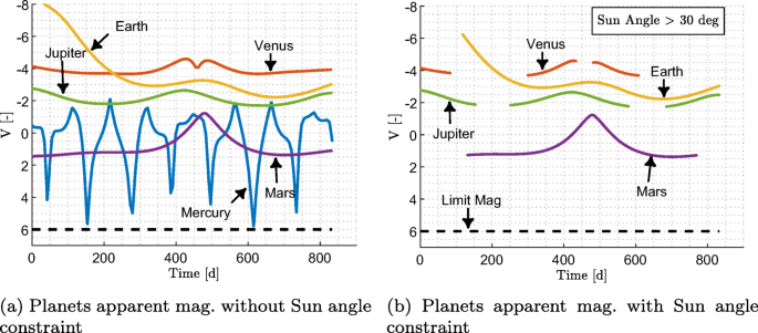
Planets apparent magnitude as seen by M-ARGO towards 2000 SG344: a without Sun angle constraint; b with Sun angle constraint. The horizontal dashed black line is the limit mag. of the sensor
-
(2)
The optimal beacons to be tracked are assessed exploiting the methodology in “Optimal Beacons Selection”. Considering the visible beacons in Fig. 6b, the geometry in terms of γ angles, inertial positions, and LOS directions are the input to the cost function J defined in “Optimal Beacons Selection”. The γ angles between the couples of beacons are shown in Fig. 7a, the figure of merit J for each couple of beacons is shown in Fig. 7b, and the resulting optimal couples of beacons to be tracked per each navigation campaign are shown in Fig. 7c. It is worth reminding that M-ARGO is tracking the optimal beacons in an asynchronous fashion. M-ARGO sticks with the same beacons for each tracking window as a design choice, in order to ease repetitiveness of operations. Moreover, it is remarkable to see that the couple Mars–Jupiter is never optimal for the problem at hand according to the figure of merit J, since Mars and Jupiter are far away with respect to M-ARGO.
Fig. 7 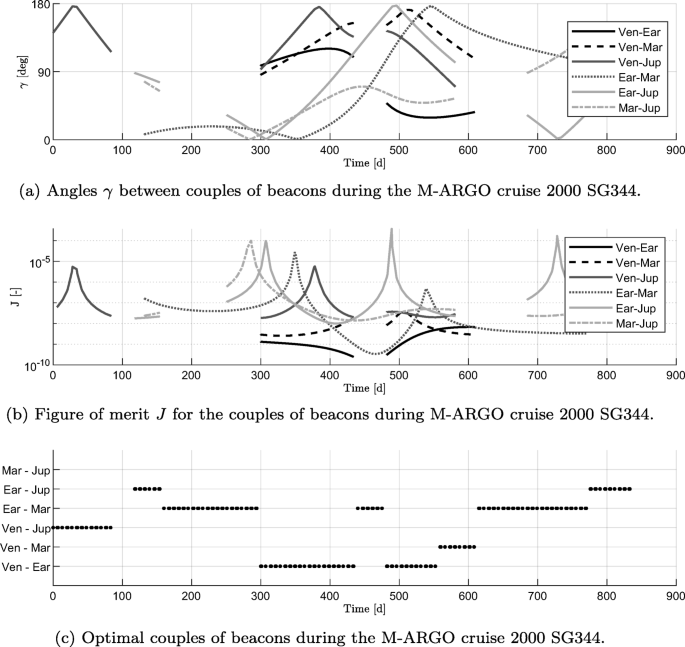
a Angles γ, b index J, and c optimal beacons for M-ARGO towards 2000 SG344
-
(3)
The line-of-sight directions to the visible planets can now be acquired. The accuracy and the settings for the acquisitions are reported in Table 3. Thus, the spacecraft points to a planet for 15 minutes and acquires the LOS with a frequency of 0.0167 Hz (1 per minute). Then, the spacecraft slews to another beacon (slewing time assumed to be 20 minutes) and acquires the LOS to that planet.
-
(4)
The LOS directions are given as input to the Kalman filter formulation to estimate the spacecraft state. The filter outputs in terms of position (δr) and velocity (δv) covariance bounds are shown in Fig. 8a and b.


Position and velocity estimations accuracy exploiting line-of-sight navigation during the M-ARGO cruise to 2000 SG344

Position (δx, δy, δz) and velocity (δvx, δvy, δvz) samples errors (in gray) and 3–σ covariance bounds (in black) for M-ARGO to 2000 SG344. Out of the 1000 filter runs, only 30 have been shown for simplicity
By inspection of Fig. 8a and b, it is remarkable to note that the accuracy in terms of position and velocity reaches values of 103 km and 0.1 m/s in good observation conditions (multiple visible planets approaching 90 deg of γ angles). This is also confirmed by running a Monte Carlo analysis sampling the initial dispersion of the covariance matrix and evaluating the samples covariance with respect to the filter covariance. As it can be seen from Fig. 9, the samples error of each run are always within the 3σ bounds of the filter for the position and velocity components.
The results in terms of beacons observability, relative geometry, and estimation performances for M-ARGO to the selected NEA are encouraging in view of an in-orbit autonomous navigation experiment. Multiple windows to track the optimal beacons along the whole trajectory have been identified to run the experiment and the related performances have been quantified, which are function of the considered performances of a deep-space CubeSat as M-ARGO. All in all, this confirms the availability of multiple windows to run the autonomous navigation experiment during the M-ARGO deep-space cruise and paves the way for further investigation as the M-ARGO project study progresses.
Conclusions
M-ARGO CubeSat mission plans to conduct a deep-space optical navigation experiment in order to reduce operations costs for future missions. The aim is to estimate the spacecraft state through the processing of the line-of-sight directions to a number of visible targets observed by miniaturized onboard optical sensors. The visibility of these navigation beacons is dictated by the relative geometry between the observer and the targets in terms of distances, phase angles, and Sun angles as well as the radiometric performance of the optical sensor used. In this context, an optimal beacons selection criteria has been exploited to assess the optimal couples of beacons to be tracked. Then, the M-ARGO state in terms of position and velocity covariance bounds has been estimated through an extended Kalman filter which is fed by the line-of-sight directions to the navigation beacons.
In good observation conditions, that is when the γ angles between the beacons approach 90 deg as seen from M-ARGO, the accuracy of the optical navigation method is in the order of 1000 km (3σ bounds) in deep-space considering the performance of miniaturized components onboard the 12U CubeSat M-ARGO. Our method appears promising when combined with onboard guidance calculations in view of an autonomous Guidance, Navigation, and Control system. Future steps in developing the navigation experiment during the M-ARGO project involve hardware-in-the-loop simulations with online generation and processing of images to feed the navigation algorithm.
References
Anderson, K., Pines, D., Sheikh, S.: Validation of pulsar phase tracking for spacecraft navigation. J. Guid. Control Dyn. 38(10), 1885–1897 (2015). https://doi.org/10.2514/1.G000789
Banerdt, W.B., Smrekar, S.E., Banfield, D., et al.: Initial results from the InSight mission on Mars. Nat. Geosci. 133(3), 183–189 (2020). https://doi.org/10.1038/s41561-020-0544-y
Borissov, S., Mortari, D.: Centroiding and Sizing Optimization of Ellipsoid Image Processing Using Nonlinear Least-Squares. In: AAS/AIAA Astrodynamics Specialist Conference, Snowbird, UT, pp. 1–14 (2018)
Broschart, S.B., Bradley, N., Bhaskaran, S.: Kinematic approximation of position accuracy achieved using optical observations of distant asteroids. J. Spacecr. Rocket. 56(5), 1383–1392 (2019). https://doi.org/10.2514/1.A34354
Cheng, Y., Crassidis, J.L., Markley, F.L.: Attitude estimation for large field-of-view sensors. J. Astronaut. Sci. 54(3-4), 433–448 (2006). https://doi.org/10.1007/BF03256499
Christian, J.A.: Optical navigation using iterative horizon reprojection. J. Guid. Control Dyn. 39(5), 1092–1103 (2016). https://doi.org/10.2514/1.G001569
Christian, J.A.: Accurate planetary limb localization for image-based spacecraft navigation. J. Spacecr. Rocket. 54(3), 708–730 (2017). https://doi.org/10.2514/1.A33692
Christian, J.A., Crassidis, J.L.: Star identification and attitude determination with projective cameras. IEEE Access 9, 25,768–25,794 (2021). https://doi.org/10.1109/ACCESS.2021.3054836
Christian, J.A., Robinson, S.B.: Noniterative Horizon-Based optical navigation by cholesky factorization. J. Guid. Control Dyn. 39(12), 2757–2765 (2016). https://doi.org/10.2514/1.G000539
Dei Tos, D.A., Baresi, N.: Genetic Optimization for the Orbit Maintenance of Libration Point Orbits with Applications to EQUULEUS and LUMIO. In: AIAA Scitech 2020 Forum, Orlando, pp. 1–18. https://doi.org/10.2514/6.2020-0466 (2020)
Dei Tos, D.A., Rasotto, M., Renk, F., Topputo, F.: Lisa pathfinder mission extension: a feasibility analysis. Adv. Space Res. 63(12), 3863–3883 (2019). https://doi.org/10.1016/j.asr.2019.02.035
Ferrari, F., Franzese, V., Pugliatti, M., Giordano, C., Topputo, F.: Preliminary mission profile of Hera’s Milani CubeSat. Adv. Space Res., 67. https://doi.org/10.1016/j.asr.2020.12.034 (2021)
Franzese, V., Di Lizia, P., Topputo, F.: Autonomous optical navigation for the Lunar Meteoroid Impacts Observer. J. Guid. Control Dyn. 42(7), 1579–1586 (2019). https://doi.org/10.2514/1.G003999
Franzese, V., Topputo, F.: Optimal beacons selection for Deep-Space optical navigation. J. Astronaut. Sci. 67, 1775–1792 (2020). https://doi.org/10.1007/s40295-020-00242-z
Goldberg, H., Karatekin, Ö., Ritter, B., Herique, A., et al.: The Juventas CubeSat in Support of ESA’S Hera Mission to the Asteroid Didymos. In: Small Satellite Conference, Logan, pp. 1–7 (2019)
Kalman, R.E.: A new approach to linear filtering and prediction problems. J. Basic Eng. 82(1), 35–45 (1960). https://doi.org/10.1115/1.3662552
Kalman, R.E., Bucy, R.S.: New results in linear filtering and prediction theory. J. Basic Eng. 83(1), 95–108 (1961). https://doi.org/10.1115/1.3658902
Karimi, R., Mortari, D.: Interplanetary autonomous navigation using visible planets. J. Guid. Control Dyn. 38(6), 1151–1156 (2015). https://doi.org/10.2514/1.G000575
Kawabata, Y., Kawakatsu, Y.: On-board orbit determination using sun sensor and optical navigation camera for deep-space missions. Trans. Jpn. Soc. Aeronaut. Space Sci. 15, 13–19 (2017). https://doi.org/10.2322/tastj.15.13
Klesh, A., Krajewski, J.: MarCO: Cubesats to Mars in 2016. In: 29Th Annual AIAA/USU Conference on Small Satellites, Logan, pp. 1–7 (2015)
Kobylka, K., Christian, J.: Methods in Triangulation for Image-Based Terrain Relative Navigation. In: AAS/AIAA Space Flight Mechanics Meeting, Charlotte (2021)
Kruzelecky, R.: VMMO Lunar Volatile and Mineralogy Mapping 12U Cubesat. In: 42Nd COSPAR Scientific Assembly, Pasadena (2018)
Lockett, T.R., Castillo-Rogez, J., Johnson, L., Matus, J., et al.: Near-earth Asteroid Scout flight mission. IEEE Aerosp. Electron. Syst. Mag. 35(3), 20–29 (2020). https://doi.org/10.1109/MAES.2019.2958729
Malphrus, B.K., Freeman, A., Staehle, R., et al.: Interplanetary CubeSat missions. Elsevier (2020)
Markley, F.L., Crassidis, J.L.: Fundamentals of spacecraft attitude determination and control, Chap. 5, vol. 33. Springer (2014)
McIntosh, D.M., Baker, J.D., Matus, J.A.: The NASA CubeSat Missions Flying on Artemis-1. In: Small Satellite Conference, pp. 1–11. Utah State University, Logan (2020)
Mereta, A., Izzo, D.: Target selection for a small low-thrust mission to near-Earth asteroids. Astrodynamics 2(3), 249–263 (2018). https://doi.org/10.1007/s42064-018-0024-y
Michel, P., Küppers, M., Carnelli, I.: The Hera Mission: European Component of the ESA-NASA AIDA Mission to a Binary Asteroid. In: COSPAR Scientific Assembly, pp. 1–42, Pasadena (2018)
Mortari, D., Conway, D.: Single-point position estimation in interplanetary trajectories using star trackers. Celest. Mech. Dyn. Astron. 156(1), 1909–1926 (2016). https://doi.org/10.1007/s10569-016-9738-4
Mortari, D., D’Souza, C.N., Zanetti, R.: Image processing of illuminated ellipsoid. J. Spacecr. Rocket., 448–456. https://doi.org/10.2514/1.A33342 (2016)
Oguri, K., Oshima, K., Campagnola, S., Kakihara, K., et al.: EQUULEUS Trajectory design. J. Astronaut. Sci., 1–27. https://doi.org/10.1007/s40295-019-00206-y (2020)
Poghosyan, A., Golkar, A.: Cubesat evolution: Analyzing cubesat capabilities for conducting science missions. Progress Aerosp. Sci. 88, 59–83 (2017). https://doi.org/10.1016/j.paerosci.2016.11.002
Racca, G., Marini, A., Stagnaro, L., Van Dooren, J., Di Napoli, L., Foing, B., Lumb, R., Volp, J., Brinkmann, J., Grünagel, R., et al.: SMART-1 mission description and development status. Planetary Space Sci. 50(14-15), 1323–1337 (2002). https://doi.org/10.1016/S0032-0633(02)00123-X
Riedel, J., Bhaskaran, S., Desai, S., Han, D., Kennedy, B., McElrath, T., Null, G., Ryne, M., Synnott, S., Wang, T., et al.: Using Autonomous Navigation for Interplanetary Missions: The Validation of Deep Space 1 AutoNav. In: International Conference on Low-Cost Planetary Missions, Laurel (2000)
Rufino, G., Accardo, D.: Enhancement of the centroiding algorithm for star tracker measure refinement. Acta Astronautica 53(2), 135–147 (2003). https://doi.org/10.1016/S0094-5765(02)00199-6
Schoolcraft, J., Klesh, A., Werne, T.: MarCO: Interplanetary Mission Development on a CubeSat Scale, pp. 221–231. Springer International Publishing, Space Operations: Contributions from the Global Community. https://doi.org/10.1007/978-3-319-51941-8_10 (2017)
Seidelmann, P.K.: Explanatory supplement to the astronomical almanac. University Science Books (2006)
Sheikh, S.I., Pines, D.J., Ray, P.S., et al.: Spacecraft navigation using X-Ray pulsars. J. Guid. Control Dyn. 29(1), 49–63 (2006). https://doi.org/10.2514/1.13331
Shkolnik, E.L.: On the verge of an astronomy cubesat revolution. Nat. Astron. 2 (5), 374–378 (2018). https://doi.org/10.1038/s41550-018-0438-8
Simon, D.: Optimal state estimation: Kalman, H infinity, and nonlinear approaches, pp. 405. Wiley. Chap. 13 (2006)
Speretta, S., Cervone, A., Sundaramoorthy, P., Noomen, R., Mestry, S., Cipriano, A., Topputo, F., Biggs, J., Di Lizia, P., Massari, M., Mani, K.V., Dei Tos, D.A., Ceccherini, S., Franzese, V., Ivanov, A., Labate, D., Tommasi, L., Jochemsen, A., Gailis, J., Furfaro, R., Reddy, V., Vennekens, J., Walker, R.: LUMIO: An Autonomous CubeSat for Lunar Exploration, chap. 6, pp. 103–134. Springer International Publishing. https://doi.org/10.1007/978-3-030-11536-4_6 (2019)
Tapley, B., Schutz, B., Born, G.H.: Statistical orbit determination, chap. 4. Elsevier (2004)
Topputo, F., Massari, M., Biggs, J., Di Lizia, P., Dei Tos, D., Mani, K., Ceccherini, S., Franzese, V., Cervone, A., Sundaramoorthy, P., et al.: LUMIO: a cubesat at Earth-Moon L2. In: 4S Symposium, pp. 1–15. Sorrento (2018)
Topputo, F., Wang, Y., Giordano, C., Franzese, V., Goldberg, H., Perez-Lissi, F., Walker, R.: Envelop of reachable asteroids by m-ARGO CubeSat. Adv. Space Res., 1–50. https://doi.org/10.1016/j.asr.2021.02.031 (2020)
Vaughan, R., Riedel, J., Davis, R., OWEN JR, W., Synnott, S.: Optical Navigation for the Galileo Gaspra Encounter. In: Astrodynamics Conference. https://doi.org/10.2514/6.1992-4522 (1992)
Walker, R., Binns, D., Bramanti, C., Casasco, M., Concari, P., Izzo, D., Feili, D., Fernandez, P., Fernandez, J.G., Hager, P., et al.: Deep-space CubeSats: thinking inside the box. Astron. Geophys. 59(5), 5–24 (2018). https://doi.org/10.1093/astrogeo/aty237
Acknowledgements
The work performed in this paper has been conducted under ESA Contracts No. 4000123920/18/NL/MH and No. 4000127373/19/NL/AF.
Funding
Open access funding provided by Politecnico di Milano within the CRUI-CARE Agreement.
Author information
Authors and Affiliations
Corresponding author
Ethics declarations
Conflict of Interests
The authors have no conflict of interest to declare.
Additional information
Publisher’s Note
Springer Nature remains neutral with regard to jurisdictional claims in published maps and institutional affiliations.
Rights and permissions
Open Access This article is licensed under a Creative Commons Attribution 4.0 International License, which permits use, sharing, adaptation, distribution and reproduction in any medium or format, as long as you give appropriate credit to the original author(s) and the source, provide a link to the Creative Commons licence, and indicate if changes were made. The images or other third party material in this article are included in the article's Creative Commons licence, unless indicated otherwise in a credit line to the material. If material is not included in the article's Creative Commons licence and your intended use is not permitted by statutory regulation or exceeds the permitted use, you will need to obtain permission directly from the copyright holder. To view a copy of this licence, visit http://creativecommons.org/licenses/by/4.0/.
About this article

Cite this article
Franzese, V., Topputo, F., Ankersen, F. et al. Deep-Space Optical Navigation for M-ARGO Mission. J Astronaut Sci 68, 1034–1055 (2021). https://doi.org/10.1007/s40295-021-00286-9
Accepted:
Published:
Issue Date:
DOI: https://doi.org/10.1007/s40295-021-00286-9