An interactive weighted fuzzy goal programming technique to solve multi-objective reliability optimization problem

Abstract

This paper presents an application of interactive fuzzy goal programming to the nonlinear multi-objective reliability optimization problem considering system reliability and cost of the system as objective functions. As the decision maker always have an intention to produce highly reliable system with minimum cost, therefore, we introduce the interactive method to design a high productivity system here. This method plays an important role to maximize the worst lower bound to obtain the preferred compromise solution which is close to the best upper bound of each objective functions. Until the preferred compromise solution is reached, new lower bounds corresponding to each objective functions will be determined based on the present solution to develop the updated membership functions as well as aspiration levels to resolve the proposed problem. Considering judgmental vagueness of decision maker, here we consider the resources as trapezoidal fuzzy numbers and apply total integral value of fuzzy number to transform into crisp one. To illustrate the methodology and performance of this approach, numerical examples are presented and evaluated by comparing with the other method at the end of this paper.

Introduction

Since 1960, reliability engineering is one of the most important tasks in designing and development of a technical system. The primary goal of reliability engineer is always to find the best route to increase the system reliability. The diversity of system resources, resource constraints, and options for reliability improvement leads to the construction and analysis of several optimization models. The majority of reliability optimization models discussed in the various literatures. For example, Misra (1971) discussed the application of integer programming to solve reliability optimization problems. Later Kuo and Prasad (2000) and Kuo et al. (2001) presented some suitable method for solving reliability optimization models. In recent time, Hao et al. (2017) proposed an efficient and robust algorithm of non-probabilistic reliability-based design optimization (NRBDO). Later an efficient and accurate RBDO framework based on iso-geometric analysis (IGA) for complex engineering problems is established by Hao et al. (2019).

In real life system, due to some uncertainty factors in judgments of decision maker (DM), definitely it is not always possible to get consequential data for the reliability optimization model, as there are some coefficients and parameters which are always imprecise due to the vagueness of nature. In order to handle the vague judgments of DM in multi-objective problems, which may be classified as a non-stochastic imprecise model, fuzzy approach can be used to solve this model. Some researchers have also used fuzzy technique to solve multi-objective reliability optimization problems. At first, Park (1987) applied fuzzy optimization techniques to solve the problem of reliability apportionment for a series system. A multi-objective formulation of reliability allocation problem to maximize system reliability and minimize system cost has been described by Sakawa (1978) using surrogate worth trade methods. In recent time, Grag (2013) applied particle swarm optimization method to solve a fuzzy multi-objective reliability optimization problem. Dancese et al. (2014) studied reliability and cost analysis of a series system model using fuzzy parametric geometric programming. Wang et al. (2017) proposed a novel reliability-based optimization model and method for thermal structure design in fuzzy environment.

There are various kinds of optimization techniques which can be used to solve nonlinear optimization problems. Goal programming (GP) is one of the effective methods among those to solve a particular type of nonlinear programming problem. GP has been widely applied to solve different types of real-world problems which involve multiple objectives. After applying GP, the DM can obtain a satisfactory solution and also can able to analyze the aspiration levels. Dhingra (1992) used GP to solve multi-objective reliability apportionment problem in fuzzy environment. Gen and Ida (1993) also discussed the application of large-scale 0–1 fuzzy goal programming to solve reliability optimization problem. Later, Hwang and Lee (2009) provides an algorithm for nonlinear integer goal programming using branch-and-bound method and its application of this algorithm to demonstrate the solving procedure of reliability problems with single and multiple objectives.

In this paper, we are going to introduce a fuzzy multi-objective mathematical programming problem in which system reliability and cost of the system are to be considered as two objective functions. The goal of the present study is to apply an efficient and modified optimization technique to find preferred compromise solution (Leberling 1981) of the proposed model. This is very rare to use interactive weighted fuzzy goal programming (IWFGP) in reliability optimization model. Hence we choose IFGP technique as the solution procedure of the proposed optimization model to design a high productivity system. Wahed and Lee (2006) presented interactive fuzzy goal programming approach to solve multi-objective transportation model. Sakawa and Matsui (2012) and Sinna and Abo-Elnaga (2014) also used interactive approach to solve multi-objective programming under fuzzy environment.

In other existing method like fuzzy multi-objective goal programming (FMOGP) method (Hwang and Lee 2004; Zangiabadi and Maleki 2007), initially the objective goal and the maximum tolerances for resources should be given. In the real-world situations, it is unrealistic to initially ask the decision maker (DM) to give goal and tolerances without providing any information about them. Therefore, the obtained solution may not be satisfactory for the DM. But interactive method considers a large variety of situations that the DM might meet when solving a nonlinear programming problem. In this paper, the proposed interactive approach focuses on maximizing the worst lower bound to obtain the preferred compromise solution which is close to the best upper bound of each objective functions. Updating both the membership values and the aspiration levels during the solution procedure, it controls the search direction. As a result, preferences of DM achieve the efficient solution. This process continues until the decision maker satisfied with the solution. Hence clearly this method gives a highly reliable system compared to other existing methods.

The paper is organized as follows: In “Mathematical model” section, a reliability model of a LCD display unit is considered and develop a multi-objective problem for evaluation; “Prerequisite mathematics” section defines some basic definitions related to fuzzy set; in “Interactive weighted fuzzy goal programming (IWFGP) method” section, IWFGP method is introduced; “Interactive weighted fuzzy goal programming technique on multi-objective fuzzy reliability optimization problem” section provides IWFGP method for solving the proposed reliability model; in “Numerical example” section, numerical examples are solved and compared with the existing methods. Finally, the conclusions are drawn in “Conclusion” section.

Mathematical model

Let $R_{j}$ be the reliability of the jth component of a system and $R_{S} \left( R \right)$ be the system reliability. Let $C_{S} \left( R \right)$ denotes the cost of the system. Here we consider a complex system which includes a five-stage combination reliability model (Fig. 1).

Fig. 1

Reliability model of a LCD display unit

Reliability model of a LCD display unit

Now we are interested to find out the system reliability of a LCD display unit (Neubeck 2004; Mahapatra and Roy 2010) which consists of several components connected to one another. This complex system mainly consists of five stages $L_{i} ,\;\left( {i = 1,2, \ldots ,5} \right)$ which are in series. Thus the generalized formula for the system reliability of the proposed model is given by

$$R_{S} \left( R \right) = L_{1} \times L_{2} \times L_{3} \times L_{4} \times L_{5} = \mathop \prod \limits_{j = 1}^{5} L_{i}$$

(1)

Here

• L₁: LCD panel with reliability R₁, i.e., L₁ = R₁;

• L₂: A backlighting board containing 10 bulbs with individual bulb reliability R₂ such that the board function with at most one bulb failure, i.e., $L_{2} = R_{2}^{10} + 10R_{2}^{9} \left( {1 - R_{2} } \right);$

• L₃: Two microprocessor boards A and B hooked up in parallel, each of reliability R₃, i.e., $L_{3} = 1 - \left( {1 - R_{3} } \right)^{2}$;

• L₄: Dual power supplies in standby redundancy, each power supply of reliability R₄, i.e., $L_{4} = R_{4} + R_{4} \ln \left( {1/R_{4} } \right);$

• L₅: EMI board with reliability R₅ hooked in series with common input of the power supply A, i.e., L₅ = R₅;

Thus we have the following system reliability

$$R_{S} \left( R \right) = R_{1} \left( {R_{2}^{10} + 10R_{2}^{9} \left( {1 - R_{2} } \right)} \right)\left( { 1 - \left( {1 - R_{3} } \right)^{2} } \right)\left( {R_{4} + R_{4} \ln \left( {1/R_{4} } \right)} \right) R_{5}$$

(2)

Multi-objective reliability optimization model (MOROM)

Here we consider the cost of the proposed complex system as an additional objective function. Therefore, the system reliability and the cost of the system are to be maximized and minimized, respectively subject to system space as target goal. Thus the model becomes

$$\begin{aligned} & {\text{Max}}\;R_{S} \left( R \right) = R_{1} \left( {R_{2}^{10} + 10R_{2}^{9} \left( {1 - R_{2} } \right)} \right)\left( { 1 - \left( {1 - R_{3} } \right)^{2} } \right)\left( {R_{4} + R_{4} \ln \left( {1/R_{4} } \right)} \right)R_{5} \\ & {\text{Min}}\;C_{S} \left( R \right) = \mathop \sum \limits_{j = 1}^{5} c_{j} \left[ {\tan \left( {\frac{\pi }{2}} \right)R_{j} } \right]^{{\alpha_{j} }} \\ & {\text{s}} . {\text{t}} .\;V_{S} \left( R \right) = \mathop \sum \limits_{j = 1}^{5} v_{j} R_{j}^{{a_{j} }} \le V_{ \lim } \\ & 0.5 \le R_{j,{\rm min} } \le R_{j} \le 1,0 \le R_{S} \le 1;\;j = 1,2, \ldots ,5 \\ \end{aligned}$$

(3)

Here $v_{j}$ and $c_{j}$ represent the space and cost of the jth component of the system, respectively. $V_{ \lim }$ is the system space limitation and $R_{{j,{ {\rm min} }}}$ is the lower bound of the reliability of each component j.

Now to simplify the calculation and to convert the above problem to one type maximization problem, we consider

$$C_{S}^{\prime } (R) = - C_{S} (R)$$

Thus model (3) has the following form

$$\begin{aligned} & {\text{Max}}\;R_{S} (R) \\ & {\text{Max}}\;C_{S}^{\prime } (R) \\ \end{aligned}$$

(4)

subject to the same constraints defined in (3)

Multi-objective fuzzy reliability optimization model

In general the coefficients of cost parameters, resources of constraints are not always be specified by relevant precise data and has always been imprecise and vague in nature. This type of imprecise data is not always well represented by random variable selected from a probability distribution. But fuzzy number may represent these data. Here we consider space goal $V_{ \lim }$ as trapezoidal fuzzy number which can be expressed as $\tilde{V}_{ \lim } = (V_{1L} ,V_{2L} ,V_{3L} ,V_{4L} )$). Thus the above problem (4) reduces to the following fuzzy problem as

$$\begin{aligned} & {\text{Max}}\;R_{S} (R) = R_{1} \left( {R_{2}^{10} + 10R_{2}^{9} \left( {1 - R_{2} } \right)} \right)\left( { 1 - \left( {1 - R_{3} } \right)^{2} } \right)\left( {R_{4} + R_{4} \ln \left( {1/R_{4} } \right)} \right)R_{5} \\ & {\text{Max}}\;C_{S}^{{\prime }} (R) = - \mathop \sum \limits_{j = 1}^{5} c_{j} \left[ {\tan \left( {\frac{\pi }{2}} \right)R_{j} } \right]^{{\alpha_{j} }} \\ & {\text{s}} . {\text{t}} .\;V_{S} (R) = \mathop \sum \limits_{j = 1}^{5} v_{j} R_{j}^{{a_{j} }} \le \tilde{V}_{ \lim } \\ & 0.5 \le R_{j,{\rm min} } \le R_{j} \le 1,\;0 \le R_{S} \le 1;\;j = 1,2, \ldots ,5 \\ \end{aligned}$$

(5)

Prerequisite mathematics

Definition 3.1

A $fuzzy\;set\;\tilde{A}$ in X is a set of ordered pairs (Zadeh 1965 first introduced the fuzzy set theory):

$$\tilde{A} = \left\{ {\left( {x,\mu_{{\tilde{A}}} (x)} \right)| x \in X} \right\},$$

where X is a collection of objects denoted generically by x and $\mu_{{\tilde{A}}} \left( x \right):X \to \left[ {0,1} \right]$ is called the membership function or grade of membership of x in $\tilde{A}$.

Definition 3.2

Chen (Chen 1985) represents a generalized trapezoidal fuzzy number (GTrFN) $\tilde{A}$ as $\tilde{A} = (a,b,c,d;w)$, where $0 < w \le 1,$ and a, b, c, and d are real numbers. The generalized fuzzy number $\tilde{A}$ is a fuzzy subset of real line R, whose membership function $\mu_{{\tilde{A}}} (x):R \to \left[ {0,w} \right]$ is defined as

$$\mu_{{\tilde{A}}}^{w} (x) = \left\{ {\begin{array}{*{20}l} {\mu_{{L\tilde{A}}}^{w} (x) = w \frac{x - a}{b - a} ,} \hfill & {a \le x \le b;} \hfill \\ {w,} \hfill & {b \le x \le c;} \hfill \\ {\mu_{{R\tilde{A}}}^{w} (x) = w \frac{x - d}{c - d}, } \hfill & {c \le x \le d;} \hfill \\ {0,} \hfill & {\text{otherwise}} \hfill \\ \end{array} } \right.$$

(6)

Note: $\tilde{A}$ is a normalized fuzzy number when w = 1, and it is non-normalized for w ≠ 1 (Fig. 2).

Fig. 2

Generalized trapezoidal fuzzy number

Here $\mu_{{L\tilde{A}}}^{w }$ and $\mu_{{R\tilde{A}}}^{w}$ are the left and right membership functions of $\tilde{A}$ respectively.

And the inverse functions $h_{{L\tilde{A}}}^{w} :\left[ {0,w} \right] \to \left[ {a,b} \right]$ and $h_{{R\tilde{A}}}^{w} :\left[ {0,w} \right] \to \left[ {{\text{c}},{\text{d}}} \right]$ are defined as

$$h_{{L\tilde{A}}}^{w} (y) = a + \frac{{\left( {b - a} \right)}}{w}y;$$

(7)

$$h_{{R\tilde{A}}}^{w} (y) = d + \frac{{\left( {c - d} \right)}}{w}y;\;y \in \left[ {0,w} \right].$$

Now according to integral value method of Liou’s (Liou and Wang 1992) we have, for a non-normal fuzzy number $\tilde{A}$, the corresponding membership function $f_{{\tilde{A}}} (x)$ can be normalized by dividing the maximal value of $f_{{\tilde{A}}} (x)$, i.e., w and let $\bar{\tilde{A}}$ and $\bar{f}_{{\tilde{A}}}$ are normalized fuzzy number and the corresponding membership function.

Let $k \in \left[ {0,1} \right]$ be the index of optimism which represent the degree of optimism of a decision maker (DM). then the total k-integral value is defined as

$$I_{k}^{w} (\tilde{A}) = \left[ {kI_{R}^{w} (\tilde{A}) + \left( {1 - k} \right)I_{L}^{w} (\tilde{A})} \right]$$

where $I_{wR} (\tilde{A})$ and $I_{wL} (\tilde{A})$ represent the right and left integral values of $\tilde{A}$, respectively. Now, when $\tilde{A}$ being ranked, using the result discussed in Liou and Wang (1992), we have

$$\begin{aligned} I_{L}^{w} (\tilde{A}) & = \int_{0}^{1} {h_{{L\tilde{A}}}^{w} } \left( {wy} \right){\text{d}}y = \frac{1}{2}\left( {a + b} \right) \\ {\text{and}}\;I_{R}^{w} (\tilde{A}) & = \int_{0}^{1} {h_{{R\tilde{A}}}^{w} } \left( {wy} \right) {\text{d}}y = \frac{1}{2}\left( {c + d} \right) \\ \end{aligned}$$

Thus, $I_{k}^{w} (\tilde{A}) = \frac{1}{2}\left[ {k\left( {c + d} \right) + \left( {1 - k} \right)\left( {a + b} \right)} \right]$ which does not depend on the value of w, i.e., whether $\tilde{A}$ is normal or not. A larger value of k indicates the higher degree of optimism. Now for k = 0, the total k-integral value is $I_{0}^{w} (\tilde{A}) = \frac{1}{2}\left( {a + b} \right) = I_{w}^{L} (\tilde{A})$, represents a pessimistic viewpoint of a DM and for optimistic DM’s viewpoint, i.e., for $k = 1,\;I_{1}^{w} (\tilde{A}) = \frac{1}{2}\left( {c + d} \right) = I_{w}^{R} (\tilde{A})$. When k = 0.5, the total k-integral value $I_{0.5}^{w} (\tilde{A}) = \frac{1}{2}\left[ {I_{w}^{R} (\tilde{A}) + I_{w}^{L} (\tilde{A})} \right]$ reflects a moderately optimistic DM’s viewpoint.

Interactive weighted fuzzy goal programming (IWFGP) method

The interactive method is an efficient and modified optimization technique and gives a highly reliable system than other existing methods. At the time of solving a nonlinear programming problem, interactive method considers a large variety of situations that the decision maker (DM) might meet. In this method DM can modify the original model continuously to obtain a satisfactory solution until the decision maker will be satisfied with the obtained result at each stage.

Here we are presenting a solution procedure to solve multi-objective reliability optimization problem (MOROP) by interactive weighted fuzzy goal programming technique and the following steps are used

Step 1 Construct a fuzzy multi-objective nonlinear programming problem considering k objective functions as

$$\begin{aligned} & {\text{Maximize}}\,(f_{1} (x),f_{2} (x), \ldots , f_{k} (x)) \\ & {\text{Subject}}\;{\text{to}},\quad g_{i} (x) \le \tilde{b}_{i} ,\quad i = 1,2, \ldots ,m;\quad x \ge 0; \\ \end{aligned}$$

(8)

Step 2 Solve the fuzzy multi-objective nonlinear programming problem taking only one objective function at a time and avoid the others, so that we can get the ideal solutions. If all the solutions are the same, select one of them as an optimal compromise solution and go to step 10. Otherwise go to step 3.

Step 3 With the values of all objective functions evaluated at these ideal solutions, the payoff matrix can be formulated as follows (Table 1)

Table 1 Payoff matrix of the solution of (8)

Step 4 Determine the best upper bound and the worst lower bound for constructing the membership function as follows

$$\begin{aligned} U_{r} = \hbox{max} \;\left\{ {f_{r} (x^{1} ),f_{r} \left( {x^{2} } \right), \ldots ,f_{r} \left( {x^{k} } \right)} \right\}\quad \forall r = 1,2, \ldots ,k \hfill \\ {\text{and}}\;L_{r} = \hbox{min} \;\left\{ {f_{r} (x^{1} ),f_{r} \left( {x^{2} } \right), \ldots ,f_{r} \left( {x^{k} } \right)} \right\}\quad \forall r = 1,2, \ldots ,k \hfill \\ \end{aligned}$$

So, $L_{r} \le f_{r} \left( x \right) \le U_{r}$

Here L_r and U_r are, respectively, lower and upper bounds of the rth objective function $f_{r} (x),\quad \forall r = 1,2, \ldots ,k.$

Step 5 Construct the membership functions of each objective functions as follows

$$\mu_{r}^{{w_{r} }} (f_{r} (x)) = \left\{ {\begin{array}{*{20}l} 0 \hfill & {{\text{if}}\;\;f_{r} (x) < L_{r} ;} \hfill \\ {w_{r} \frac{{f_{r} \left( x \right) - L_{r} }}{{U_{r} - L_{r} }}} \hfill & {{\text{if}}\;\;L_{r} \le f_{r} (x) \le U_{r} ;\quad \forall r = 1,2, \ldots ,k.} \hfill \\ {w_{r} } \hfill & {{\text{if}}\;U_{r} < f_{r} (x);} \hfill \\ \end{array} } \right.$$

(9)

and

$$\mu_{r} \left( {g_{i} (x)} \right) = \left\{ {\begin{array}{*{20}l} 0 \hfill & {{\text{if}}\;\;b_{i} + p_{i} < g_{i} (x);} \hfill \\ {1 - \frac{{g_{i} (x) - b_{i} }}{{p_{i} }}} \hfill & {{\text{if}}\;\;b_{i } \le g_{i} (x) \le b_{i} + p_{i} ;\quad \forall i = 1,2, \ldots ,m.} \hfill \\ 1 \hfill & {{\text{if}}\;\;g_{i} (x) < b_{i} ;} \hfill \\ \end{array} } \right.$$

(10)

U_r is the best upper bound and L_r is the worst lower bound of the rth objective functions, respectively.

Step 6 Now based on the max–min operator introduced by Bellman and Zadeh (1970), the following decision making is defined as

$${\text{fuzzy}}\;{\text{decisions (}}D )= {\text{fuzzy}}\;{\text{objective}}\;{\text{goals}}\;(G) \cap {\text{fuzzy}}\;{\text{constraints (}}C )$$

Thus, the membership function is characterized by

$$\mu_{D} (x) = \hbox{min} \left( {\mu_{G} (x) , \mu_{C} (x)} \right)$$

Introducing the variable λ, where

$$\begin{aligned} \lambda & = { \hbox{min} }\left[ {\mu_{1}^{{w_{1} }} \left( {f_{1} (x)} \right), \ldots ,\mu_{k}^{{w_{k} }} \left( {f_{k} (x)} \right)} \right]\varvec{ } \\ & = { \hbox{min} }\left[ {\mu_{1}^{w} \left( {f_{1} (x)} \right), \ldots ,\mu_{k}^{w} \left( {f_{k} (x)} \right)\varvec{ }} \right] \\ & = { \hbox{min} }\left[ {w\mu_{1} \left( {f_{1} \left( x \right)} \right), \ldots ,w\mu_{k} \left( {f_{k} (x)} \right)} \right]\quad {\text{Where}},\;w = {\text{min(}}w_{1} ,w_{2} , \ldots ,w_{k} )\\ & = { \hbox{min} }_{r} (w_{r} ),\;{\text{for}}\,r = 1,2, \ldots ,k. \\ \end{aligned}$$

Step 7 Obtain a preferred solution by solving the following problem:

$$\begin{aligned} & \quad \quad \quad \quad \quad \quad {\text{Maximize}}\;\lambda \\ & {\text{Subject}}\;{\text{to}},\quad w\mu_{r} (f_{r} (x)) \ge \lambda ;\quad \forall r = 1,2, \ldots ,k; \\ & \quad \quad \quad \quad \quad \;\;\;\mu_{i} \left( {g_{i} (x)} \right) \ge \lambda ;\quad \forall i = 1,2, \ldots ,m; \\ & \quad \quad \quad \quad \quad \;\;\lambda \in \left[ {0,w} \right]\;{\text{and}}\; x \ge 0,\;w \in \left( {0,1} \right] \\ \end{aligned}$$

(11)

Now using positive weights W_r (r = 1,2, …, k) for the objectives f_r(x), we have

$$\begin{aligned} & \quad \quad \quad \quad \quad \quad {\text{Maximize}}\;\lambda \\ & {\text{Subject}}\;{\text{to}},\quad W_{r} \;w\mu_{r} (f_{r} (x)) \ge \lambda ;\quad \forall r = 1,2, \ldots , k; \\ & \quad \quad \quad \quad \quad \;\;\;\mu_{i} \left( {g_{i} (x)} \right) \ge \lambda ;\quad \forall i = 1,2, \ldots ,m; \\ & \quad \quad \quad \quad \quad \;\;\lambda \in \left[ {0,w} \right]\;{\text{and}}\; x \ge 0,\;w \in \left( {0,1} \right],\;\mathop \sum \limits_{r = 1}^{k} W_{r} = 1. \\ \end{aligned}$$

(12)

Here positive weights W_r (r = 1, 2, …, k) reflect the decision maker’s preferences regarding the relative importance of each objective goal.

Step 8 Now to convert the problem to a nonlinear goal programming problem, positive and negative deviational variables $\delta_{k}^{ + }$ and $\delta_{k}^{ - }$ are introduced, respectively. Thus the goal programming problem is as follows

$$\begin{aligned} & {\text{Maximize}}\;\lambda \\ & {\text{Subject}}\;{\text{to}},\quad W_{r} \;w\mu_{r} (f_{r} (x)) \ge \lambda ;\quad \forall r = 1,2, \ldots , k; \\ & \quad \quad \quad \quad \quad \;\;\;\mu_{i} \left( {g_{i} (x)} \right) \ge \lambda ;\quad \forall i = 1,2, \ldots ,m; \\ & \quad \quad \quad \quad \quad \;\;\;f_{r} (x) - \delta_{k}^{ + } + \delta_{k}^{ - } = G_{r} \\ & \quad \quad \quad \quad \quad \;\;\;x,\delta_{k}^{ + } ,\delta_{k}^{ - } \ge 0,\quad r = 1,2, \ldots , k; \\ & \quad \quad \quad \quad \quad \;\;\lambda \in \left[ {0,w} \right]\;{\text{and}}\; w \in \left( {0,1} \right],\;\mathop \sum \limits_{r = 1}^{k} W_{r} = 1. \\ \end{aligned}$$

(13)

where G_r is the aspiration level of rth objective function.

Step 9 Evaluate each objective function corresponding to the solution vector $R^{*}$ and find $f_{1}^{*} ,f_{2}^{*} , \ldots , f_{k}^{*} .$

$$\begin{array}{*{20}l} {\text{Now,}} \hfill & {{\text{if}}({\text{i}})} \hfill & {f_{k}^{*} > L_{k} ,\;{\text{then}}\;L_{k} \;{\text{is}}\;{\text{replaced}}\;{\text{by}}\;f_{k}^{*} .} \hfill \\ {} \hfill & {{\text{if}}({\text{ii}})} \hfill & {f_{k}^{*} > L_{k} ,\,{\text{then}}\;{\text{keep}}\;{\text{these}}\;{\text{aspiration}}\,{\text{level}}\;{\text{same}}.} \hfill \\ {\text{and}} \hfill & {{\text{if}}({\text{iii}})} \hfill & {f_{k}^{*} = U_{k} ,\;{\text{then}}\;{\text{replace}}\;L_{k} \;{\text{by}}\;U_{k} \;{\text{and}}\;{\text{keep}}\;{\text{them}}\;{\text{until}}\;{\text{the}}\;{\text{solution}}\;{\text{procedure}}\;{\text{is}}\;{\text{terminated}}.} \hfill \\ \end{array}$$

If the preferred solution obtained from (13) is satisfactory for the decision maker (DM), then the process is successfully concluded and go to step 10. Otherwise go to step 5 and repeat the process.

Step 10 Stop.

There are some restrictions on modifying the membership functions of objectives and fuzzy constraints (See “Appendix”).

Interactive weighted fuzzy goal programming technique on multi-objective fuzzy reliability optimization problem

To solve the above defined model (5), using “Interactive weighted fuzzy goal programming (IWFGP) method” section payoff matrix is formulated as follows:

	$R_{S} \left( R \right)$	$C_{S}^{{\prime }} \left( R \right)$
$R^{1}$	$R_{S}^{*} \left( {R^{1} } \right)$	$C_{S}^{{\prime }} \left( {R^{1} } \right)$
$R^{2}$	$R_{S} (R^{2} )$)	$C_{S}^{{{\prime }*}} \left( {R^{2} } \right)$

Now the best upper bound and worst lower bound are identified, which are given by U₁, U₂, and $L_{1} ,L_{2}$, respectively.

Where $L_{1} \le R_{S} \left( R \right) \le U_{1} ;\quad L_{2} \le C_{S}^{{\prime }} \left( R \right) \le U_{2}$

$$\begin{aligned} & U_{1} = \hbox{max} \left\{ {R_{S} (R^{1} ),\;R_{S} (R^{2} )} \right\};\quad U_{2} = \hbox{max} \left\{ {C_{S}^{\prime } (R^{1} ),\;C_{S}^{\prime } (R^{2} )} \right\} \\ & L_{1} = \hbox{min} \left\{ {R_{S} (R^{1} ),\;R_{S} (R^{2} )} \right\};\quad L_{2} = \hbox{min} \left\{ {C_{S}^{\prime } (R^{1} ),\;C_{S}^{\prime } (R^{2} )} \right\} \\ \end{aligned}$$

Now the linear membership functions for the objectives $R_{S} (R)$, $C_{S} \left( R \right)$ and constraint $V_{S} \left( R \right)$ are defined as follows:

$$\mu_{{R_{S} }}^{{w_{1} }} \left( {R_{S} (R)} \right) = \left\{ {\begin{array}{*{20}l} 0 \hfill & {{\text{if}}\;R_{S} (R) < L_{1} ;} \hfill \\ {w_{1} \left( {\frac{{R_{S} (R) - L_{1} }}{{U_{1} - L_{1} }}} \right)} \hfill & {{\text{if}}\;L_{1} \le R_{S} (R) \le U_{1} ;} \hfill \\ {w_{1} } \hfill & {{\text{if}}\;U_{1} < R_{S} (R);} \hfill \\ \end{array} } \right.$$

(14)

$$\mu_{{C_{S}^{\prime } }}^{{w_{2} }} \left( {C_{S}^{\prime } (R)} \right) = \left\{ {\begin{array}{*{20}l} 0 \hfill & {{\text{if}}\;\;C_{S}^{\prime } (R) < L_{2} ;} \hfill \\ {w_{2} \left( {\frac{{C_{S}^{\prime } (R) - L_{2} }}{{U_{2} - L_{2} }}} \right)} \hfill & {{\text{if}}\;\;L_{2} \le C_{S}^{\prime } (R) \le U_{2} ;} \hfill \\ {w_{2} } \hfill & {{\text{if}}\;\;U_{2} < C_{S}^{\prime } (R);} \hfill \\ \end{array} } \right.$$

(15)

and

$$f_{{V_{S} }} \left( {V_{S} (R)} \right) = \left\{ {\begin{array}{*{20}l} 0 \hfill & {{\text{if}}\;\;V_{ \lim } + d_{{V_{S} }} < V_{S} (R);} \hfill \\ {1 - \left( {\frac{{V_{S} (R) - V_{ \lim } }}{{d_{{V_{S} }} }}} \right)} \hfill & {{\text{if}}\;\;V_{ \lim } \le V_{S} (R) \le V_{ \lim } + d_{{V_{S} }} ;} \hfill \\ 1 \hfill & {{\text{if}}\;\;V_{S} (R) < V_{ \lim } ;} \hfill \\ \end{array} } \right.$$

(16)

After electing the membership functions, the crisp model is formulated as follows

$$\begin{aligned} & \quad \quad \quad \quad \quad {\text{Maximize}}\;\lambda \\ & {\text{Subject}}\;{\text{to}}, \\ & \quad \quad \quad \quad \quad \quad \quad W_{1} w\left( {\frac{{R_{S} (R) - L_{1} }}{{U_{1} - L_{1} }}} \right) \ge \lambda ; \\ & \quad \quad \quad \quad \quad \quad \quad W_{2} w\left( {\frac{{C_{S}^{\prime } (R) - L_{2} }}{{U_{2} - L_{2} }}} \right) \ge \lambda ; \\ & d_{{V_{S} }} \left( {1 - \lambda } \right) - \mathop \sum \limits_{j = 1}^{5} v_{j} R_{j}^{{a_{j} }} - \left( {I(V_{ \lim } )} \right) \ge 0; \\ & 0.5 \le R_{{j,{ {\rm min} }}} \le R_{j} \le 1,0 \le R_{S} \le 1;\lambda \in \left[ {0,w} \right]\;{\text{and}}\;w \in \left( {0,1} \right],\mathop \sum \limits_{r = 1}^{2} W_{r} = 1. \\ \end{aligned}$$

(17)

Here $I(V_{ \lim } )$ denote the integral value of the space limitation of the system (Fig. 3).

Fig. 3

The whole procedure of the proposed model

Now from the above problem, we have the goal programming problem is as follows

$$\begin{aligned} & \quad \quad \quad \quad \quad {\text{Maximize}}\;\lambda \\ & {\text{Subject}}\;{\text{to}}, \\ & \quad \quad \quad \quad \quad \quad \quad W_{1} w\left( {\frac{{R_{S} (R) - L_{1} }}{{U_{1} - L_{1} }}} \right) \ge \lambda ; \\ & \quad \quad \quad \quad \quad \quad \quad W_{2} w\left( {\frac{{C_{S}^{\prime } (R) - L_{2} }}{{U_{2} - L_{2} }}} \right) \ge \lambda ; \\ & d_{{V_{S} }} \left( {1 - \lambda } \right) - \mathop \sum \limits_{j = 1}^{5} v_{j} R_{j}^{{a_{j} }} - \left( {I(V_{ \lim } )} \right) \ge 0; \\ & {\text{R}}_{\text{S}} ({\text{R}}) - \delta_{{{\text{R}}_{\text{S}} }}^{ + } + \delta_{{{\text{R}}_{\text{S}} }}^{ - } = G_{{{\text{R}}_{\text{S}} }} ; \\ & {\text{C}}_{\text{S}}^{{\prime }} ({\text{R}}) - \delta_{{{\text{C}}_{{{\text{S}}^{{\prime }} }} }}^{ + } + \delta_{{{\text{C}}_{{{\text{S}}^{{\prime }} }} }}^{ - } = G_{{{\text{C}}_{\text{S}} }} ; \\ & 0.5 \le R_{{j,{ {\rm min} }}} \le R_{j} \le 1,\;0 \le R_{S} \le 1;\lambda \in \left[ {0,w} \right]\;{\text{and}}\;w \in \left( {0,1} \right],\mathop \sum \limits_{r = 1}^{2} W_{r} = 1. \\ & \delta_{{{\text{R}}_{\text{S}} }}^{ + } ,\delta_{{{\text{R}}_{\text{S}} }}^{ - } ,\delta_{{{\text{C}}_{\text{S}}^{{\prime }} }}^{ + } ,\delta_{{{\text{C}}_{\text{S}}^{{\prime }} }}^{ - } \ge 0; \\ \end{aligned}$$

(18)

Numerical example

Now a five-stage combination reliability model of a complex system is considered for numerical exposure. The problem becomes as follows (Table 2):

$$\begin{aligned} & {\text{Max}}\;R_{S} (R) = R_{1} \left( {R_{2}^{10} + 10R_{2}^{9} \left( {1 - R_{2} } \right)} \right)\left( { 1 - \left( {1 - R_{3} } \right)^{2} } \right)\left( {R_{4} + R_{4} { \ln }\left( {1/R_{4} } \right)} \right)R_{5} \\ & {\text{Min}}\;C_{\text{S}} \left( R \right) = \mathop \sum \limits_{j = 1}^{5} c_{j} \left[ {\tan \left( {\frac{\pi }{2}} \right)R_{j} } \right]^{{\alpha_{j} }} \\ & {\text{s}} . {\text{t}} .\;V_{S} \left( R \right) = \mathop \sum \limits_{j = 1}^{5} v_{j} R_{j}^{{a_{j} }} \le V_{ \lim } \\ & 0.5 \le R_{j,{\rm min} } \le R_{j} \le 1,0 \le R_{S} \le 1;\;j = 1,2, \ldots ,5 \\ \end{aligned}$$

(19)

Table 2 The input data for the MOROM (19)

Here we consider the resource V_lim as triangular fuzzy number and taking the fuzzy input data as $\tilde{V}_{ \lim } = \left( {23.5,24.5,26.5,27.5} \right)$ for k = 0.5 and for each objective function solution vectors is given by (Table 3)

$$\begin{aligned} & R^{1} = \left( {0.999999,0.996198,0.872375,0.815615,0.999999} \right)\;{\text{and}} \\ & R^{2} = \left( {0.500000,0.500000,0.500000,0.500000,0.500000 } \right) \\ \end{aligned}$$

Table 3 Payoff matrix of the solution of (19)

Now the upper and lower bound are given by (Table 4) $U_{1} = 0.9652396,\;U_{2} = - 156.059;$$L_{1} = 0.0017051,\;L_{2} = - 5442.103;$ and can be written as $0.0017051 \le R_{S} \left( R \right) \le 0.9652396$ and $- 5442.103 \le C_{S}^{\prime } \left( R \right) \le - 156.059;$

Table 4 First modified compromise solutions of (19)

The membership functions of objectives and constraints are formulated and solving the goal programming problem (18) using LINGO package we have

The new upper and lower bound are $0.206754 \le R_{S} \left( R \right) \le 0.9652396$ and $- 3964.032 \le C_{S}^{\prime } \left( R \right) \le - 156.059$. Thus the new aspiration levels of the two objective functions are 0.206754 and − 3964.032, respectively. Assume that the decision maker (DM) is not satisfied with this solution and needs more satisfactory solution and thus according to discussion on modification of membership function in “Interactive weighted fuzzy goal programming (IWFGP) method” section, DM modified and resolved the model and will get the following compromise solution (Table 5):

Table 5 Second modified compromise solution of (19)

Now if the DM considers this solution as preferred compromise solution, then the procedure is terminated, but if not, then the process will continue until DM will accept the result. Thus we have the following set of compromise solutions $\left( {R_{S} \left( R \right),C_{S}^{\prime } \left( R \right)} \right)$ as: (0.0017051, − 5442.103), (0.206754, − 3964.032), (0.605869, − 2469.679), (0.820822, − 2017.214), (0.869041, − 1184.530), (0.959681, − 619.152), respectively.

Thus the proposed interactive weighted fuzzy goal programming (IWFGP) method gives the preferred compromise solution as $R_{S} \left( R \right) = 0.959681$ and $C_{S}^{\prime } \left( R \right) = - 619.152.$

According to Wahed and Lee (2006), to determine the degree of closeness of the result obtained by IWFGP approach results to the ideal solution, we define the following distance functions (Steuer 1986) as

$$D_{\rho } \left( {\beta ,K} \right) = \left[ {\mathop \sum \limits_{r = 1}^{K} \beta_{r}^{\rho } \left( {1 - d_{r} } \right)^{\rho } } \right]^{{{\raise0.7ex\hbox{$1$} \!\mathord{\left/ {\vphantom {1 \rho }}\right.\kern-0pt} \!\lower0.7ex\hbox{$\rho $}}}}$$

(20)

where $\rho$ is a distance parameter and $1 \le \rho \le \infty$. d_r represents the degree of closeness of the preferred compromise solution to the optimal solution vector of the rth objective function

$${\text{i}} . {\text{e}} .\quad d_{r} = \frac{{{\text{the}}\;{\text{optimal}}\;{\text{solution }}\;{\text{of}}\;{\text{rth}}\;{\text{objective}}\;{\text{function}}}}{{{\text{the}}\;{\text{preferred}}\;{\text{compromise}}\;{\text{solution}}\;{\text{of}}\;{\text{rth}}\;{\text{objective}}\;{\text{function}}}}$$

$\beta = \left( {\beta_{1} ,\beta_{2} } \right)$ is the vector of objectives aspiration levels and $\sum\nolimits_{L = 1}^{2} {\beta_{L} } = 1$. Now for $\rho = 1,2\;and\;\infty$ we have the distance functions as follows:

• (i) $D_{1} \left( {\beta ,K} \right) = 1 - \mathop \sum \limits_{r = 1}^{K} \beta_{r} d_{r}$

• (ii) $D_{2} \left( {\beta ,K} \right) = \left[ {\mathop \sum \limits_{r = 1}^{K} \beta_{r}^{2} \left( {1 - d_{r} } \right)^{2} } \right]^{{{\raise0.7ex\hbox{$1$} \!\mathord{\left/ {\vphantom {1 2}}\right.\kern-0pt} \!\lower0.7ex\hbox{$2$}}}}$

• (iii)
  $$D_{\infty } \left( {\beta ,K} \right) = \max_{r} \left\{ {\beta_{r} \left( {1 - d_{r} } \right)} \right\}$$

  (21)

In the given numerical example we take $\beta_{1} = \beta_{2} = 0.5,$ (i.e., the objectives are equally important) and compare the solution of (19) with different approaches.

From Table 6, it is clear that the suggested approach gave a better preferred compromise solution and also in $D_{1} ,\;D_{2} \;{\text{and}}\;D_{\infty }$ compared to the solution obtained by intuitionistic fuzzy approach in Mahapatra and Roy (2010) and FMOGP method.

Table 6 Comparison of solutions with different approaches (for W₁ = W₂ = 0.5 and w = 0.9)

Conclusion

Here we introduced interactive fuzzy-weighted goal programming method to find the preferred compromise solution of the proposed multi-objective reliability optimization model. Also here we consider the resources as trapezoidal fuzzy number and used the total integral value of fuzzy number to convert into crisp number. The main advantage of interactive approaches is that the DM controls the search direction during the solution procedure and as a result, the DM’s preferences achieve efficient solutions. In this paper the proposed approach focuses on maximizing the worst lower bound to obtain the preferred compromise solution which is close to the best upper bound of each objective functions. Updating both the membership values and the aspiration levels during the solution procedure, it controls the search direction. Thus the proposed method is an efficient and modified optimization technique and gives a highly reliable system than the other existing methods. An illustrative numerical example was provided by comparing the result obtained in the interactive method with the other methods to demonstrate the efficiency of the proposed method.

Appendix

In the proposed interactive method there are some restrictions on modifying the membership functions of objectives and fuzzy constraints. Only the following variations are acceptable for modification:

• 1. Increase in L_r: Increase in L_r leads to the rise of requirement on the pth objective. All feasible solutions x with $f_{r} (x) < L_{r} \left( {\text{new}} \right)$ are eliminated from the new feasible solution set. Now, we should increase as few requirements as possible in each iteration to avoid the possibility of getting into empty feasible solutions set because of excess increases of L_r. We must be very careful to modify U_r when the decision maker insists on changing U_r, because reduction of the upper bound U_r can lead to an inefficient solution.

• 2. For the constrains, ≤ , ≥ , = , the decrease of p_i is an acceptable modification which can guarantee an efficient solution in the recalculated compromise solution step. The consequence of an increase of p_i with ≤ , ≥ , = constraints might be, for example, that the feasible solution set increases and new possible solutions are included in the investigation (Fig. 4).

  Fig. 4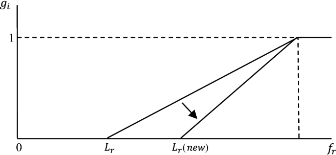

  

  The effects of changing L_r

References

Bellman RE, Zadeh LA (1970) Decision making in a fuzzy environment. Manage Sci 17(4):B141–B164
Chen SH (1985) Ranking fuzzy numbers with maximizing set and minimizing set. Fuzzy Sets Syst 17:113–129
Dancese M, Abbas F, Ghamry E (2014) Reliability and cost analysis of a series system model using fuzzy parametric geometric programming. Int J Innov Sci Eng Technol 1(8):18–23
Dhingra AK (1992) Optimal apportionment of reliability and redundancy in series system under multiple objectives. IEEE Trans Reliab 41:576–582
Gen M, Ida K (1993) Large-scale 0–1 fuzzy goal programming and its application to reliability optimization problem. Comput Ind Eng 24:539–549
Grag H (2013) Fuzzy multi-objective reliability optimization problem of industrial system using particle swarm optimization. J Ind Math. Article id: 872450
Hao P, Wang Y, Liu C, Wang B, Wu H (2017) A novel non-probabilistic reliability-based design optimization algorithm using enhanced chaos control method. Comput Methods Appl Mech Eng 318:572–593
Hao P, Wang Y, Ma R, Liu H, Wang B, Li G (2019) A new reliability-based design optimization framework using iso-geometric analysis. Comput Methods Appl Mech Eng 345:476–501
Hwang CL, Lee HB (2004) Non-linear integer goal programming applied to optimal system reliability. IEEE Trans Reliab 33:431–438
Hwang CL, Lee HB (2009) Non-linear integer goal programming applied to optimal system reliability. IEEE Trans Reliab 33:431–438
Kuo W, Prasad VR (2000) An annotated overview of system-reliability optimization. IEEE Trans Reliab 49(2):176–187
Kuo W, Prasad VR, Tillman FA, Hwang C (2001) Optimal reliability design—fundamentals and applications. Cambridge University Press, Cambridge
Leberling H (1981) On finding compromise solutions in multi criteria problems using the fuzzy min-operator. Fuzzy Sets Syst 6:105–118
Liou TS, Wang MJJ (1992) Ranking fuzzy numbers with integral value. Fuzzy Sets Syst 50:247–255
Mahapatra GS, Roy TK (2010) Intuitionistic fuzzy multi-objective mathematical programming on reliability optimization model. Int J Fuzzy Syst 12:259–266
Misra KB (1971) A method of solving redundancy optimization problems. IEEE Trans Reliab 20:117–120
Neubeck K (2004) Practical reliability analysis. Pearson Prentice Hall Publication, New Jersy, pp 21–22
Park KS (1987) Fuzzy apportionment of system reliability. IEEE Trans Reliab 36:129–132
Sakawa M (1978) Multiobjective relibility and redundancy optimization of a series-parallel system by the surrogate worth trade off methods. Microelectron Reliab 17:465–467
Sakawa M, Matsui T (2012) An interactive satisficing method for multi-objective stochastic integer programming with simple resource. Appl Math 3:1245–1251
Sinna MA, Abo-Elnaga YY (2014) An interactive dynamic approach based on hybrid swarm optimization for solving multi-objective programming problem with fuzzy parameters. Appl Math Model 38:2000–2014
Steuer R (1986) Multiple criteria optimization: theory, computation, and application. Wiley, New York
Wahed A, Lee S (2006) Interactive fuzzy goal programming for multi-objective transportation problems. Int J Manag Sci 34:158–166
Wang C, Qiu Z, Xu M, Li Y (2017) Novel reliability-based optimization method for thermal structure with hybrid random, interval and fuzzy parameters. Appl Math Model 47:573–586
Zadeh LA (1965) Fuzzy sets. Inf Control 8:338–353
Zangiabadi M, Maleki HR (2007) Fuzzy goal programming for multi-objective transportation problem. J Appl Math Comput 24:449–460
Acknowledgements
The authors wish to acknowledge to the editor and reviewers for their valuable comments in improvement of the quality of this manuscript. This support is gratefully acknowledged.
Author information
Authors and Affiliations
Corresponding author