An archived multi-objective simulated annealing for a dynamic cellular manufacturing system

Abstract

To design a group layout of a cellular manufacturing system (CMS) in a dynamic environment, a multi-objective mixed-integer non-linear programming model is developed. The model integrates cell formation, group layout and production planning (PP) as three interrelated decisions involved in the design of a CMS. This paper provides an extensive coverage of important manufacturing features used in the design of CMSs and enhances the flexibility of an existing model in handling the fluctuations of part demands more economically by adding machine depot and PP decisions. Two conflicting objectives to be minimized are the total costs and the imbalance of workload among cells. As the considered objectives in this model are in conflict with each other, an archived multi-objective simulated annealing (AMOSA) algorithm is designed to find Pareto-optimal solutions. Matrix-based solution representation, a heuristic procedure generating an initial and feasible solution and efficient mutation operators are the advantages of the designed AMOSA. To demonstrate the efficiency of the proposed algorithm, the performance of AMOSA is compared with an exact algorithm (i.e., ∈-constraint method) solved by the GAMS software and a well-known evolutionary algorithm, namely NSGA-II for some randomly generated problems based on some comparison metrics. The obtained results show that the designed AMOSA can obtain satisfactory solutions for the multi-objective model.

Introduction

Wemmerlov and Hyer (1986) defined the implementation of a cellular manufacturing system (CMS) in four design steps including: (1) cell formation (CF) (i.e., grouping parts with similar processing requirements into part families and capable machines for processing those parts into machine cells); (2) group layout (GL) (i.e., placing machines within each cell, called intra-cell layout, and cells in connection with one another, called inter-cell layout); (3) group scheduling (GS) (i.e., scheduling part families); and (4) resource allocation (i.e., assigning tools, human and material resources).

An increasingly significant issue in designing modern manufacturing systems which produce multiple products and operate in highly unstable environments is that the existing layout configurations (i.e., product, functional and cellular type layout configurations) are not suitable to reach an optimal strategy for whole planning horizon (Benjafaar et al. 2002). This disadvantage exists because these layouts are generally designed for a given product mix and demand volume in a fixed planning horizon. Unplanned changes in product mix and demand volume necessitate reconfiguration of these layouts. In a dynamic environment, the product mix and part demands vary during a multi-period planning horizon and necessitate reconfigurations of cells to form cells efficiently for successive periods. This type of model is called the dynamic cellular manufacturing system (DCMS) (Rheault et al. 1995). Drolet et al. (2008) developed a stochastic simulation model to indicate that DCMSs are generally more efficient than classical CMSs or job shop systems, especially by considering the performance measures such as the throughput time, work-in-process, tardiness, and the total marginal cost.

In designing a manufacturing system, it is very desirable to achieve an optimal solution regarding all the objectives considered individually in the literature. However, this is unattainable because of the conflicts existing between various objectives. Wemmerlov and Johnson (2000) indicated that there are many conflicting objectives in practical implementation of a CMS. For example, there is a contradiction between minimizing the cell load imbalances and minimizing the outsourcing cost and inter-cell material handling cost. The main reason of this contradiction is because leveraging the workload among cells necessitates some of parts to be outsourced or some of processing operations in cells to be reallocated to another. For solving this type of problems with conflicting objectives, it is reasonable to investigate a set of solutions that provide flexibility for decision-maker to choose the preferred solution among them.

For the first time, designing a group layout of a DCMS was presented by Kia et al. (2012) through a mixed-integer non-linear programming model. A disadvantage of their work was that the number of cells formed in each period was predetermined by system designer. In an extended study, a multi-objective model was formulated by Kia et al. (2013) enhanced with the ability of finding the optimal number of cells. Some other advantages in their model include: (1) multi-rows layout of equal-sized facilities; (2) flexible configuration of cells; (3) calculating relocation cost based on the locations assigned to machines; (4) distance-based calculation of intra-cell and inter-cell material handling costs; (5) considering intra-cell movements between two machines of a same type; (6) applying the equations of material flow conservation; and (7) integrating the CF and GL decisions in a dynamic environment.

The model presented in this study is an extended version of the multi-objective model proposed by Kia et al. (2013). In addition, machine depot feature and PP decisions are added to the previous model to enhance its flexibility in handling changing demand. An obvious drawback in their work was that no metaheuristic approach was designed for solving the problem in a reasonable time. To overcome this disadvantage, an archived multi-objective simulated annealing (AMOSA) is designed to solve the problem.

The aims of this study are twofold: the first one is to extend an existing mathematical model with an extensive coverage of important manufacturing features consisting of alternative process routings, operation sequence, processing time, production volume of parts, purchasing machine, duplicate machines, machine capacity, machine depot, lot splitting, group layout, multi-rows layout of equal area facilities, flexible reconfiguration of cells, variable number of cells, outsourcing and inventory holding of parts. The second aim is to design an AMOSA algorithm for solving the developed model.

The advantages of the designed AMOSA have been: (1) a matrix-based solution representation; (2) a heuristic method that fulfills the ingredients of the solution matrices hierarchically to satisfy all constraints; (3) explorative neighborhood generating mutations that affect on all components of objective function; and (4) employing the advantages of AMOSA including: (a) calculation of the acceptance probability of a mutated solution in a new way and (b) considering different forms of acceptance probabilities depending on the domination status.

Since DCMS and PP decisions are interrelated and may not be handled sequentially (Safaei and Tavakkoli-Moghaddam 2009; Defersha and Chen 2008b), some of the PP attributes such as inventories holding and outsourcing of parts are incorporated to the extended model. The effects of incorporated design features on improving the performance of a DCMS have been also illustrated by (Kia 2014). For example, regarding the number of formed cells as decision variable can considerably improve the performance of a CMS by reducing forming cell cost. Furthermore, machine depot can be effective in improving the performance of a DCMS by reducing machine overhead cost and configuring cells more usefully because of removing idle machines from cells. Additionally, production planning decisions have been shown as improving strategies by satisfying high-volume demands because of leveling machine utilization in different periods. It is worth mentioning, because of the dynamic nature of PP problems, the integration of the CMS and PP makes the problem very complex and computationally hard.

The first objective of the developed model is to minimize the total costs of intra-cell and inter-cell material handling, machine relocation, machine purchase, machine overhead, machine processing, forming cells, outsourcing and inventory holding. The second objective is to minimize the workload imbalances among cells. The main constraints are machine capability, demand satisfaction through different PP strategies, machine availability in cells or depot, machine location, cell size, machine time capacity, and material flow conservation.

Twelve numerical examples are solved using the ∈-constraint method as an exact method, the designed AMOSA and NSGA-II as a prominent multi-objective genetic algorithm in order to investigate the efficiency of the designed AMOSA algorithm. The results show the efficiency of this algorithm in reaching Pareto-optimal solutions in terms of some performance measures and computational time.

The remainder of this paper is organized as follows. The literature review is presented in “Literature review”. In “Mathematical model and problem descriptions”, a multi-objective mathematical model integrating DCMS, GL and PP decisions is extended based on an existing model. The development of the designed AMOSA is discussed in “The archived multi-objective simulated annealing (AMOSA) algorithm for DCMS” and a brief description of NSGA-II is also given. Section “Computational results for multi-objective model by AMOSA” illustrates the test problems that are utilized to investigate the performance of the developed AMOSA algorithm. Finally, conclusion is given in section “Conclusion”.

Literature review

Van Veldhuizen and Lamont (2000) and Eiben and Smith (2003) reported that evolutionary multi-objective optimization (EMO) algorithms are able to find efficient solutions for multi-objective optimization problems since their search mechanism is based on the use of a population of candidate solutions. EMO utilize a set of tools to perform multi-objective optimization by evolving a set of alternative trade-off solutions (Coello Coello 2005).

Some algorithms implemented in EMO area can be mentioned as follows: multi-objective simulated annealing (MOSA) (Suppapitnarm et al. 1999), multi-objective genetic algorithm (MOGA) (Fonseca and Fleming 1995), vector evaluated genetic algorithm (VEGA) (Schaffer 1985), Pareto archive evaluation strategy (PAES) (Knowles and Corne 1999), fast and elitist non-dominated sorting genetic algorithm (NSGA-II) (Deb et al. 2002), and strength Pareto evolutionary algorithm (SPEA-II) (Zitzler et al. 2001).

We choose the archived multi-objective simulated annealing (AMOSA) algorithm introduced by Bandyopadhyay et al. (2008) as a representative of the state-of-the-art in EMO to solve our multi-objective model because its performance has been shown that is better than other EMO algorithms such as MOSA, NSGA-II and PAES in a majority of the test problems. There are two remarkable differences in the proposed AMOSA when compared with the previous works. First, the acceptance probability of new solution x obtained by mutating current solution y is calculated based on the amount of domination of solution x with respect to the solutions in the archive keeping non-dominated solutions and solution y. Second, different forms of acceptance probabilities depending on the domination status are considered.

Since a comprehensive literature review related to layout problems and dynamic issues in designing a CMS has been carried out by Kia et al. (2012, 2013), here only the studies of multi-objective modeling of a CMS are summarized in Table 1. Many models have been proposed for multi-objective modeling in CMSs incorporating different conflicting objectives. A list of these objectives is also given in Table 1. We investigate 19 prominent papers through counting the number of objectives which have been incorporated in each paper. By considering the studies reviewed in Table 1, it can be understood that the model extended in this paper includes a larger coverage of the commonly used objectives than the individual papers presented in Table 1. This is another advantage of the developed model in comparison with previous studies. Also, this is the first time that an AMOSA algorithm is employed for solving a multi-objective model of a DCMS.

Table 1 Multi-objective modeling studies in CM design

Mathematical model and problem descriptions

Model assumptions

In this section, the multi-objective DCMS model integrating GL and PP is formulated under the two types of assumptions. Since some of these assumptions are the same as those considered by Kia et al. (2013), they are not repeated here and only their numbers are mentioned. The numbers of repetitive assumptions are (1), (2), (3), (4), (5), (6), (7), (8), (10), (12), (14), (15), (16), (17) and (18). The new assumptions are considered as follows:

• 1. When there is surplus processing capacity in a period, idle machines can be removed from the cells and transferred to the machine depot, where the idle machines are kept. This can decrease the machine overhead costs, provide empty locations in cells to accommodate required machines and shorten the distances traveled by parts among machines. Whenever it is necessary to increase the processing time capacity of the system because of high demand volume, those machines are returned to the cells.

• 2. Cell reconfiguration involves different situations which are: (1) transferring of the existing machines between different locations; (2) purchasing and adding new machines to cells; and (3) transferring machines between cells and the machine depot.

• 3. Obviously, the maximum number of machines which can be present in a period is equal to the number of locations. Therefore, the maximum number of cells which can be formed is determined by $C_{\text{max}}=\text{the}\text{number}\text{of}\text{locations}/\text{lower}\text{bound}\text{of}\text{cell}\text{size}$. The number of cells which should be formed in each period is considered as a decision variable.

• 4. The transferring cost of each machine type between two periods is known. All machine types can be moved to the machine depot or any location in the cells. Even if a machine is removed from or returned to the cells, this transferring cost is incurred. This cost is paid for several situations: (1) to install a new purchased machine or a machine returned from the machine depot; (2) to uninstall a machine removed from a cell and kept in the machine depot; and (3) to transfer a machine between two different locations. Transferring machine contains uninstallation of a machine from a location and installation of that machine in another location. Installing and uninstalling costs are considered to be the same. Actually, if a machine is added to a cell, only the installing cost will be imposed. In the same way, if a machine is removed from a cell, only the uninstalling cost will be incurred. Then, if a machine is transferred between two different locations in the cells, both uninstalling and installing costs will be imposed. Thus, it is reasonable to assume that the unit cost of adding or removing a machine to/from the cells is half of the transferring machine cost.

• 5. Depending on the fluctuations of demand volumes and total costs of meeting those demands, the system can produce some surplus parts in a period, hold them as an inventory between successive periods and use them in the future planning periods. Also, due to limited machine capacities, outsourcing can be used to provide some of the required parts to meet the market demand.

The following notations are used in the model:

Sets

P = {1, 2, …, P}:

Index set of part types

K(p) = {1, 2, …, K _p }:

Index set of operations indices for part type p

M = {1, 2, …, M}:

Index set of machine types

C = {1, 2, …, C}:

Index set of cells

L = {1, 2, …, L}:

Index set of locations

T = {1, 2, …, T}:

Index set of time periods.

Model parameters

IE _p :

Inter-cell material handling cost per part type p per unit of distance

IA _p :

Intra-cell material handling cost per part type p per unit of distance

δ _m :

Transferring cost per machine type m

D _pt :

Demand for part type p in period t

T _m :

Capacity of one unit of machine type m

C :

Maximum number of cells that can be formed in each period

FC _t :

Cost of forming a cell in period t

B _U :

Upper cell size limit

B _L :

Lower cell size limit

t _kpm :

Processing time of operation k on machine m per part type p

$d_{l{l}^{\prime }}$ :

Distance between two locations l and l′

α _m :

Overhead cost of machine type m in each period

β _m :

Variable cost of machine type m for each unit time

γ _m :

Purchase cost of machine type m

OC _p :

Outsourcing cost per unit part type p

HC _p :

Inventory holding cost per unit part type p during each period

a _kpm :

1 if operation k of part type p can be processed on machine type m; 0 otherwise

Decision variables

X _kpmlt :

Number of parts of type p processed by operation k on machine type m located in location l in period t

W _mlct :

1 if one unit of machine type m is located in location l and assigned to cell c in period t; 0, otherwise

$Y_{kpml{m}^{\prime }{l}^{\prime }t}$ :

Number of parts of type p processed by operation k on machine type m located in location l and moved to the machine type m′ located in location l′ in period t

Y _ct :

1 if cell c is formed in period t; 0, otherwise

$N_{mt}^{\text{P}}$ :

Number of machine type m purchased in period t

$N_{mt}^{+}$ :

Number of machine type m removed from machine depot and returned to cells in period t

$N_{mt}^{-}$ :

Number of machine type m removed from cells and moved to the machine depot in period t

$O_{pt}$ :

Number of part type p to be outsourced in period t

V _pt :

Inventory quantity of part type p kept in period t and carried over to period t + 1.

Mathematical model

The developed DCMS model is now formulated as a multi-objective mixed-integer non-linear programming model:

$$\text{min}{Z}_1=\sum _t^T\sum _c^C\sum _m^M\sum _l^L\sum _{m^{\prime }}^M\sum _{l^{\prime }\ne l}^L\sum _p^P\sum _{k_p}^{Kp-1}{W}_{mlct}\times W_{m^{\prime }{l}^{\prime }ct}\times Y_{kpml{m}^{\prime }{l}^{\prime }t}\times d_{l{l}^{\prime }}\times {\text{IA}}_p$$

(1)

$$+\sum _t^T\sum _c^C\sum _{c^{\prime }\ne c}^C\sum _m^M\sum _l^L\sum _{m^{\prime }}^M\sum _{l^{\prime }}^L\sum _p^P\sum _{k_p}^{Kp-1}{W}_{mlct}\times W_{m^{\prime }{l}^{\prime }{c}^{\prime }t}\times Y_{kpml{m}^{\prime }{l}^{\prime }t}\times d_{l{l}^{\prime }}\times {\text{IE}}_p$$

(2)

$$+\frac{1}{2}\sum _c^C\sum _l^L\sum _m^M{\mathit{\delta }}_m\times W_{mlc,t=1}+\frac{1}{2}\sum _t^{T-1}\sum _l^L\sum _m^M{\mathit{\delta }}_m\times \left|\sum _c^C{W}_{mlct}-\sum _c^C{W}_{mlc,t+1}\right|$$

(3)

$$+\sum _t^T\sum _m^M{\mathit{\gamma }}_m·N_{mt}^{\text{P}}$$

(4)

$$+\sum _t^T\sum _m^M{\mathit{\alpha }}_m\times \left(\sum _c^C\sum _l^L{W}_{mlct}\right)$$

(5)

$$+\sum _t^T\sum _p^P\sum _{k_p}^{Kp}\sum _m^M\sum _l^L{\mathit{\beta }}_m\times t_{kpm}\times X_{kpmlt}$$

(6)

$$+\sum _t^T\sum _c^C{\text{FC}}_t·Y_{ct}$$

(7)

$$+\sum _t^T\sum _p^P{\text{OC}}_p·O_{pt}$$

(8)

$$+\sum _t^T\sum _p^P{\text{HC}}_p·V_{pt}$$

(9)

and

$$\text{min}{Z}_2=\sum _t^T\sum _c^C\left|\sum _m^M\sum _l^L\sum _p^P\sum _k^{Kp}{W}_{mlct}·X_{kpmlt}·t_{kpm}-\left(\sum _m^M\sum _l^L\sum _p^P\sum _k^{Kp}{X}_{kpmlt}·t_{kpm}\right)/\sum _c^C{Y}_{ct}\right|$$

(10)

Subject to:

$$X_{kpmlt}\le M·a_{kpm}\forall k\in Kp,\forall p\in P,\forall m\in M,\forall l\in L,\forall t\in T$$

(11)

$$D_{pt}=\sum _m^M\sum _l^L{X}_{k=1,pmlt}+V_{pt-1}-V_{pt}+O_{pt}\forall p\in P,\forall t\in T$$

(12)

$$\sum _c^C\sum _l^L{W}_{mlct}=\sum _c^C\sum _l^L{W}_{mlct-1}+N_{mt}^{\text{P}}+N_{mt}^{+}-N_{mt}^{-}\forall m\in M,\forall t\in T$$

(13)

$$N_{mt}^{+}\le \sum _{t=2}^{t-1}{N}_{mt}^{-}-\sum _{t=3}^{t-1}{N}_{mt}^{+}\forall m\in M,t=3,\dots ,T$$

(14)

$$\sum _m^M\sum _l^L{W}_{mlct}\le B_U·Y_{ct}\forall c\in C,\forall t\in T$$

(15)

$$B_{\text{L}}\times Y_{ct}\le \sum _m^M\sum _l^L{W}_{mlct}\forall c\in C,\forall t\in T$$

(16)

$$Y_{(c+1)t}\le Y_{ct}\forall c\in C-1,\forall t\in T$$

(17)

$$\sum _p^P\sum _k^{Kp}{X}_{kpmlt}\times t_{kpm}\le T_m\sum _c^C{W}_{mlct}\forall m\in M,\forall l\in L,\forall t\in T$$

(18)

$$X_{kpmlt}=\sum _{m^{\prime }}^M\sum _{l^{\prime }}^L{Y}_{kpml{m}^{\prime }{l}^{\prime }t}\forall k\in Kp,\forall p\in P,\forall m\in M,\forall l\in L,\forall t\in T$$

(19)

$$X_{kp{m}^{\prime }{l}^{\prime }t}=\sum _m^M\sum _l^L{Y}_{k-1pml{m}^{\prime }{l}^{\prime }t}\forall k\in Kp,\forall p\in P,\forall m^{\prime }\in M,\forall l^{\prime }\in L,\forall t\in T$$

(20)

$$\sum _m^M\sum _c^C{W}_{mlct}\le 1\forall l\in L,\forall t\in T$$

(21)

$$X_{kpmlt},Y_{kpml{m}^{\prime }{l}^{\prime }t},N_{mt}^{\text{P}},N_{mt}^{+},N_{mt}^{-},O_{pt},V_{pt}\ge 0\text{and}\text{integer}\forall k\in Kp,\forall p\in P,\forall m\in M,\forall l\in L,\forall t\in T$$

(22)

$$W_{mlct},Y_{ct},\in \left\{0,1\right\}\forall m\in M,\forall c\in C,\forall l\in L,\forall t\in T$$

(23)

The first objective function consists of nine cost components. Terms (1)–(7) are the same as those formulated by Kia et al. (2013) and calculate the total cost of intra-cell and inter-cell material handling, cell reconfiguration, machine purchase, machine overhead, machine operation, and forming cells. Finally, terms (8) and (9) which are added to the previous model are for outsourcing and inventory holding costs.

The second objective function is the same as the second one formulated by Kia et al. (2013) to minimize the total cell load variation.

Constraints (11), (15), (16), (18)–(21) are the same as those formulated by Kia et al. (2013). Therefore, a short description is given for them.

Inequality (11) guarantees that each operation of a part is processed on the machine by which can be processed. Constraint (12) shows that demand of each part can be satisfied in a period through internal production or external outsourcing or inventory carried from the previous period or each combined strategy of these PP decisions leading to optimal plan. Equation (13) describes that the number of machine type m utilized in the period t is equal to number of utilized machines of the same type in the previous period plus the number of new machines of the same type purchased at the beginning of the current period, plus the number of machines of the same type removed from the machine depot and returned to the cells or minus the number of machines of the same type removed from the cells and moved to the machine depot at the beginning of the current period. Inequality (14) ensures that the number of machine type m which can be returned from the machine depot to the cells does not exceed from the number of machine type m available in the machine depot in each period. It is worth mentioning that returning machines from the machine depot to cells can be started in the third period, because there is no any machine in the machine depot before that period.

Constraints (15) and (16) enforce the number of machines assigned to each cell is limited within the user-defined lower and upper bounds. The forming cells in an ordinal number are determined by Constraint (17). The limitation of machine time capacity is defined by Constraint (18). The conservation of material flow among machines is defined by Eqs. (19) and (20). Constraints set (21) ensures that each location receives one machine at most and only belongs to one cell, simultaneously. The logical binary and non-negativity integer necessities for the decision variables are provided by Constraints (22) and (23).

The archived multi-objective simulated annealing (AMOSA) algorithm for DCMS

Kirkpatrick et al. (1983) introduced the simulated annealing (SA) algorithm as a stochastic neighborhood search technique for solving hard combinatorial optimization problems. SA emulates the annealing process which attempts to force a system to its lowest energy through controlled cooling. It has been used to many optimization problems in a wide variety of areas, including dynamic cellular manufacturing systems (Kia et al. 2012; Majazi Dalfard 2013; Safaei et al. 2008; Defersha and Chen 2008a, b, 2009; Mungwattana 2000). In this section, the AMOSA algorithm which is based on the principle of SA algorithm is developed to solve the presented model.

It must be confessed that some parts of the designed AMOSA algorithm for solving the extended multi-objective model have been similar to the solution procedure proposed by Kia et al. (2012). However, there have been some differences as follows. The solution representation has been modified since new decision variables related to production planning decisions (i.e., inventory holding and outsourcing), forming cells and machine depot have been added to the mathematical model formulated by Kia et al. (2012). These new decision variables are needed to be incorporated to the solution representation. Also, the heuristic approach has been modified and has hierarchically built up an initial feasible solution. Updating matrices of a solution after implementing a mutation operator has been another difference. Finally, the main differences resulted from the AMOSA procedure have been as clustering the archive solutions and acceptance/rejection mechanism of a neighborhood solution.

Solution representation

A solution schema proportional to the integrated DCMS model for determining group layout and production planning consists of seven ingredients in each period as follows. The description for the ingredients which have been designed previously by Kia et al. (2012) is shortened.

• 1. The first ingredient related to the number of purchased duplicates of each machine type in each period is named matrix NP_M,T which is similar to the matrix [Ma_Du] introduced by Kia et al. (2012). The components of this matrix M × 1 as shown in Fig. 1 present the number of purchased duplicates of each machine type.

  Fig. 1

  

  Purchased duplicates of machines in period t

• 2. The second ingredient related to the number of machine duplicates returned from machine depot to cells in each period is named matrix Nplus_M,T. The components of this matrix M × 1 as shown in Fig. 2 present the number of machine duplicates which is returned from machine depot to cells. nplusp _jt  = a means that a duplicates of machine type j are returned from machine depot to cells in period t.

  Fig. 2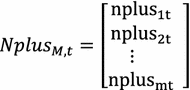

  

  Returned duplicates of machines from depot to cells in period t

• 3. The third ingredient related to the number of machine duplicates removed from cells and moved to machine depot in each period is named matrix Nminus_M,T. The components of this matrix M × 1 as shown in Fig. 3 present the number of machine duplicates which is removed from cells and moved to machine depot. nminus _jt  = a means that a duplicates of machine type j removed from cells and moved to machine depot in period t.

  Fig. 3

  

  Removed duplicates of machines from cells to depot in period t

It is worth mentioning while completing the matrices NP_M,T, Nplus_M,T and Nminus_M,T, the Constraints (13) and (14) should be considered.

• 4. The fourth ingredient related to the simultaneous assignment of duplicates of each machine type to locations and cells is named matrix $L\_C\_M_{L,C,T}$ which is a combination of the matrices [Ma_Du_Lo] and [Ce_Lo] introduced by Kia et al. (2012). The components of this matrix L × C as shown in Fig. 4 represent the assignment of machine duplicates to locations and cells, simultaneously. While completing the matrix $L\_C\_M_{L,C,T}$, Constraints (15), (16), (17) and (21) should be satisfied. After completing the matrices NP_M,T and $L\_C\_M_{L,C,t}$ for the entire periods, the values of Nplus_M,T and Nminus_M,T can be derived from Eq. (13) in each period.

  Fig. 4

  

  Assignment of machine duplicates to locations and cells

• 5. The fifth ingredient presenting the quantity of part operations assigned to the duplicates of each machine type located in locations is named matrix $P\_L\_Op\_Q_{P,L,Op,T}$ which is similar to the matrix [Pa_Op_Lo] introduced by Kia et al. (2012). This is a three-dimensional matrix P × L as shown in Fig. 5, in which each component contains k arrays (k is ${max}_p\left\{K_p\right\}$) presenting the assignment of part operations to locations. $w_{pl{k}_p}=a$ means that a quantities of part type p are processed by operation k _p on the machine located in location l. While completing the matrix $P\_L\_Op\_Q_{P,L,OP,T}$, Constraints (11) and (18)–(20) should be satisfied.

  Fig. 5

  

  Assignment of part operations to machine duplicates in locations

• 6. The sixth ingredient indicating the quantity of inventory of parts kept in period t and carried over to period t + 1 is named matrix V_P,T. The components of this matrix P × 1 as shown in Fig. 6 represent the quantity of inventory of parts kept between each two periods.v _pt  = a means that a quantities of part type p are kept in period t and carried over to period t + 1. For example, the term v₃₁ = 50 means that 50 quantities of part type 3 are kept in period 1 and carried over to period 2.

  Fig. 6

  

  The quantity of inventory of parts kept between periods

• 7. The seventh ingredient indicating the quantity of parts outsourced in period t is named matrix O_P,T. The components of this matrix P × 1 as shown in Fig. 7 represent the quantity of outsourced parts in each period. o _pt  = a means that a quantities of part type p are outsourced in period t. For example, the term of o₃₁ = 50 means that 50 quantities of part type 3 are outsourced in period 1.

  Fig. 7

  

  The quantity of outsourced parts in each period

While completing the matrices $P\_L\_Op\_Q_{P,L,OP,T}$, V _P,T and O _P,T , Eq. (12) should to be satisfied.

In general, with combining seven ingredients described above, the solution representation in each period is obtained as shown in Fig. 8. It is obvious that each solution combining seven ingredients consists of the T structure, where T is the number of periods.

Fig. 8

Solution representation in period t

Generating an initial solution

The initial solution is generated according to a hierarchical approach, in which matrices$\left[L\_C\_M_{L,C,t}\right]$, $\left[N{P}_{M,t}\right]$, $\left[Nplu{s}_{M,t}\right]$, $\left[Nminu{s}_{M,t}\right]$, $\left[P\_L\_Op\_Q_{P,L,OP,t}\right]$, $\left[V_{P,t}\right]$ and $\left[O_{P,t}\right]$ are constructed sequentially in each period by the random numbers limited in the determined interval provided that those matrices satisfy corresponding constraints. Since the matrices $\left[L\_C\_M_{L,C,t}\right]$, $\left[Nplu{s}_{M,t}\right]$, $\left[Nminu{s}_{M,t}\right]$, $\left[V_{P,t}\right]$ and $\left[O_{P,t}\right]$ have been added to the solution representation designed by Kia et al. (2013), the procedure of generating an initial solution and neighborhood generation strategy need to be modified. The generation process of initial solutions is described as follows.

In the first stage, the matrix $\left[L\_C\_M_{L,C,t}\right]$ determining how duplicates of each machine type are assigned to locations and cells is constructed. To generate a good initial solution, the number of machines of each type which is required for processing part operations is estimated roughly. This is done by considering parameters t _kpm and D _pt of each part type and randomly selecting a machine capable to process each operation of a part. Then, the components of matrix $\left[L\_C\_M_{L,C,t}\right]$ receive numbers randomly distributed between 1 and M (the number of machine types) for all periods. The number of rows is equal to the number of locations and the number of columns is equal to C_max (the maximum number of cells). Therefore, numbers in each row of matrix $\left[L\_C\_M_{L,C,t}\right]$ show the machines located in the related location in the successive periods. Also, numbers in each column present the machines assigned to related cells in successive periods.

Based on Constraint (21), each location is allowed to accommodate one machine at most. To satisfy this constraint, only one component in each row of a matrix can take a value greater than zero. After distributing these numbers in locations (rows) of matrix $\left[L\_C\_M_{L,C,t}\right]$, cell size limits should be investigated. Three cases may happen by completing matrix $\left[L\_C\_M_{L,C,t}\right]$. In the first case, the number of machines assigned to a cell (column) is less than the lower bound of that cell. In this case, that cell will not be formed and actually all assignments to that cell will be transferred to other cells. In the second case, the number of machines assigned to a cell (column) is placed between the lower and upper bounds of that cell. In this case, that cell will be formed and all assignments to that cell will be accepted. In the third case, the number of machines assigned to a cell (column) is greater than the upper bound of that cell. In this case, some extra machines are randomly chosen and moved to next cell to reach the upper bound. By this procedure, Constraints (15) and (16), related to cell size limits, are satisfied. To satisfy Constraint (18), it is required to form cells in order. For example, if cell 4 was formed while cell 2 was not formed due to cell size limits, thus the machines which had been assigned to cell 4 would be transferred to cell 2. In fact, cell 2 is formed instead of cell 4. By this simple procedure, Constraint (17) is met.

As a result, the configuration of machines in cells and assignments of locations to cells are determined by constructing of matrix $\left[L\_C\_M_{L,C,t}\right]$. Based on Eq. (13), matrices $\left[N{P}_{M,t}\right]$,$\left[Nplu{s}_{M,t}\right]$ and $\left[Nminu{s}_{M,t}\right]$ are derived from matrices $\left[L\_C\_M_{L,C,t}\right]$ which have been generated in successive periods.

After configuring cells which consists of locating machines in locations and assigning locations to cells by completing matrices $\left[L\_C\_M_{L,C,t}\right]$, part operations are assigned to the machines located in the locations by constructing the matrices $P\_L\_Op\_Q_{P,L,OP,T}$ in successive periods. While completing the matrices $P\_L\_Op\_Q_{P,L,OP,T}$, the Constraints (11) (i.e., machine process capability), (12) (i.e., part demand satisfaction), (18) (i.e., machine time capacity), and (19) and (20) (i.e., material flow conservation) should be satisfied.

Neighborhood generation strategy

Well-designed solution mutation (SM) operators are significant to the success of SA. In this research, we develop seven different (SM) operators. These are cell-number mutation operator (SM1), machine-number mutation operator (SM2), machine-inter-cell mutation operator (SM3), machine-intra-cell mutation operator (SM4), machine-location mutation operator (SM5), route-volume mutation operator (SM6) and part-operation mutation operator (SM7). To implement each one of these operators on a solution, a period is selected randomly and then the mutation operator is implemented on the selected period of solution. If implementing one mutation operator results in an infeasible solution, that solution will be eliminated. These operators are implemented on the selected period of the solution as follows.

The cell-number mutation operator (SM1) changes the number of formed cells by adding or removing a formed cell. By this operator, the only matrix $\left[L\_C\_M_{L,C,t}\right]$ is changed. Therefore, if a formed cell is removed, all machine duplicates assigned to that cell will be reassigned to the other cells randomly. In addition, if a new cell is formed, some machine duplicates assigned to the other cells will be reassigned to the newly formed cell. It is worth mentioning that the part operations processed by the randomly selected machines will be remained with them. Adding or removing a cell needs updating matrix $\left[L\_C\_M_{L,C,t}\right]$ and can influence terms (1), (2), (7) and (10) of the objective function.

The machine-number mutation operator (SM2) changes the matrices $\left[N{P}_{M,t}\right]$, $\left[Nplu{s}_{M,t}\right]$ and $\left[Nminu{s}_{M,t}\right]$ by adding or removing a duplicate of a machine type or concurrently removing a duplicate of a machine type and then adding a duplicate of another machine type. Implementing this operator might need updating all matrices and can influence all terms of the objective function.

The machine-inter-cell mutation operator (SM3) randomly selects two different filled columns of matrix $\left[L\_C\_M_{L,C,t}\right]$ and substitute their values. In this way, different machine duplicates assigned to different cells are substituted between cells. The machine-intra-cell mutation operator (SM4) randomly selects a filled column of matrix $\left[L\_C\_M_{L,C,t}\right]$ and substitutes its values. In this way, different machine duplicates assigned to different locations of a cell are substituted. The machine-location mutation operator (SM5) randomly selects two different filled rows of matrix $\left[L\_C\_M_{L,C,t}\right]$ and substitutes their values. In this way, different machine duplicates assigned to different locations are substituted. Implementing these operators needs updating matrices $\left[L\_C\_M_{L,C,t}\right]$ and $\left[P\_L\_Op\_Q_{P,L,OP,t}\right]$ and can influence terms (1)–(3) and (10) of the objective function.

The route-volume mutation operator (SM6) changes the matrices $\left[P\_L\_Op\_Q_{P,L,Op,t}\right]$, $\left[V_{P,t}\right]$ and $\left[O_{P,t}\right]$ by increasing or decreasing the production lot volumes of some defined routes for a part which results in modification of internal production volume of that part or concurrently decreasing a portion of a production lot and then increasing same volume to another production lot. This operator can influence terms (1), (2), (6) and (8)–(10). The part-operation mutation operator (SM7) changes the matrix $\left[P\_L\_Op\_Q_{P,L,Op,t}\right]$ by selecting an operation of a part and changing the machine assigned to process that operation. This operator can influence terms (1), (2), (6) and (10) of the objective function.

Clustering the archive solutions

Clustering of the solutions in the archive where the non-dominated solutions obtained so far are stored is employed in AMOSA algorithm in order to explicitly compel the diversity of the non-dominated solutions and keep the archive size under a given upper bound. As it was revealed by Bandyopadhyay et al. (2008), the most time-consuming part in AMOSA algorithm is the clustering procedure which is based on single linkage algorithm (Jain and Dubes 1988). Here, we use a simple elimination method to remove extra solutions from the archive instead of single linkage algorithm and avoid its complexity. Whenever the number of solutions in archive becomes more than upper bound, a surrounding rectangle is made by two neighbor solutions for each solution except those in extreme points. A rectangle with smaller area shows greater crowded region in archive. Then, the solution surrounded by the smallest rectangle area is eliminated to increase the uniformity in the archive and meet limit on archive size.

Amount of domination

The concept of amount of domination is used for computing the acceptance probability of a new solution in AMOSA. By considering two solutions x and y, the amount of domination is calculated as $\mathit{\Delta }{\text{dom}}_{x,y}={\prod }_{i=1,Z_i\left(x\right)\ne Z_i\left(y\right)}^M\left(\left|Z_i\left(x\right)-Z_i\left(y\right)/R_i\right|\right)$, where M = number of objective functions and R _i is the range of the ith objective. In our model, M = 2 and the solutions present in the archive are used for computing R _i .

Acceptance/rejection mechanism of a neighborhood solution based on AMOSA

One of the solutions, called current-sol, is randomly selected as the initial solution at temperature T₀ from Archive. The current-sol is mutated to generate a new solution called new-sol. The domination status of new-sol is examined with regard to the current-sol and solutions in the archive. Based on the domination status between current-sol and new-sol, three different cases may happen. These are described below.

Case 1: current-sol dominates the new-pt and k solutions from the Archive dominate the new-sol. In this case, the new-sol is accepted as the current-sol with

$$\text{Probability}=\frac{1}{1+exp(\mathit{\Delta }{\text{dom}}_{\text{avg}}\times T)}$$

(24)

where $\mathit{\Delta }{\text{dom}}_{\text{avg}}=\left(\left({\sum }_{i=1}^k\mathit{\Delta }{\text{dom}}_{i,\text{new - sol}}\right)+\mathit{\Delta }{\text{dom}}_{\text{current - sol},\text{new - sol}}\right)/\left(k+1\right)$. Note that Δdom_avg denotes the average amount of domination of the new-sol by (k + 1) solutions, namely, the current-sol and k solutions of the archive.

Case2: current-sol and new-sol are non-dominating with respect to each other. Now, based on the domination status of new-sol and solutions of archive, the following three situations may happen.

• 1. new-sol is dominated by k solutions in the archive where k ≥ 1. The new-sol is selected as the current-sol with

$$\text{Probability}=\frac{1}{1+exp(\mathit{\Delta }{\text{dom}}_{\text{avg}}\times T)}$$

(25)

where $\mathit{\Delta }{\text{dom}}_{\text{avg}}={\sum }_{i=1}^k\mathit{\Delta }{\text{dom}}_{i,\text{new - sol}}/k$ .

• 2. new-sol is also non-dominating with regard to the other solutions in the archive. In this case, the new-sol is on the same front as the archive. Therefore, the new-sol is accepted as the current-sol and added to the archive. If the archive becomes overfull, proposed elimination method is performed to reduce the number of solutions to archive size.

• 3. new-sol dominates points of the archive. Again, the new-sol is selected as the current-sol, and added to the Archive. All the dominated solutions are removed from the archive.

Case 3: new-sol dominates current-sol. Here, based on the domination status of new-sol and solutions of archive, the following three situations may happen.

• 1. new-sol dominates the current-sol but k(k ≥ 1) solutions in the archive dominate this new-sol. Note that this situation may happen only if the current-sol is not a member of the archive. Here, the minimum of the difference of domination quantities between the new-sol and the k solutions, denoted by Δdom_min, of the archive is calculated. The solution from the archive which corresponds to the minimum difference is selected as the current-sol with $\text{Probability}=1/\left(1+exp\left(-\mathit{\Delta }{\text{dom}}_{\text{min}}\right)\right).$ Otherwise, the new-sol is accepted as the current-sol.

• 2. new-sol is non-dominating with regard to the solutions in the archive except the current-sol if it belongs to the archive. Thus new-sol, which is now accepted as the current-sol, can be considered as a new non-dominated solution that must be added to archive. If the current-sol is in the archive, then it is removed. Otherwise, if the number of points in the archive becomes more than the archive size, elimination method is performed to reduce the number of points to archive size.

• 3. new-sol also dominates k(k ≥ 1), other solutions, in the archive. Thus, the new-sol is accepted as the current-sol and added to the archive, while all the dominated solutions of the archive are removed.

The above process is repeated Markov chain length (MCL) times for each temperature T. Temperature is reduced to α·T, using the cooling rate of α till the minimum temperature T_f is attained. The process thereafter stops, and the archive containing the final non-dominated solutions is reported.

NSGA-II

Here, a brief description of employed non-dominated sorting genetic algorithm II (NSGA-II) is explained. At first, a random parent population P₀ of size N is created by the procedure described in “Generating and initial solution”. The non-dominated fronts F₁, F₂,…, F _k are identified by using the fast non-dominated sorting algorithm defined by Deb et al. (2002). Offspring population Q₀ of size N is created by using binary tournament selection operator, crossover operators and mutation operators. Thereafter, two populations P₀ and Q₀ are combined together to form a new population R _t of size 2N. Then, a non-dominated sorting is performed on R _t to identify different fronts. Next, making up the new population P _t of size N starts with filling up by the first non-domination front and continues with solutions of the second non-domination front, and so forth. Since all fronts cannot be accommodated in N slots available for the new population P _t , the solutions of the last front that cannot be completely accommodated are realized in the descending order of their crowding distance values and solutions from the top of the ordered list are chosen to be accommodated in the population P _t . Now, offspring population Q_t+1 of size N is created from population P_t+1 by using the tournament selection, crossover, and mutation operators. In a similar way, two new populations P_t+1 and Q_t+1 are combined to form a new population R_t+1 of size 2N and these steps are repeated until the stopping criterion is satisfied. In this case, the algorithm terminates if the computational time for successive generations exceeds the specific time.

Computational results for multi-objective model by AMOSA

Assessing the ability of AMOSA to reach true Pareto-optimal

At first, to investigate the performance of the developed AMOSA algorithm to reach optimal Pareto front, the efficient solutions obtained by ∈-constraint method as an exact method for the three numerical examples are compared with the best Pareto solutions obtained by AMOSA. Since the input data and the solutions obtained by GAMS software for these examples have been given by Kia et al. (2013), they are not repeated here.

The extended AMOSA algorithm have been coded in MATLAB R2010a and executed on an Intel^® CoreTM 2.66 GHz Personal Computer with 4 GB RAM. We have chosen a reasonable set of values in respect to some experiments which were executed with various parameters-sets. Extensive experiments are suggested for future studies. For the designed AMOSA, the cooling rate, archive size, initial temperature, final temperature and MCL are set as 0.99, 20, 100,000, 100, and 200, respectively.

Tables 2 and 3 present the non-dominated solutions obtained by AMOSA algorithm and ∈-constraint method in solving three examples.

Table 2 Pareto solutions obtained by AMOSA algorithm for the three examples

Table 3 Pareto solutions obtained by ∈-constraint method for the three examples

To compare the results of AMOSA algorithm and ∈-constraint method on three test problems, we use four well-known metrics in the literature (Okabe et al. 2003), which are briefly explained as follows.

Number of non-dominated solutions (N)

In this respect, the algorithm with more non-dominated solutions in a shorter time has a better performance.

Maximum spread (Max_spread)

This metric shows the span of Pareto front obtained by the algorithm. Obviously, the larger Max_spread is preferred. It is calculated by:

$${\text{Max}}_{\text{spread}}=\sqrt{{\sum }_{t=1}^T{\left(\text{min}{f}_t-\text{max}{f}_t\right)}^2}$$

(26)

where T is the number of objective functions (i.e., 2) and f _t is the value of tth objective function.

Spacing

This metric measures the range (distance) variance of adjacent solutions in the Pareto front. As a result, the smaller value of spacing indicates more uniformity of solutions in Pareto front and would be more desirable. Equation (27) calculates the third metric.

$$\text{Spacing}=\sqrt{1/n-1{\sum }_{i=1}^n{\left(d_i-\overline{d}\right)}^2}$$

(27)

where $d_i={min}_j\left(\left|f_1^i-f_1^j\right|+\left|f_2^i-f_2^j\right|\right),i,j=1,\dots ,n,$$\overline{d}$ is the average of all d _i and n is the number of non-dominated solutions.

Time

Obviously, the algorithm with the smaller value of execution time is more desirable.

In Table 4, the performance metrics obtained by AMOSA algorithm and ∈-constraint method are presented for three examples. As can be seen, AMOSA algorithm has found more non-dominated solutions (N) in solving all three examples which brings more flexibility for the system designer to make decision among more alternatives.

Table 4 Comparison between AMOSA algorithm and ∈-constraint method for the three examples

The obtained values for performance metric (Max_spread) in all three examples also show more extension of Pareto front obtained by AMOSA in compare to ∈-constraint method. This is another advantage of the designed solution approach.

Nevertheless, in regard to performance metric (Spacing) it should be admitted that the values obtained by AMOSA algorithm are not as satisfactory as those obtained by ∈-constraint method as true Pareto front. Although, it is worth mentioning that uniformity of solutions is determined by system designer in ∈-constraint method. Hence, more uniformity is observed for the non-dominated solutions obtained by ∈-constraint method. Considering the fact the number of the non-dominated solutions obtained by AMOSA algorithm is much more than those obtained by ∈-constraint method, there is possibility to eliminate some neighbor solutions in a crowded region of Pareto set to reduce the amount of performance metric (spacing) and improve the performance of AMOSA in this aspect. Regarding the performance metric time, it is clear that computational time of AMOSA is much lesser than ∈-constraint method. This is another achievement of the designed AMOSA in reaching solutions near true Pareto front in solving NP-hard proposed model.

As the required time to obtain an optimal solution from true Pareto front by GAMS is too long for the first and second example, to save computation effort each run is interrupted on a predetermined time and the solution obtained so far is reported. As a result, the obtained solutions might not belong to true Pareto front. However, for the third example finding the optimal solution has been possible by eliminating alternative routings feature from the main model.

Considering the optimality status of the obtained Pareto front by ∈-constraint method as described above, the quality of non-dominated solutions obtained by AMOSA and ∈-constraint method is compared through Figs. 9, 10 and 11. As it is revealed by Figs. 9 and 10, the Pareto front obtained by AMOSA is closer to true Pareto front than one obtained by∈-constraint method. Comparing the computational time of two methods proves the remarkable achievement of the designed AMOSA in solving an NP-hard problem.

Fig. 9

Pareto front obtained by AMOSA algorithm and ∈-constraint method for example 1

Fig. 10

Pareto front obtained by AMOSA algorithm and ∈-constraint method for example 2

Fig. 11

Pareto front obtained by AMOSA algorithm and ∈-constraint method for example 3

By comparing Pareto fronts obtained for example 3 in Fig. 11, it can be seen that the non-dominated solutions delivered by AMOSA are in a short distance to true Pareto front obtained by GAMS. The relative gap for non-dominated solutions which are close to each other in both Pareto fronts is around 5 %. This can be regarded as a satisfactory result. By considering Figs. 9, 10 and 11, the concept of multi-objective approach can be also revealed easily. The decision-maker should choose one of these alternatives: lower costs and higher cell workload imbalance or more costs and more even cell workload.

Comparison between AMOSA, NSGA-II and ∈-constraint method

In this section, 12 numerical examples are solved using the extended AMOSA to evaluate its computational efficiency in terms of performance metrics defined above. The obtained solutions by AMOSA are compared with those obtained by NSGA-II and ∈-constraint and shown in Table 5. For better comparison, Quality metric defined as below is replaced with the metric number of non-dominated solutions (N).

Table 5 Comparison between AMOSA, NSGA-II and ∈-constraint method

Quality metric (QM)

It calculates the fraction of solutions from a particular method that remains non-dominating when the final Pareto solutions obtained from all the algorithms are combined. A value near 1 indicates better performance, whereas a value near 0 indicates poorer performance. Based on this metric, the algorithm that finds more Pareto-optimal solutions has a better performance. However, some Pareto solutions of an algorithm may be dominated by those obtained by the other algorithms. Hence, the number of final non-dominated solutions obtained by each algorithm is important to calculate this metric (Bandyopadhyay et al. 2004).

As it has been reported in the literature, an effective cooling schedule is essential for reducing the amount of time required by the algorithm to find an optimal solution. But cooling schedules are almost always heuristic and it would be needed to balance moderately the computational time with the simulated annealing dependence on problem size.

The simulated annealing schedule is defined by initial temperatures in points [30,000, 50,000, 100,000, 150,000], a MCL in points [30, 50, 200] and final temperatures set to 100 as well as a cooling rate α = 0.995.

Because of exponential reduction of error probability, several short-term runs of SA results better than a long-term one (Defersha and Chen 2008a, b). Hence, each run has been repeated 5 times to solve each example and the best obtained solution among them has been reported.

Since there are numerous decision variables and constraints in the proposed model, some of the numerical examples cannot be solved in a reasonable time by GAMS. Therefore, the solving process will be continued until the GAMS software encounters a resource limit as an out of memory message. At this point, the best obtained value of objective function is reported as Pareto solutions to be compared with AMOSA.

For the examples 5–11, GAMS is interrupted because of out of memory predicament. As a result, the obtained Pareto solutions for those examples are not optimal. Generating numerical examples is stopped at example 12, as the solution space is enlarged so much that GAMS even cannot generate a feasible solution before encountering out of memory message.

The computational results corresponding to the defined four performance metrics for the 12 different numerical examples are presented in Table 5. We have compared the encoded AMOSA with the NSGA-II and ∈-constraint method.

In NSGA-II, the crossover probability is kept equal to 0.9. Here, the population size in NSGA-II is set to 100. Maximum iterations for NSGA-II are 500.

The quality metric, maximum spread and spacing values obtained using the three methods are discussed as follows. AMOSA performs the best for example problems 6–12 in terms of quality metric. The ∈-constraint performs well for example problems 1–5.

AMOSA is giving the best performance of maximum spread all the times, while ∈-constraint performs the worst. It is seen that AMOSA takes less time in almost all examples because of its smaller complexity. However, the performance of AMOSA is not satisfactory in terms of spacing metric in compare to ∈-constraint method.

Conclusion

A solution approach based on simulated annealing algorithm was employed to solve a multi-objective mixed-integer non-linear programming (MINLP) model integrating CF, GL and PP decisions under a dynamic environment. Incorporating design features including alternative process routings, operation sequence, processing time, production volume of parts, purchasing machine, duplicate machines, machine capacity, lot splitting, group layout, multi-rows layout of equal area facilities, flexible reconfiguration, machine depot, variable number of cells, balancing cell workload, outsourcing and inventory holding of parts in a multi-objective model is one of the advantages of the integrated model.

The extended model was capable to determine optimally the production volume of alternative processing routes of each part, the material flow happening between different machines, the cell configuration, the machine locations, the number of formed cells, the number of purchased machines, the number of machines kept in depot, the production plan for each part type by satisfying demand through internal production, outsourcing and inventory holding.

Since the extended multi-objective model belongs to NP-hard problems, an archived multi-objective simulated annealing (AMOSA) with an effective solution structure and seven mutation operators has been developed to solve the extended model and produce non-dominated solutions. In this study, a heuristic hierarchical procedure was designed to generate the initial solutions with good quality. In addition, the solution structure was presented as a matrix with seven ingredients fulfilled hierarchically to satisfy all constraints and successive neighbor solutions are produced from the initial solution by implementing elaborately designed mutation operators. All components in the objective functions could be influenced by designed operators to more exploration and exploitation of solution space. The computational results showed that the developed AMOSA had the satisfactory performance in reaching Pareto solutions in comparison to NSGA-II and ∈-constraint method based on some comparison metrics.

Incorporating other features, such as introducing uncertainty in part demands, machine time capacity and cost coefficients, integrating with reliability and labor issues, designing layout of unequal-area facilities, implementing extensive experiments for problem tuning, and solving more numerical examples especially in real cases will be left to future research.

References

Aramoon Bajestani M, Rabbani M, Rahimi-Vahed AR, Baharian Khoshkhou G (2009) A multi-objective scatter search for a dynamic cell formation problem. Comput Oper Res 36:777–794
Bandyopadhyay S, Pal SK, Aruna B (2004) Multi-objective GAs, quantitative indices and pattern classification. IEEE Trans Syst Man Cybernet B 34(5):2088–2099
Bandyopadhyay S, Saha S, Maulik U, Deb K (2008) A simulated annealing-based multiobjective optimization algorithm: AMOSA. IEEE Trans Evol Comput 12(3):269–283
Benjafaar S, Heragu S, Irani S (2002) Next generation factory layouts: research challenges and recent progress. Interfaces 32(6):58–76
Coello Coello CA (2005) Evolutionary multiobjective optimization: recent trends in evolutionary multiobjective optimization. Springer, Berlin
Deb K, Pratap A, Agarwal S, Meyarivan T (2002) A fast and elitist multi-objective genetic algorithm: NSGA-II. IEEE Trans Evol Comput 6(2):182–197
Defersha FM, Chen M (2008a) A parallel multiple Markov chain simulated annealing for multi-period manufacturing cell formation problems. Int J Adv Manuf Technol 37:140–156
Defersha FM, Chen M (2008b) A parallel genetic algorithm for dynamic cell formation in cellular manufacturing systems. Int J Prod Res 46:6389–6413
Defersha FM, Chen M (2009) Simulated annealing algorithm for dynamic system reconfiguration and production planning in cellular manufacturing. Int J Manuf Technol Manag 17(1/2):103–124
Dimopoulos C (2007) Explicit consideration of multiple objectives in cellular manufacturing. Eng Optim 39(5):551–565
Drolet J, Marcoux Y, Abdulnour G (2008) Simulation-based performance comparison between dynamic cells, classical cells and job shops: a case study. Int J Prod Res 46(2):509–536
Eiben AE, Smith JE (2003) Introduction to evolutionary computing. Springer, Berlin
Fonseca CM, Fleming PJ (1995) Multi-objective genetic algorithms made easy: selection, sharing and mating restriction. In: First IEE/IEEE international conference on genetic algorithms in engineering systems, Sheffield, England
Ghotboddini MM, Rabbani M, Rahimian H (2011) A comprehensive dynamic cell formation design: Benders’ decomposition approach. Expert Syst Appl 38:2478–2488
Hsu CM, Su CT (1998) Multi-objective machine-component grouping in cellular manufacturing: a genetic algorithm. Prod Plan Control 9(2):155–166
Jain AK, Dubes RC (1988) Algorithms for clustering data. Prentice-Hall, Englewood Cliffs
Javadian N, Aghajani A, Rezaeian J, Ghaneian Sebdani MJ (2011) A multi-objective integrated cellular manufacturing systems design with dynamic system reconfiguration. Int J Adv Manuf Technol 56:307–317
Kia R (2014) Multi-objective optimization of dynamic cellular manufacturing systems integrated with layout problems. PhD Dissertation, Department of Industrial Engineering, Mazandaran University of Science and Technology, Babol, Iran
Kia R, Baboli A, Javadian N, Tavakkoli-Moghaddam R, Kazemi M, Khorrami J (2012) Solving a group layout design model of a dynamic cellular manufacturing system with alternative process routings, lot splitting and flexible reconfiguration by simulated annealing. Comput Oper Res 39:2642–2658
Kia R, Shirazi H, Javadian N, Tavakkoli-Moghaddam R (2013) A multi-objective model for designing a group layout of a dynamic cellular manufacturing system. J Ind Eng Int 9:8
Kim CO, Baek JG, Jun J (2005) A machine cell formation algorithm for simultaneously minimizing machine workload imbalances and inter-cell part movements. Int J Adv Manuf Technol 26(3):268–275
Kirkpatrick S, Gelatt CD, Vecchi MP (1983) Optimization by simulated annealing. Science 220:671–680
Knowles J, Corne D (1999) The Pareto archived evolution strategy: a new baseline algorithm for multi-objective optimization. Proceedings of the 1999 congress on evolutionary computation. IEEE Press, Piscataway, pp 98–105
Lee SD, Chen YL (1997) A weighted approach for cellular manufacturing design: minimizing intercell movement and balancing workload among duplicated machines. Int J Prod Res 35(4):1125–1146
Lei D, Wu Z (2005) Tabu search-based approach to multi-objective machine-part cell formation. Int J Prod Res 43(24):5241–5252
Majazi Dalfard V (2013) New mathematical model for problem of dynamic cell formation based on number and average length of intra and intercellular movements. Appl Math Model 37(4):1884–1896
Malakooti B, Yang Z (2002) Multiple criteria approach and generation of efficient alternatives for machine-part family formation in group technology. IIE Trans 34:837–846
Mansouri SA, Moattar-Husseini SH, Zegordi SH (2003) A genetic algorithm for multiple objective dealing with exceptional elements in cellular manufacturing. Prod Plan Control 14(5):437–446
Mungwattana A (2000) Design of cellular manufacturing systems for dynamic and uncertain production requirements with presence of routing flexibility. Ph.D. Thesis submitted to the Faculty of the Virginia Polytechnic Institute and State University, Blackburg
Okabe T, Jin Y, Sendhoff B (2003) A critical survey of performance indices for multiobjective optimization. CEC ‘03 2003 Congress Evol Comput 2:878–885
Pattanaik LN, Jain PK, Mehta NK (2007) Cell formation in the presence of reconfigurable machines. Int J Adv Manuf Technol 34:335–345
Prabhaharan G, Muruganandam A, Asokan P, Girish BS (2005) Machine cell formation for cellular manufacturing systems using an ant colony system approach. Int J Adv Manuf Technol 25:1013–1019
Rheault M, Drolet J, Abdulnour G (1995) Physically reconfigurable virtual cells: a dynamic model for a highly dynamic environment. Comput Ind Eng 29(1–4):221–225
Safaei N, Tavakkoli-Moghaddam R (2009) Integrated multi-period cell formation and subcontracting production planning in dynamic cellular manufacturing. Int J Prod Econ 120(2):301–314
Safaei N, Saidi-Mehrabad M, Jabal-Ameli MS (2008) A hybrid simulated annealing for solving an extended model of dynamic cellular manufacturing system. Eur J Oper Res 185:563–592
Schaffer J (1985) Multiple objective optimization with vector evaluated genetic algorithms. In: First international conference on genetic algorithms, Pittsburgh
Shanker R, Vrat P (1999) Some design issues in cellular manufacturing using the fuzzy programming approach. Int J Prod Res 37(11):2545–2563
Solimanpur M, Vrat P, Shankar R (2004) A multi-objective genetic algorithm approach to the design of cellular manufacturing systems. Int J Prod Res 42(7):1419–1441
Su CT, Hsu CM (1998) Multi-objective machine-part cell formation through parallel simulated annealing. Int J Prod Res 36(8):2185–2207
Suppapitnarm A, Seffen KA, Parks GT, Clarkson PJ, Liu JS (1999) Design by multi-objective optimization using simulated annealing. In: First international conference on engineering design ICED 99, Munich, Germany
Suresh NC, Slomp J (2001) A multi-objective procedure for labour assignments and grouping in capacitated cell formation problems. Int J Prod Res 39(18):4103–4131
Tavakkoli-Moghaddam R, Ranjbar-Bourani M, Amin GR, Siadat A (2010) A cell formation problem considering machine utilization and alternative process routes by scatter search. J Intell Manuf 23(4):1127–1139
Van Veldhuizen DA, Lamont G (2000) Multiobjective evolutionary algorithms: analyzing the state-of-the-art. Evol Comput 8:125–147
Wang X, Tang J, Yung KL (2009) Optimization of the multi-objective dynamic cell formation problem using a scatter search approach. Int J Adv Manuf Technol 44:318–329
Wemmerlov U, Hyer NL (1986) Procedures for the part family/machine group identification problem in cellular manufacture. J Oper Manag 6:125–147
Wemmerlov U, Johnson DJ (2000) Empirical findings in manufacturing cell design. Int J Prod Res 38:481–507
Yasuda K, Hu L, Yin Y (2005) A grouping genetic algorithm for the multi-objective cell formation problem. Int J Prod Res 43(4):829–853
Zitzler E, Laumanns M, Thiele L (2001) SPEA2: improving the strength Pareto evolutionary algorithm. In: Giannakoglou K, Tsahalis D, Periaux J, Papailou P, Fogarty T (eds) EUROGEN, evolutionary methods for design, optimization and control with applications to industrial problems. Athens, pp 95–100
Acknowledgments
This work was financially supported by Islamic Azad University, Qom Branch, grant number 12006.
Author information
Authors and Affiliations
Corresponding author
Rights and permissions
Open Access This article is distributed under the terms of the Creative Commons Attribution License which permits any use, distribution, and reproduction in any medium, provided the original author(s) and the source are credited.
About this article
Cite this article
Shirazi, H., Kia, R., Javadian, N. et al. An archived multi-objective simulated annealing for a dynamic cellular manufacturing system. J Ind Eng Int 10, 58 (2014). https://doi.org/10.1007/s40092-014-0058-6
Received:
Accepted:
Published:
DOI: https://doi.org/10.1007/s40092-014-0058-6