On the relative K-group in the ETNC, Part II

Abstract

In a previous paper we showed that, under some assumptions, the relative K-group in the Burns–Flach formulation of the equivariant Tamagawa number conjecture (ETNC) is canonically isomorphic to a K-group of locally compact equivariant modules. Our approach as well as the standard one both involve presentations: One due to Bass–Swan, applied to categories of finitely generated projective modules; and one due to Nenashev, applied to our topological modules without finite generation assumptions. In this paper we provide an explicit isomorphism.

1 Introduction

The equivariant Tamagawa number conjecture (ETNC) for possibly non-commutative coefficients postulates the equality of two elements in a certain K-theory group. We shall recall the wider background of the conjecture below in Sect. 2, or see Burns–Flach [1, Sect. 4.3, Conjecture 4].

Let A be a finite-dimensional semisimple ${\mathbb {Q}}$-algebra and ${\mathfrak {A}}\subset A$ an order. We write $A_{{\mathbb {R}}}:=A\otimes _{{\mathbb {Q}}}{\mathbb {R}}$. Let $K_{n}(-)$ denote n-th K-group. Only $K_{0}$ and $K_{1}$ are truly important for this article. By general principles, there is a long exact sequence

$$\begin{aligned} \cdots \longrightarrow K_{1}({\mathfrak {A}})\longrightarrow K_{1}(A_{{\mathbb {R}} })\longrightarrow K_{0}({\mathfrak {A}},{\mathbb {R}})\longrightarrow K_{0} ({\mathfrak {A}})\longrightarrow \cdots \text {,} \end{aligned}$$

(1.1)

where $K_{n}({\mathfrak {A}},{\mathbb {R}})$ denotes certain groups which are designed to make this sequence exact. These groups are called ‘relative K-theory’, but there is not much behind it. They simply come from the fiber belonging to the map between the other two K-theory spectra involved in the sequence.

In the previous paper [5] we have shown, assuming ${\mathfrak {A}}$ to be regular, that there is a canonical isomorphism

$$\begin{aligned} K_{n}({\mathfrak {A}},{\mathbb {R}})\cong K_{n+1}(\mathsf {LCA}_{{\mathfrak {A}} })\text {,} \end{aligned}$$

(1.2)

where $\mathsf {LCA}_{{\mathfrak {A}}}$ is the exact category of locally compact ${\mathfrak {A}}$-modules: Its objects are locally compact topological right ${\mathfrak {A}}$-modules, morphisms are continuous ${\mathfrak {A}}$-module morphisms. There is no finite generation assumption. The exact structure is such that admissible monics are the closed injections, and admissible epics are the open surjections. For example, this implies that cokernels in this category always carry precisely the quotient topology. The category is not abelian, but it has all kernels and cokernels.

We are mostly interested in the case $n=0$. In the formulation of the ETNC in [1], the equivariant Tamagawa numbers live in the relative K-group $K_{0}({\mathfrak {A}},{\mathbb {R}})$. This group has an explicit presentation due to Bass and Swan, based on generators

$$\begin{aligned}{}[P,\varphi ,Q]\text {,} \end{aligned}$$

where P, Q are finitely generated projective right ${\mathfrak {A}}$-modules and $\varphi :P_{{\mathbb {R}}}\overset{\sim }{\rightarrow }Q_{{\mathbb {R}}}$ an isomorphism; modulo some relations. On the other hand, the group $K_{1}(\mathsf {LCA}_{{\mathfrak {A}}})$ has an explicit presentation due to Nenashev, based on double exact sequences

where A, B, C are locally compact right ${\mathfrak {A}}$-modules; modulo some other relations. This datum corresponds to a closed loop in the K-theory space.

Main Theorem

Let A be a finite-dimensional semisimple ${\mathbb {Q}}$-algebra and ${\mathfrak {A}}\subset A$ an order. Then the map

$$\begin{aligned} \vartheta :K_{0}({\mathfrak {A}},{\mathbb {R}})\longrightarrow K_{1}(\mathsf {LCA} _{{\mathfrak {A}}}) \end{aligned}$$

(1.3)

sending $[P,\varphi ,Q]$ to the double exact sequence $\left\langle \left\langle P,\varphi ,Q\right\rangle \right\rangle$ (described below) is a well-defined morphism from the Bass–Swan to the Nenashev presentation. If ${\mathfrak {A}}$ is regular, then the map $\vartheta$ is an isomorphism.

Here is how we build $\vartheta$: Given $[P,\varphi ,Q]$, we define the aforementioned double exact sequence $\left\langle \left\langle P,\varphi ,Q\right\rangle \right\rangle$ to be

where P carries the discrete topology, $P_{{\mathbb {R}}}$ the real vector space topology, and $T_{P}:=P_{{\mathbb {R}}}/P$ carries the torus quotient topology (correspondingly for Q). The products and direct sums are indexed over ${\mathbb {Z}}_{\ge 0}$. The four morphisms are complicated to define: They arise as the sum of various maps, which can be depicted as

where we read the objects in the left (resp. middle, right) column as the direct summands appearing in the left (resp. middle, right) term of the double exact sequence. The solid versus dotted lines indicate which side of the double exact sequence they belong to. Each of the arrows without a label only depends on P and Q, but not on $\varphi$. We refer to Sect. 4 for details. We only gave these brief indications to give an impression what kind of object we are dealing with.

The mere existence of the map $\vartheta$ (not needing ${\mathfrak {A}}$ regular) will be Theorem 4.1 and is independent of the previous paper [5]. The proof that it is an isomorphism will be Theorem 5.1. The latter is a lot harder and will require us to work with some explicit simplicial model of K-theory, based on the work of Gillet and Grayson. A variant which works for ${\mathfrak {A}}$ a Gorenstein order (instead of regular) will be provided in the sequel [6, Theorem 3].

2 Background on the bigger picture

The (proven) classical Tamagawa number conjecture of Weil, put forward around 1960, implies in a rather elementary special case the formula

$$\begin{aligned} \mu _{\infty }\left( {\text {SL}}_{2}({\mathbb {Z}})\backslash \text {SL}_{2}({\mathbb {R}}) \right) \cdot \prod _{p} \mu _{p}(\text {SL}_{2}({\mathbb {Z}}_{p}))=1\text {,} \end{aligned}$$

(2.1)

where p runs over all prime numbers and $\mu _{(-)}$ are Haar measures on the locally compact groups $\text {SL}_{2}({\mathbb {R}})$ resp. $\text {SL}_{2}({\mathbb {Q}}_{p})$.

Haar measures are only well-defined up to a positive real multiple, but by interpreting the above appearances of ${\mathbb {Q}}_{p}$ and ${\mathbb {R}}$ in terms of the adelic points of the group $\text {SL}_{2}$, another locally compact group, one can set up a truly canonical measure not depending on any choices—the so-called ‘Tamagawa measure’.

Either way: Upon evaluating the above volumes, Formula 2.1 simplifies to

$$\begin{aligned} \left( \frac{\pi ^{2}}{6}\right) \cdot \prod _{p}\left( 1-p^{-2}\right) =1\text {,}\qquad \qquad \text {i.e.,}\qquad \qquad \frac{\pi ^{2}}{6}\cdot \zeta (2)^{-1}=1\text {,} \end{aligned}$$

(2.2)

where $\zeta$ is the zeta function of the number field ${\mathbb {Q}}$, i.e., the classical Riemann zeta function.

This formula is of course famous. One could say that the above volume computation for $\text {SL}_{2}$ interprets each factor $1-p^{-2}$ as coming from something p-adic, and $\zeta (2)=\pi ^{2}/6$ as arising from the reals.

The idea behind Weil’s conjecture was that variants of this formula should hold for any semisimple algebraic group instead of just $\text {SL} _{2}$, and for all number fields instead of ${\mathbb {Q}}$. The zeta function has to be replaced by the one of the number field. Instead of all primes p we would run over all prime ideals $\mathfrak {p}$ of the ring of integers, i.e., the finite places, and the appearance of ${\mathbb {R}}$ would be replaced by the infinite places of the number field. Some additional factors enter. This form of the Tamagawa number conjecture is fully proven. See [16].

Now one can have a bold idea: While the above conjecture is only concerned with linear algebraic groups, an elliptic curve also gives a group variety. Could such a formula still hold? This great philosophical idea is due to Birch and Swinnerton–Dyer [8] in order to interpret their computer experiments and famous conjecture from [7]. Later, Bloch [4] perfected this picture and showed that the Tamagawa number conjecture for certain group varieties is entirely equivalent to the full Birch–Swinnerton–Dyer conjecture (BSD) for abelian varieties. The role of the zeta function in Eq. (2.2) is taken by the L-function of the abelian variety.

The ETNC now goes well beyond this idea: One replaces the abelian variety by an arbitrary motive. This is sensible because really an L-function is attached to a motive. In a very simplified form, one could say that the role of the real numbers ${\mathbb {R}}$ in Eq. (2.1) is taken over by the Betti realization, and the individual factors at primes p correspond to p-adic realizations of the motive. Vaguely speaking, the analogue of $\text {SL}_{2}({\mathbb {Z}})$ in Formula 2.1 are motivic cohomology groups. For example, a rudimentary form of the BSD conjecture relates the order of vanishing of the L-function of the abelian variety at $s=1$ to the rank of its Mordell–Weil group of rational points, but the latter can also be expressed as the rank of a motivic cohomology group. The transition to motives is due to Bloch and Kato [3] (and refines conjectures of Deligne and Beilinson), and along a chain of developments due to (among others) Fontaine, Perrin–Riou (e.g., [10]), and Kato, led to the equivariant formulation of Burns and Flach [1, Sect. 4.3]. In all these variations the goal always remains to relate special L-values to other invariants.

After this general outlook, where we have seen the vital role played by real and p-adic topologies, let us return to how Sequence 1.1 enters the story. This is the part of the conjecture relevant for what we want to explain in the present article. Most of the above summary only describes the non-equivariant setting. In Eq. (1.1) the latter corresponds to $A:={\mathbb {Q}}$ and ${\mathfrak {A}}:={\mathbb {Z}}$ (“trivial action”). The sequence then simplifies to

$$\begin{aligned} \cdots \longrightarrow \{\pm 1\}\longrightarrow {\mathbb {R}}^{\times }\longrightarrow K_{0}({\mathfrak {A}},{\mathbb {R}})\overset{0}{\longrightarrow }{\mathbb {Z}} \longrightarrow \cdots \end{aligned}$$

and thus under the absolute value map, we get a canonical isomorphism

$$\begin{aligned} K_{0}({\mathfrak {A}},{\mathbb {R}})\simeq {\mathbb {R}}_{>0}^{\times } \end{aligned}$$

identifying the relative K-group with the positive real numbers. In this special case the ETNC is a conjecture about the equality of two elements in ${\mathbb {R}}_{>0}^{\times }$, a rather coarse invariant. Following the narrative of [3], one can really imagine this as just comparing volumes; much like in the classical Tamagawa number conjecture of Weil and Eq. (2.1). However, in the general equivariant setting, the ETNC is a much more precise statement. The group $K_{0}({\mathfrak {A}},{\mathbb {R}})$ will have a much richer structure, and thus the equality of two of its elements is a more refined prediction.

One now constructs the two elements in $K_{0}({\mathfrak {A}},{\mathbb {R}})$ as follows: One stems rather directly from the L-function, while the other stems from various structures, but crucially period isomorphisms (comparing Betti, p-adic and de Rham cohomology). The latter are isomorphisms of ${\mathbb {Q}}_{p}$-vector spaces and ${\mathbb {R}}$-vector spaces. In [1] these are treated, naturally, in their respective categories of, say, $A_{{\mathbb {R}}}$-modules or $A_{p}$-modules, where $A_{p} :=A\otimes _{{\mathbb {Q}}}{\mathbb {Q}}_{p}$. Our philosophy in [5] is different: We consider the category of all locally compact ${\mathfrak {A}}$-modules $\mathsf {LCA}_{{\mathfrak {A}}}$. This category contains all these objects simultaneously. The point is that both ${\mathbb {R}}$ and ${\mathbb {Q}} _{p}$ are locally compact topological fields, and so are their finitely generated modules. But the category also contains for example discrete vector spaces with an ${\mathfrak {A}}$-action, as discrete spaces are locally compact, or the compact real tori which arise when we quotient real vector spaces by full rank ${\mathbb {Z}}$-lattices.

So far, one might suspect that this does not yield anything much distinct from what one can also get more conventionally and without the topologies. However, the category $\mathsf {LCA}_{{\mathfrak {A}}}$ is very different from something more naïve like for example just taking the product of the categories of $A_{{\mathbb {R}}}$- and $A_{p}$-modules. This is best seen by the fact that there are a lot of non-trivial exact sequences between locally compact modules which mix very different topologies. For example, for ${\mathfrak {A}} :={\mathbb {Z}}$, there is

$$\begin{aligned} {\mathbb {Z}}\hookrightarrow {\mathbb {R}}\twoheadrightarrow {\mathbb {T}} \end{aligned}$$

(2.3)

with ${\mathbb {T}}$ the circle group, or the adèle sequence

(2.4)

where ${\mathbb {Q}}$ is discrete, the middle term features the real and all p-adic topologies, and the quotient ${\mathbb {S}}$ is the (compact and connected) solenoid group. Such exact sequences only exist in a category like $\mathsf {LCA}_{{\mathfrak {A}}}$ and not in artificial product categories like $\prod \text {Mod}(A_{p})$ or anything of this kind. Clearly, K-theory is strongly affected by the supply of exact sequences (just think of the definition of $K_{0}$ alone!). Being confronted with this, there are just two guesses one can naturally have about the category $\mathsf {LCA} _{{\mathfrak {A}}}$: Either sequences as in Eqs. (2.3) or (2.4) completely mess up the K-theory groups $K_{n}(\mathsf {LCA}_{{\mathfrak {A}}})$ and render them strange and useless, or these sequences might be exactly the right thing which one wants. And indeed, [5] shows that $K_{1}(\mathsf {LCA}_{{\mathfrak {A}}})$ fits perfectly in the sequence which Burns and Flach use to formulate the ETNC (assuming ${\mathfrak {A}}$ is regular). One can further show that the universal determinant functor of $\mathsf {LCA}_{{\mathbb {Z}}}$ is the Haar measure, so the full link back to volumes and the original Tamagawa number conjecture is present. See [5, Sect. 2] for more on this.

3 The explicit presentations

Conventions

For us, a ring is always unital and associative. They are not assumed to be commutative. We freely use the category $\mathsf {LCA}_{{\mathfrak {A}}}$ of locally compact topological right ${\mathfrak {A}}$-modules as explained in the introduction. See [5] for further background. We also use the shorthand $\mathsf {LCA}:=\mathsf {LCA}_{{\mathbb {Z}}}$, using that ${\mathbb {Z}}$ is an order in ${\mathbb {Q}}$. We write $\text {PMod}(R)$ for the category of finitely generated projective right R-modules.

We recall the basic design of the two explicit presentations in the format we shall use.

3.1 Bass–Swan’s presentation

We follow the presentation of Swan [25, p. 214–215] (alternatively, see [26, Chapter II, Definition 2.10]). Let $f:R\rightarrow R^{\prime }$ be a morphism of rings. We will drop the map f from the notation and simply write $M_{R^{\prime }}:=M\otimes _{R}R^{\prime }$ for the base change along f, where M is an arbitrary right R-module.

Let $\mathsf {Sw}(R,R^{\prime })$ be the following category: Its objects are triples $(P,\varphi ,Q)$, where P, Q are finitely generated projective right R-modules and $\varphi :P_{R^{\prime }}\overset{\sim }{\longrightarrow }Q_{R^{\prime }}$ is an isomorphism of right $R^{\prime }$-modules. A morphism $f:(P_{1},\varphi _{1},Q_{1})\rightarrow (P_{2},\varphi _{2},Q_{2})$ is a pair of right R-module homomorphisms $p:P_{1}\rightarrow P_{2}$, $q:Q_{1}\rightarrow Q_{2}$ such that the diagram

commutes.

Define Bass–Swan’s relative $K_{0}$-group, which we denote by $K_{0} (R,R^{\prime })$, as follows:

• 1. It is generated by all objects of $\mathsf {Sw}(R,R^{\prime })$. We write this as $[P,\varphi ,Q]$.

• 2. (Relation A) For morphisms a, b in the category $\mathsf {Sw} (R,R^{\prime })$, composable as

  $$\begin{aligned} (P^{\prime },\varphi ^{\prime },Q^{\prime })\overset{a}{\longrightarrow } (P,\varphi ,Q)\overset{b}{\longrightarrow }(P^{\prime \prime },\varphi ^{\prime \prime },Q^{\prime \prime }) \end{aligned}$$

  (3.1)

  such that the induced composable arrows $P^{\prime }\hookrightarrow P\twoheadrightarrow P^{\prime \prime }$ and $Q^{\prime }\hookrightarrow Q\twoheadrightarrow Q^{\prime \prime }$ are exact sequences of right R-modules, impose the relation:

  $$\begin{aligned}{}[P,\varphi ,Q]=[P^{\prime },\varphi ^{\prime },Q^{\prime }]+[P^{\prime \prime },\varphi ^{\prime \prime },Q^{\prime \prime }]\text {.} \end{aligned}$$

  (3.2)

• 3. (Relation B) For objects $(P,\varphi ,Q)$ and $(Q,\psi ,R)$ impose the relation:

  $$\begin{aligned}{}[P,\varphi ,Q]+[Q,\psi ,R]=[P,\psi \circ \varphi ,R]\text {.} \end{aligned}$$

  (3.3)

Remark 3.1

In the context of the ETNC it is customary to write $K_{0}({\mathfrak {A}} ,{\mathbb {R}})$ where strictly speaking $K_{0}({\mathfrak {A}},A_{{\mathbb {R}}})$ would be accurate.

3.2 Nenashev’s presentation

Suppose ${\mathsf {C}}$ is an exact category. We recall a generator–relator presentation of the group $K_{1}({\mathsf {C}})$ originating from the work of Nenashev [19,20,21].

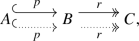
A double (short) exact sequence in ${\mathsf {C}}$ is the datum of two short exact sequences

$$\begin{aligned} \mathrm {Yin}:A\overset{p}{\hookrightarrow }B\overset{r}{\twoheadrightarrow }C\qquad \text {and}\qquad \mathrm {Yang}:A\overset{q}{\hookrightarrow } B\overset{s}{\twoheadrightarrow }C\text {,} \end{aligned}$$

where only the maps may differ, but the objects agree for both the Yin and Yang exact sequence. We write

(3.4)

as a shorthand.

The same concept would also be called a binary exact sequence when following the conventions à la Grayson [13, 15, 17].

Theorem 3.1

Let ${\mathsf {C}}$ be an exact category. Then the abelian group $K_{1}({\mathsf {C}})$ has the following presentation:

• 1. We attach a generator to each double exact sequence

  

  where A, B and C are objects in ${\mathsf {C}}$.

• 2. Whenever the Yin and Yang exact sequences agree, i.e.,

  

  (3.5)

  we declare the class to vanish.

• 3. Suppose there is a (not necessarily commutative) $(3\times 3)$-diagram

  

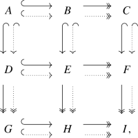
  whose rows $Row_{i}$ and columns $Col_{j}$ are double exact sequences. Suppose after deleting all Yin (resp. all Yang) exact sequences, the remaining diagram commutes. Then we impose the relation

  $$\begin{aligned} Row_{1}-Row_{2}+Row_{3}=Col_{1}-Col_{2}+Col_{3}\text {.} \end{aligned}$$

  (3.6)

Remark 3.2

(Compatibility with literature) Our notational convention regarding whether the Yin or Yang arrow is depicted top is opposite to the one used in Nenashev’s papers [19,20,21], and closer to the ordering used in Weibel’s K-theory book, e.g., in the example [26, Chapter IV, Example 9.6.2]. Our top arrow corresponds to Weibel’s left arrow. In particular, if $\varphi :X\rightarrow X$ is an automorphism of an object in an exact category ${\mathsf {C}}$, the standard map $\text {Aut}(X)\rightarrow K_{1}({\mathsf {C}})$ maps it to

See [21, Eq. 2.2] for a discussion of this. This is the map which in the special case of ${\mathsf {C}}$ being the exact category of finitely generated projective R-modules over some ring R amounts to sending an automorphism to its matrix in ${\text {GL}}(R)/[{\text {GL}} (R),{\text {GL}}(R)]=:K_{1}(R)=K_{1}({\mathsf {C}})$. Further, the vertex $(P,P^{\prime })$ in the Gillet–Grayson model lies in the connected component of $[P^{\prime }]-[P]\in \pi _{0}K({\mathsf {C}})$, i.e., also precisely opposite to Nenashev’s conventions, cf. [24, Sect. 1, middle of p. 176]. In order to be particularly sure about which arrows belong to the Yin or Yang side, we do not only distinguish by top/bottom or left/right arrows, but also use solid versus dotted arrows. If one were to use the opposite convention, i.e., interchanging Yin and Yang sequences, this amounts to an overall change of signs, but nothing more.

In fact, we shall only need the relations coming from $(3\times 3)$-diagrams in two special instances, which are worth being spelled out explicitly.

Definition 3.1

When we are given a $(3\times 3)$-diagram of the shape

satisfying the assumptions of Theorem 3.1.(3), we call

$$\begin{aligned} Row_{1}\hookrightarrow Row_{2}\twoheadrightarrow Row_{3} \end{aligned}$$

a short exact sequence of double exact sequences.

In the framework of [13] and [15] this amounts to the genuine concept of exact sequences in the exact category of (support-bounded) binary complexes. The above formulation is modelled to stress the interplay with the $(3\times 3)$-diagram relations.

Lemma 3.1

Suppose we are given a short exact sequence as in the above definition. Then the relation

$$\begin{aligned} Row_{1}-Row_{2}+Row_{3}=0 \end{aligned}$$

holds in $K_{1}({\mathsf {C}})$.

Proof

This is directly implied by the relation of the shown $(3\times 3)$-diagram since $Col_{i}=0$ for $i=1,2,3$ as the Yin and Yang sides of the columns agree (using the relation of Eq. (3.5)). $\square$

Lemma 3.2

For a $(3\times 3)$-diagram of the shape

we obtain the relation

Proof

Immediate. $\square$

There is also a deeper reason why the above special cases are sufficient: The paper [15] shows that the $K_{1}$-group has an alternative presentation, where one also uses all double exact sequences as generators, but replaces the relations coming from $(3\times 3)$-diagrams by the relations of the types appearing in Lemma 3.1 and Lemma 3.2.

Lemma 3.3

We have .

Proof

By Remark 3.2 the left term agrees with $\tilde{l}(\varphi )$ in [21, Eq. 2.2], and thus with $l(\varphi )$ by Lemma 3.1, loc. cit. Translating back with Remark 3.2 yields our claim. $\square$

4 The comparison map

Suppose ${\mathfrak {A}}$ is an arbitrary order in a finite-dimensional semisimple ${\mathbb {Q}}$-algebra A. In this section we shall set up a concrete map from the Bass–Swan presentation of $K_{0}({\mathfrak {A}} ,{\mathbb {R}})$ to the Nenashev presentation of $K_{1}(\mathsf {LCA} _{{\mathfrak {A}}})$.

We recall: If P denotes a finitely generated projective right ${\mathfrak {A}}$-module, we write $P_{{\mathbb {R}}}$ to denote the base change $P\otimes _{{\mathfrak {A}}}A_{{\mathbb {R}}}$. For every such P, we have a canonical short exact sequence

$$\begin{aligned} P\overset{\iota _{P}}{\hookrightarrow }P_{{\mathbb {R}}}\overset{q_{P} }{\twoheadrightarrow }T_{P}\qquad \text {in}\qquad \mathsf {LCA}_{{\mathfrak {A}} }\text {,} \end{aligned}$$

(4.1)

where P refers to itself, equipped with the discrete topology, $P_{{\mathbb {R}}}$ is equipped with the real vector space topology, and $T_{P}$ denotes the quotient taken in $\mathsf {LCA}_{{\mathfrak {A}}}$. This means that the underlying topological space of $T_{P}$ is a real torus ${\mathbb {T}}^{n}$ with $n:=\dim _{{\mathbb {R}}}(P_{{\mathbb {R}}})$. The key point is that, topologically, P is a discrete full rank lattice in $P_{{\mathbb {R}}}$.

Now consider a generator $[P,\varphi ,Q]$ in the Bass–Swan presentation. Then $\varphi :P_{{\mathbb {R}}}\overset{\sim }{\rightarrow }Q_{{\mathbb {R}}}$ is an isomorphism. Note that alongside

$$\begin{aligned} Q\overset{\iota _{Q}}{\hookrightarrow }Q_{{\mathbb {R}}}\overset{q_{Q} }{\twoheadrightarrow }T_{Q} \end{aligned}$$

(4.2)

we also get the short exact sequence

$$\begin{aligned} Q\overset{\varphi ^{-1}\circ \iota _{Q}}{\hookrightarrow }P_{{\mathbb {R}}} \overset{q_{Q}\circ \varphi }{\twoheadrightarrow }T_{Q}\text {.} \end{aligned}$$

(4.3)

It is basically the same, but we have replaced the middle object via the isomorphism $\varphi$. This sequence will henceforth play an important role.

We now make the following crucial definition (and explain some potentially unclear notation below the definition):

Definition 4.1

Let $(P,\varphi ,Q)$ be an object in the category $\mathsf {Sw}({\mathfrak {A}} ,A_{{\mathbb {R}}})$. We write $\left\langle \left\langle P,\varphi ,Q\right\rangle \right\rangle$ for the double exact sequence

which arises as follows:

(4.4)

In the above figure, the three columns correspond to the left, middle and right object in the double exact sequence. The corresponding left (resp. middle, resp. right) object in the double exact sequence arises by taking the direct sum of the left (resp. middle, resp. right) column. The solid arrows correspond to the Yin arrows, the dotted ones to Yang. We have used some shorthands here, which we explain now:

• 1. The symbol $\bigoplus P$ refers to the coproduct indexed over ${\mathbb {Z}}_{\ge 0}$. By the map “s” (as in ‘shift’) in $P\hookrightarrow \bigoplus P\overset{s}{\twoheadrightarrow }\bigoplus P$ we mean the map

  $$\begin{aligned} (p_{0},p_{1},p_{2},\ldots )\mapsto (p_{1},p_{2},\ldots )\text {.} \end{aligned}$$

  (4.5)

  Analogously, for Q.

• 2. The symbol $\prod T_{P}$ refers to the product indexed over ${\mathbb {Z}}_{\ge 0}$. By the map “s” (again as in ‘shift’) in $\prod T_{P}\overset{s}{\hookrightarrow }\prod T_{P}\twoheadrightarrow T_{P}$ we mean the map

  $$\begin{aligned} (t_{0},t_{1},t_{2},\ldots )\mapsto (0,t_{0},t_{1},\ldots )\text {.} \end{aligned}$$

We note that $\bigoplus P$ carries the discrete topology, and $\prod T_{P}$ is compact by Tychonoff’s theorem. To make it more readable, we have neglected labeling the arrows in the cases where it is clear: among the $\bigoplus P$ and $\prod T_{P}$, resp. for Q, the horizontal exact sequences stem from the shift maps s, and their kernels resp. cokernels. The single arrows “1”  are identity maps.

Remark 4.1

We call both shift maps s, although in reality they are different. Since it is always apparent from the context which one to use (e.g., whether we talk about discrete modules or tori), this should rather be a simplification of the notation than introduce a huge risk of confusion.

Theorem 4.1

Suppose ${\mathfrak {A}}$ is an arbitrary order in a finite-dimensional semisimple ${\mathbb {Q}}$-algebra A. The map

$$\begin{aligned} \vartheta :K_{0}({\mathfrak {A}},{\mathbb {R}})&\longrightarrow K_{1} (\mathsf {LCA}_{{\mathfrak {A}}})\\ [P,\varphi ,Q]&\longmapsto \left\langle \left\langle P,\varphi ,Q\right\rangle \right\rangle \end{aligned}$$

is well-defined.

We shall split the slightly involved proof into several lemmata, whose combination settles the claim.

Lemma 4.1

For any short exact sequence

$$\begin{aligned} (P^{\prime },\varphi ^{\prime },Q^{\prime })\overset{a}{\longrightarrow } (P,\varphi ,Q)\overset{b}{\longrightarrow }(P^{\prime \prime },\varphi ^{\prime \prime },Q^{\prime \prime }) \end{aligned}$$

as in Relation A (Eq. 3.2), we have

$$\begin{aligned}{}[\left\langle \left\langle P,\varphi ,Q\right\rangle \right\rangle ]=[\left\langle \left\langle P^{\prime },\varphi ^{\prime },Q^{\prime }\right\rangle \right\rangle ]+[\left\langle \left\langle P^{\prime \prime },\varphi ^{\prime \prime },Q^{\prime \prime }\right\rangle \right\rangle ]\text {.} \end{aligned}$$

(4.6)

Proof

First of all, we note that the input datum gives rise to a commutative diagram of the shape

(4.7)

We observe that the exactness of $P^{\prime }\hookrightarrow P\twoheadrightarrow P^{\prime \prime }$ also gives natural exact sequences

$$\begin{aligned} \bigoplus P^{\prime }\hookrightarrow \bigoplus P\twoheadrightarrow \bigoplus P^{\prime \prime }\text {,}\qquad \text {and}\qquad \prod T_{P^{\prime } }\hookrightarrow \prod T_{P}\twoheadrightarrow \prod T_{P^{\prime \prime } }\text {.} \end{aligned}$$

(4.8)

The same is true for Q, $Q_{{\mathbb {R}}}$, $\bigoplus Q$, $\prod T_{Q}$. This means that we get short exact sequences for all the entries in $\left\langle \left\langle P,\varphi ,Q\right\rangle \right\rangle$, having their counterparts in $\left\langle \left\langle P^{\prime },\varphi ^{\prime },Q^{\prime }\right\rangle \right\rangle$ and $\left\langle \left\langle P^{\prime \prime },\varphi ^{\prime \prime },Q^{\prime \prime }\right\rangle \right\rangle$ on the left resp. right side. We claim that this even yields a short exact sequence of double exact sequences

$$\begin{aligned} \left\langle \left\langle P^{\prime },\varphi ^{\prime },Q^{\prime }\right\rangle \right\rangle \hookrightarrow \left\langle \left\langle P,\varphi ,Q\right\rangle \right\rangle \twoheadrightarrow \left\langle \left\langle P^{\prime \prime },\varphi ^{\prime \prime },Q^{\prime \prime }\right\rangle \right\rangle \end{aligned}$$

(4.9)

in the sense of Definition 3.1. We need to make sure that the relevant squares underlying this definition commute. This is clear for most terms. The only potentially delicate piece is the middle cross for all three terms of the exact sequences (by middle cross we mean the four diagonal arrows in formula 4.4). We just discuss the monic piece around the ‘$\hookrightarrow$’ in detail, i.e., $\left\langle \left\langle P^{\prime },\varphi ^{\prime },Q^{\prime }\right\rangle \right\rangle \hookrightarrow \left\langle \left\langle P,\varphi ,Q\right\rangle \right\rangle$; the epic piece can be treated analogously. We depict the situation below.

(4.10)

On the Yin side (the solid arrows), we just use the natural maps coming from Eq. (4.2), e.g.,

$$\begin{aligned} P^{\prime }\hookrightarrow P_{{\mathbb {R}}}^{\prime }\twoheadrightarrow T_{P^{\prime }} \end{aligned}$$

on the left. On the Yang side, we could do the same if we had $Q_{{\mathbb {R}}}$ sitting in the middle, since we have a corresponding natural sequence

$$\begin{aligned} Q^{\prime }\hookrightarrow Q_{{\mathbb {R}}}^{\prime }\twoheadrightarrow T_{Q^{\prime }}\text {.} \end{aligned}$$

Thus, we play the trick of Eq. (4.3), that is: We pre- and post-compose $Q_{{\mathbb {R}}}^{\prime }$ with the isomorphisms $\varphi ^{\prime }$, $\varphi ^{\prime -1}$; and correspondingly for $Q_{{\mathbb {R}}}$ with $\varphi ,\varphi ^{-1}$. The necessary diagram of commutativities to check that this compatibly fills the squares in formula 4.10 is precisely the diagram in Eq. (4.7). In the figure above, the front dashed contour parallelogram (the one more to the right) corresponds precisely to the left commuting square in Eq. (4.7), composed with the natural maps $q_{Q^{\prime }}$ resp. $q_{Q}$. The back dashed contour parallelogram (the one more to the left) corresponds to the same square, but for the inverse morphisms $\varphi ^{\prime -1}$ and $\varphi ^{-1}$ instead, this time pre-composed with the natural maps $\iota _{Q^{\prime }}$ resp. $\iota _{Q}$. Now apply Lemma 3.1 to Eq. (4.9), proving our claim. $\square$

Definition 4.2

Let $X\in \mathsf {LCA}_{{\mathfrak {A}}}$ be any object. We define

(4.11)

where q swaps both summands, i.e., $(x,y)\mapsto (y,x)$.

Relation B (Eq. 3.3) is a little more complicated to handle. It is already not completely obvious that $[P,\text {id},P]$ is being sent to zero. Hence, as a warm-up and illustration of the general method, let us prove this first.

Lemma 4.2

The map $\vartheta$ sends $[P,\text {id},P]$ to zero.

Proof

Unravelling definitions, we find that $\left\langle \left\langle P,\text {id},P\right\rangle \right\rangle$ corresponds to the double exact sequence depicted below on the left:

(4.12)

Next, we produce a morphism of double exact sequences from the left to the right. Objectwise, the maps are: (a) the identity on the Yin side everywhere, (b) and on the Yang side, we use the swap map

$$\begin{aligned} \prod T_{P}\oplus \prod T_{P}&\longrightarrow \prod T_{P}\oplus \prod T_{P}\nonumber \\ (x,y)&\longmapsto (y,x) \end{aligned}$$

(4.13)

and analogously we swap the summands of $P\oplus P$, as well as of $\bigoplus P\oplus \bigoplus P$. We use the identity map on $P_{{\mathbb {R}}}$. Let us explain this along formula 4.12: One can think about the map which we have just described in two ways: Firstly, as exchanging all objects $\prod T_{P}$, P,  $\bigoplus P$ on the upper half of the figure with their counterparts on the lower half; the object $P_{{\mathbb {R}}}$ remains where it is. When we speak of the top and lower half here, we do not mean the Yin and Yang side, but we rather just mean the obvious symmetry of formula 4.12 when mirroring it along the horizontal middle axis. Our swapping operation only refers to this symmetry and only to the Yang side, i.e., the dotted arrows. However, in the above figure on the right, we use a different graphical presentation: Instead of swapping the objects, we leave all the objects at precisely the same position as before. Instead, we swap all the dotted (i.e., Yang) arrows between them. So, one way to think about going from left to right is that all the dotted arrows $(A)\dashrightarrow (B)$ on the upper half get exchanged with their corresponding arrow $(A)\dashrightarrow (B)$ on the lower half. In total, we are in the situation of Lemma 3.2, mapping through a number of swaps $\sigma _{(\ldots )}$ from $\left\langle \left\langle P,\text {id},P\right\rangle \right\rangle$ to S, where S denotes the double exact sequence on the right in formula 4.12. Precisely, the relevant arrows are those induced from $\text {id}:P_{{\mathbb {R}}}\rightarrow P_{{\mathbb {R}}}$ (for both Yin and Yang), the identity on all objects on the Yin side, and the swapping maps of Eq. (4.13) for all other objects on the Yang side. Lemma 3.2 thus yields

$$\begin{aligned}{}[\left\langle \left\langle P,\text {id},P\right\rangle \right\rangle ]-[S]&=\sigma _{ {\textstyle \prod } T_{P}}+\sigma _{P}-\sigma _{ {\textstyle \prod } T_{P}}-\sigma _{ {\textstyle \bigoplus } P}+\sigma _{T_{P}}+\sigma _{ {\textstyle \bigoplus } P}\\&=\sigma _{P}+\sigma _{T_{P}}\text {.} \end{aligned}$$

However, $\sigma _{P}=0$ because the exact sequence $P\hookrightarrow {\textstyle \bigoplus } P\overset{s}{\twoheadrightarrow } {\textstyle \bigoplus } P$ of the shift map gives rise to a short exact sequence of double exact sequences,

$$\begin{aligned} \sigma _{P}\hookrightarrow \sigma _{ {\textstyle \bigoplus } P}\twoheadrightarrow \sigma _{ {\textstyle \bigoplus } P} \end{aligned}$$

and by Lemma 3.1 this implies $\sigma _{P}-\sigma _{ {\textstyle \bigoplus } P}+\sigma _{ {\textstyle \bigoplus } P}=0$. Using the shift exact sequence for $T_{P}$, we also get $\sigma _{T_{P} }=0$. Hence, $[\left\langle \left\langle P,\text {id},P\right\rangle \right\rangle ]=[S]$, but $[S]=0$ since the Yin and Yang sides agree. $\square$

With this preparation, we are ready for a generalization of the previous lemma.

Lemma 4.3

The map $\vartheta$ respects Relation B (Eq. (3.3)), i.e., we have

$$\begin{aligned}{}[\left\langle \left\langle P,\psi \varphi ,R\right\rangle \right\rangle ]=[\left\langle \left\langle P,\varphi ,Q\right\rangle \right\rangle ]+[\left\langle \left\langle Q,\psi ,R\right\rangle \right\rangle ] \end{aligned}$$

for arbitrary $(P,\varphi ,Q)$ and $(Q,\psi ,R)$.

Proof

We consider the sum $\left\langle \left\langle P,\varphi ,Q\right\rangle \right\rangle +\left\langle \left\langle Q,\psi ,R\right\rangle \right\rangle$, which agrees with the class of

$$\begin{aligned} J:=\left\langle \left\langle P\oplus Q,\varphi \oplus \psi ,Q\oplus R\right\rangle \right\rangle \end{aligned}$$

by using the direct sum split exact sequence and Lemma 3.1. The latter double exact sequence can be depicted as follows below on the left:

(4.14)

and we ignore the shaded areas for the moment. We now set up maps from J to a new double exact sequence: The idea is that we map the double exact sequence to itself, just that on the objects $T_{Q},\prod T_{Q},Q,\bigoplus Q$, which each appear twice in the shaded areas, we use the identity map on the Yin side, but swap both objects on the Yang side. On $P_{{\mathbb {R}}}$ and $Q_{{\mathbb {R}}}$ we use the identity both for Yin and Yang. We call this output $J^{\prime }$. It is depicted in formula 4.14 above on the right. As before in the proof of Lemma 4.2, in this figure we have left all objects where they were and just adjusted the arrows. The solid arrows, i.e., the Yin side, of J and $J^{\prime }$ agree, but we see that on the Yang side all arrows have moved to their respective mirror partner. These maps serve as input for Lemma 3.2, giving the relation

$$\begin{aligned}{}[J]-[J^{\prime }]&=\sigma _{Q}+\sigma _{ {\textstyle \prod } T_{Q}}-\sigma _{ {\textstyle \bigoplus } Q}-\sigma _{ {\textstyle \prod } T_{Q}}+\sigma _{ {\textstyle \bigoplus } Q}+\sigma _{T_{Q}}\nonumber \\&=\sigma _{Q}+\sigma _{T_{Q}}=0\text {,} \end{aligned}$$

(4.15)

because the latter classes $\sigma _{Q},\sigma _{T_{Q}}$ both vanish by the same argument as in the proof of Lemma 4.2. Next, within the shaded area of formula 4.14 on the right, we find the doubled versions of the same exact sequences

$$\begin{aligned}&\prod T_{Q}\overset{s}{\hookrightarrow }\prod T_{Q}\twoheadrightarrow T_{Q}\qquad \text {and}\qquad \prod T_{Q}\overset{1}{\hookrightarrow }\prod T_{Q}\twoheadrightarrow 0\text {,} \\&Q\hookrightarrow \bigoplus Q\overset{s}{\twoheadrightarrow }\bigoplus Q\qquad \text {and}\qquad 0\hookrightarrow \bigoplus Q\overset{1}{\twoheadrightarrow }\bigoplus Q\text {.} \end{aligned}$$

For these both Yin and Yang morphisms agree. We can map them as a sub-double exact sequence to $J^{\prime }$, giving rise to a short exact sequence of double exact sequences, but since Yin and Yang agree, they all contribute the zero class. Thus, the class of $[J^{\prime }]$ agrees with its quotient by these sequences (by Lemma 3.1), which yields the double exact sequence depicted below on the left:

We now map the double exact sequence on the left to the one depicted above on the right. To this end, we use identity maps on all objects except for $Q_{{\mathbb {R}}}$, where we instead use $\varphi ^{-1}$ both for Yin and Yang (as alluded to by the dashed arrow in the figure). As the reader can see, we have adjusted the maps on the right hand side to ensure that this defines a commuting diagram (obviously it suffices to change the four in- resp. out-going maps around $Q_{{\mathbb {R}}}$ resp. $P_{{\mathbb {R}}}$ to accomodate for these changes). Write $J^{\prime \prime }$ for the double exact sequence on the right. The morphism just described again has the format suitable for using Lemma 3.2, this time showing $[J^{\prime }]-[J^{\prime \prime }]=0-0+0$. There are only zeros on the right-hand side since we only use the identity map, or $(\varphi ^{-1},\varphi ^{-1})$ for both Yin and Yang, which is zero by Eq. (3.5). Finally, we set up a map from $J^{\prime \prime }$ (above on the right) to $J^{\prime \prime \prime }$, defined as

This map is the identity on all objects on the Yin side. On the Yang side, it is the identity on all objects, except on the pair $P_{{\mathbb {R}}}\oplus P_{{\mathbb {R}}}$, on which it swaps the two direct summands. The morphism again can serve as input for Lemma 3.2. It yields the relation

$$\begin{aligned}{}[J^{\prime \prime }]-[J^{\prime \prime \prime }]=-\sigma _{P_{{\mathbb {R}}}} \end{aligned}$$

in the notation of Eq. (4.11). From Sequence 4.1 we get a short exact sequence of double exact sequences showing $\sigma _{P_{{\mathbb {R}} }}=\sigma _{P}+\sigma _{T_{P}}$ and the latter two classes vanish by the same argument as in Eq. (4.15). Just as we had killed the pieces in the shaded areas in formula 4.14, we can now get rid of the doubled exact sequence $Q\hookrightarrow P_{{\mathbb {R}}}\twoheadrightarrow T_{Q}$ in the middle, where the Yin and Yang side agree. The resulting double exact sequence is exactly $\left\langle \left\langle P,\psi \varphi ,R\right\rangle \right\rangle$. Thus, using that we had shown that $[J]=[J^{\prime }]=[J^{\prime \prime }]=[J^{\prime \prime \prime }]$, we deduce

$$\begin{aligned}{}[\left\langle \left\langle P,\varphi ,Q\right\rangle \right\rangle ]-[\left\langle \left\langle P,\psi \varphi ,R\right\rangle \right\rangle ]+[\left\langle \left\langle Q,\psi ,R\right\rangle \right\rangle ]=0\text {,} \end{aligned}$$

which proves that Relation B is respected under our map $\vartheta$. $\square$

5 The map is an isomorphism

5.1 Recollections on the Gillet–Grayson model

Let ${\mathsf {C}}$ be a pointed exact category, i.e., an exact category with a fixed choice of a zero object which we shall henceforth denote by “0”. We briefly summarize the Gillet–Grayson model. It originates from the articles [11, 12]. Define a simplicial set $G_{\bullet }{\mathsf {C}}$ whose n-simplices are given by a pair of commutative diagrams

such that (1) the diagrams agree strictly above the bottom row, (2) all sequences $P_{i}\hookrightarrow P_{j}\twoheadrightarrow P_{j/i}$ are exact, (2’) all sequences $P_{i}^{\prime }\hookrightarrow P_{j}^{\prime } \twoheadrightarrow P_{j/i}^{\prime }$ are exact, (3) all sequences $P_{i/j}\hookrightarrow P_{m/j}\twoheadrightarrow P_{m/i}$ are exact.

The face and degeneracy maps come from deleting the i-th row and column, or by duplicating them. For details we refer to the references. As we can see from the above description, the 0-simplices are pairs $(P,P^{\prime })$ of objects. The 1-simplices are pairs of exact sequences

(5.1)

with the same cokernel. The main result of Gillet and Grayson is the equivalence

$$\begin{aligned} K({\mathsf {C}})\cong \left| G_{\bullet }{\mathsf {C}}\right| \text {,} \end{aligned}$$

or more specifically: The space $\left| G_{\bullet }{\mathsf {C}}\right|$ carries an infinite loop space structure and as such is equivalent to a connective spectrum. This spectrum is canonically equivalent to the K-theory spectrum of ${\mathsf {C}}$. As explained in Remark 3.2, the 0-simplex $(P,P^{\prime })$ lies in the connected component $[P^{\prime }]-[P]\in \pi _{0}K({\mathsf {C}})$.

Definition 5.1

(Nenashev) If $A\in {\mathsf {C}}$ is an object, let e(A) denote the edge

from (0, 0) to (A, A). To any double exact sequence $\kappa$ in ${\mathsf {C}}$, we now attach a loop $e(\kappa )\in \pi _{1}K({\mathsf {C}})$. Concretely,

is mapped to a path made from three 1-simplices in the Gillet–Grayson model, namely

• 1. we go from (0, 0) to (A, A) by the edge e(A),

• 2. then we go from (A, A) to (B, B) by the edge

  

• 3. and then we return from (B, B) to (0, 0) by running backwards along e(B).

The path $e(\kappa )$ is visibly a closed loop. All vertices lie in the connected component of zero in $\left| G_{\bullet }{\mathsf {C}}\right|$. This construction agrees with the $e(\kappa )$ in [21, Eq. 2.2 $\frac{1}{2}$], except for the swapped roles of left and right, in line with Remark 3.2.

5.2 Proof

Theorem 5.1

Suppose ${\mathfrak {A}}$ is a regular order in a semisimple finite-dimensional ${\mathbb {Q}}$-algebra A. Then the diagram

(5.2)

commutes up to signs ($-1$ for the square X, $+1$ for the square Y), where (1) $\delta$ is the connecting map in the relative K-theory sequence of Bass–Swan, (2) $\partial$ is the connecting map in the long exact sequence as constructed in [5, Theorem 11.3], (3) $\vartheta$ is the map of Theorem 4.1. In particular, the map $\vartheta$ is an isomorphism.

We split the proof into several lemmata.

Lemma 5.1

The square denoted by X in Eq. (5.2) commutes up to the constant sign $-1$.

Proof

Let an element in $K_{1}(A_{{\mathbb {R}}})$ be given, say represented by some matrix $\varphi \in {\text {GL}}_{n}(A_{{\mathbb {R}}})$ for n sufficiently large. We follow the downward and then right arrow first: The downward arrow is the identity. The bottom map is induced from the exact functor $\text {PMod}(A_{{\mathbb {R}}})\rightarrow \mathsf {LCA}_{{\mathfrak {A}}}$ which sends a finitely generated projective right $A_{{\mathbb {R}}}$-module to itself, regarded as a locally compact module with the real topology (since $A_{{\mathbb {R}}}$ is semisimple, finitely generated projective just means free of finite rank here). The image of the class represented by $\varphi$ still corresponds to an automorphism, now of the locally compact module, and by Remark 3.2 it has the Nenashev representative

(5.3)

Next, follow the square the other way: Following the top right arrow, we get

$$\begin{aligned} \delta (\varphi )=[{\mathfrak {A}}^{n},\varphi ,{\mathfrak {A}}^{n}]\in K_{0} ({\mathfrak {A}},{\mathbb {R}})\text {,} \end{aligned}$$

using the explicit presentation, see [25, p. 215] or [26, Chapter II, Definition 2.10 and Exercise 2.17]. The map $\vartheta$ sends this to the class of $\left\langle \left\langle {\mathfrak {A}}^{n} ,\varphi ,{\mathfrak {A}}^{n}\right\rangle \right\rangle$, which in turn unravels as the double exact sequence depicted below on the left:

We now show that its class agrees with the class of the double exact sequence depicted above on the right. The proof for this follows exactly the same pattern as the proof of Lemma 4.2 and we leave the details to the reader. However, unlike in the cited proof, this time the middle double exact sequence (the one which is bent in the figure above on the right) can be non-trivial. We use it as the first row in the following $(3\times 3)$-diagram:

That is: it becomes an instance of Lemma 3.2. Using that the top row of this diagram represents the class of $\left\langle \left\langle {\mathfrak {A}}^{n},\varphi ,{\mathfrak {A}}^{n}\right\rangle \right\rangle$ as we had just shown, the resulting relation reads

but this agrees with Eq. (5.3) up to the sign $-1$ by Lemma 3.3. $\square$

We recall the following definition since it plays a fairly important role in the next proof.

Definition 5.2

Suppose $G\in \mathsf {LCA}$. A subset $U\subseteq G$ is called symmetric if $g\in U$ implies $-g\in U$. The group G is called compactly generated¹ if there exists a symmetric compact subset $C\subseteq G$ such that $G=\bigcup _{n\ge 0}C^{n}$, where $C^{n}=\{c_{1}+\cdots +c_{n}\mid c_{i}\in C\}$. We write $\mathsf {LCA}_{{\mathfrak {A}},cg}$ for the fully exact subcategory of those objects in $\mathsf {LCA}_{{\mathfrak {A}}}$ whose underlying LCA group is compactly generated.

Lemma 5.2

The square denoted by Y in Eq. (5.2) commutes.

Proof

Let $[P,\varphi ,Q]\in K_{0}({\mathfrak {A}},{\mathbb {R}})$ be an arbitrary element. Then under the top right arrow it is sent to

$$\begin{aligned}{}[P]-[Q]\in K_{0}({\mathfrak {A}})\text {,} \end{aligned}$$

(5.4)

see [25, p. 215] or [26, Chapter II, Definition 2.10]. Thus, it remains to see that we also get this if we follow the square the other way: Firstly, the map $\vartheta$ sends $[P,\varphi ,Q]$ to the class of the double exact sequence $\left\langle \left\langle P,\varphi ,Q\right\rangle \right\rangle$, i.e.,

(5.5)

Thus, we need to compute what the map $\partial$ in Diagram 5.2 does with this element. We begin by describing how the connecting map

$$\begin{aligned} \partial :K_{1}(\mathsf {LCA}_{{\mathfrak {A}}})\longrightarrow K_{0} ({\mathfrak {A}}) \end{aligned}$$

arises in [5]. This leads us to the proof of [5, Proposition 11.1]. In this proof, we first set up the diagram

where $\mathsf {Mod}_{{\mathfrak {A}},fg}$ denotes the category of finitely generated right ${\mathfrak {A}}$-modules, $\mathsf {Mod}_{{\mathfrak {A}}}$ the category of all right ${\mathfrak {A}}$-modules, and $\mathsf {LCA}_{{\mathfrak {A}} ,cg}=\mathsf {LCA}_{{\mathfrak {A}}}\cap \mathsf {LCA}_{cg}$ as in Definition 5.2. Both rows stem from Schlichting’s construction of quotient exact categories [22, Proposition 1.16], which generalizes the construction of quotients of abelian categories by Serre subcategories to the setting of exact categories. These rows are exact sequences of exact categories (in the sense that the induced sequence between their bounded derived categories $D^{b}(-)$ is a Verdier localization sequence, [22, Proposition 2.6]). The middle downward arrow sends a right ${\mathfrak {A}}$-module to itself, equipped with the discrete topology. The other downward arrows are compatibly induced from this. In the proof of [5, Proposition 11.1] it is shown that $\Phi$ is in fact an exact equivalence of exact categories. In particular, it induces an equivalence on the level of non-connective K-theory. Applying non-connective K-theory to the entire diagram, we get two fiber sequences and a map between these fiber sequences which induces an equivalence on the cofiber. It follows that the left square is bi-Cartesian in spectra. The lower long exact sequence in Diagram 5.2 now is taken to be the long exact sequence of (stable) homotopy groups arising from this, using that the bi-Cartesian diagram has a contractible node. From this, one unravels by diagram chase that the differential

$$\begin{aligned} \partial :\pi _{1}K(\mathsf {LCA}_{{\mathfrak {A}}})\longrightarrow \pi _{0}K\mathbb {(}\mathsf {Mod}_{{\mathfrak {A}},fg}) \end{aligned}$$

agrees with the composition $\partial ^{*}\circ \Phi ^{-1}\circ q$ in the following diagram

where $\partial ^{*}$ is the connecting map of the long exact sequence of homotopy groups coming from the fiber sequence in the top row, i.e., coming from

$$\begin{aligned} \mathsf {Mod}_{{\mathfrak {A}},fg}\longrightarrow \mathsf {Mod}_{{\mathfrak {A}} }\longrightarrow \mathsf {Mod}_{{\mathfrak {A}}}/\mathsf {Mod}_{{\mathfrak {A}} ,fg}\text {.} \end{aligned}$$

Several further remarks: The proof of [5, Theorem 11.3] shows that the non-connective K-theory of all the involved categories agrees with their connective K-theory, i.e., their usual Quillen algebraic K-theory. Thus, from now on view $K(-)$ as a connective spectrum. We now unravel the maps in $\partial ^{*}\circ \Phi ^{-1}\circ q$:(Step 1) The map q is induced from the exact quotient functor

$$\begin{aligned} \mathsf {LCA}_{{\mathfrak {A}}}\longrightarrow \mathsf {LCA}_{{\mathfrak {A}} }/\mathsf {LCA}_{{\mathfrak {A}},cg}\text {.} \end{aligned}$$

Thus, q sends the double exact sequence in formula 5.5 to itself, but regarded as an object in $\mathsf {LCA}_{{\mathfrak {A}}}/\mathsf {LCA} _{{\mathfrak {A}},cg}$ now. We observe that P is finitely generated projective and thus has underlying LCA group isomorphic to ${\mathbb {Z}}^{n}$ for some $n\in {\mathbb {Z}}_{\ge 0}$. Since $T_{P}$ is a torus, it is compact, and by Tychonoff’s Theorem, $\prod T_{P}$ is also compact. Both arguments also work verbatim for Q and $\prod T_{Q}$. Further, the underlying LCA group of $P_{{\mathbb {R}}}$ is a finite-dimensional real vector space. Thus, by the classification of compactly generated LCA groups, all these objects are compactly generated, see [18, Theorem 2.5]. As a result, for each such object we obtain an isomorphism to the zero object in the category $\mathsf {LCA}_{{\mathfrak {A}}}/\mathsf {LCA}_{{\mathfrak {A}},cg}$. Thus, the class of $q(\left\langle \left\langle P,\varphi ,Q\right\rangle \right\rangle )$ is given by the double exact sequence l, defined as

(5.6)

We recall that s is the shift map of Eq. (4.5). It may appear like a mistake that the shift maps s are both depicted with kernel “0”, but this is accurate since while in the category $\mathsf {LCA}_{{\mathfrak {A}}}$ the kernel would be P resp. Q, in the quotient category $\mathsf {LCA}_{{\mathfrak {A}}}/\mathsf {LCA} _{{\mathfrak {A}},cg}$ these objects are isomorphic to zero. Next, we need to apply the map $\Phi ^{-1}$. Being the inverse map to a functor, this is usually a tough operation, but it is easy in our situation: Note that all objects in formula 5.6 are discrete right ${\mathfrak {A}}$-modules, so we can right away read this as a double exact sequence in $\mathsf {Mod} _{{\mathfrak {A}}}/\mathsf {Mod}_{{\mathfrak {A}},fg}$, which $\Phi$ obviously sends to itself. Finally, we need to apply $\partial ^{*}$. This is more delicate: Recall that

$$\begin{aligned} K\mathbb {(}\mathsf {Mod}_{{\mathfrak {A}},fg})\longrightarrow K(\mathsf {Mod} _{{\mathfrak {A}}})\longrightarrow K\mathbb {(}\mathsf {Mod}_{{\mathfrak {A}} }/\mathsf {Mod}_{{\mathfrak {A}},fg}) \end{aligned}$$

(5.7)

is a fiber sequence in spectra coming from the Verdier localization sequence of [22, Proposition 2.6]. As all spectra here are connective, we may read this as a fiber sequence of infinite loop spaces as well. We take simplicial sets $\mathsf {sSet}$ as our $\infty$-category of ‘spaces’. Next, use Gillet–Grayson’s model $G_{\bullet }(-)$ to have a simplicial set describing K-theory; we had reviewed what we need in Sect. 5.1. Now, the connecting map

$$\begin{aligned} \partial ^{*}:\pi _{1}K(\mathsf {Mod}_{{\mathfrak {A}}}/\mathsf {Mod} _{{\mathfrak {A}},fg})\longrightarrow \pi _{0}K\mathbb {(}\mathsf {Mod} _{{\mathfrak {A}},fg}) \end{aligned}$$

(5.8)

has the following topological meaning: We will first explain this as if

$$\begin{aligned} G_{\bullet }(\mathsf {Mod}_{{\mathfrak {A}}})\longrightarrow G_{\bullet }(\mathsf {Mod}_{{\mathfrak {A}}}/\mathsf {Mod}_{{\mathfrak {A}},fg}) \end{aligned}$$

(5.9)

were a fibration of simplicial sets (which it is not, but we will fix this issue below). So assume it were. Then we take a loop $\ell$ in the space $G_{\bullet }(\mathsf {Mod}_{{\mathfrak {A}}}/\mathsf {Mod}_{{\mathfrak {A}},fg})$ and lift it along this fibration. This is possible, but only as a path which need not be closed, so we obtain a path from the distinguished point of $G_{\bullet }(\mathsf {Mod}_{{\mathfrak {A}}})$, which is the point defined by (0, 0) for the zero object in the Gillet–Grayson model, to some other point, which in concrete terms is a pair (A, B). The boundary map $\partial ^{*}$ then sends $\ell$ to the connected component in which this endpoint (A, B) lies.

As we had explained, the map in Eq. (5.9) actually fails to be a fibration. The fact that Eq. (5.7) is a fiber sequence stems from modifying a genuine fiber sequence of simplicial sets through various equivalences. Luckily, the only issue this creates for the map in Eq. (5.9) is that we possibly cannot lift an arbitrary path. However, if we can manually present a path which does lift a given path, then the rest of the computation is still valid. How to see this is explained in detail in [23, Lemma 2.1].

Thus, it remains to exhibit such a manual lift in the Gillet–Grayson model. In the case at hand, the double exact sequence $\Phi ^{-1}q(\left\langle \left\langle P,\varphi ,Q\right\rangle \right\rangle )$ is our input loop, and we had seen that the description of formula 5.6 is valid. It corresponds to the path

(5.10)

Recall that l was the double exact sequence of formula 5.6. As explained above, we now need to lift this loop to a path in the Gillet–Grayson space of $\mathsf {Mod}_{{\mathfrak {A}}}$. We recall that an edge from the point $(P_{0},P_{0}^{\prime })$ to a point $(P_{1},P_{1}^{\prime })$ in the Gillet–Grayson model corresponds to a pair of exact sequences with equal cokernels. Concretely, we shall take

(5.11)

which visibly have equal cokernels. This defines an edge. We now replace the edge f in formula 5.10 by this new edge. We get a non-closed path

(5.12)

The key point is that this path also defines a path in $G_{\bullet }(\mathsf {Mod}_{{\mathfrak {A}}})$, much unlike formula 5.10 which would not since the shift map s is not an isomorphism in the category $\mathsf {Mod}_{{\mathfrak {A}}}$. We claim that formula 5.12 serves the purpose of providing a lift of our loop: Indeed, under the map

$$\begin{aligned} G_{\bullet }(\mathsf {Mod}_{{\mathfrak {A}}})\longrightarrow G_{\bullet }(\mathsf {Mod}_{{\mathfrak {A}}}/\mathsf {Mod}_{{\mathfrak {A}},fg}) \end{aligned}$$

(5.13)

the kernels P and Q which appear on the left in Eq. (5.11) again become isomorphic to zero since they are finitely generated, and thus the upper edge transforms to f again. As we had discussed above, irrespectively of Eq. (5.13) not coming from a fibration, the boundary map $\partial ^{*}$ of Eq. (5.8) maps the lifted path to the connected component of its endpoint. This endpoint is (Q, P). However, the identification

$$\begin{aligned} \pi _{0}\left| G_{\bullet }(\mathsf {Mod}_{{\mathfrak {A}},fg})\right| \overset{\sim }{\longrightarrow }K_{0}(\mathsf {Mod}_{{\mathfrak {A}},fg}) \end{aligned}$$

in terms of the Gillet–Grayson model is given by the map $(Q,P)\mapsto [P]-[Q]$, see Remark 3.2. Finally, since ${\mathfrak {A}}$ is regular, so every finitely generated module admits a finite projective resolution, the map

$$\begin{aligned} K({\mathfrak {A}})\longrightarrow K(\mathsf {Mod}_{{\mathfrak {A}},fg}) \end{aligned}$$

induced from the functor including finitely generated projective ${\mathfrak {A}}$-modules into all finitely generated modules is an equivalence. On the level of $K_{0}$, the class $[P]-[Q]$ is just sent to itself. Hence, we have obtained the same result as in Eq. (5.4), which is exactly what we had to show. $\square$

Proof (of Theorem 5.1)

[of Theorem 5.1] Using Lemmas 5.1 and 5.2, we find that the two squares to the left as well as to the right of the downward arrow $\vartheta$ in Eq. (5.2) commute up to sign. Since all other downward arrows in these squares are isomorphisms, it follows that $\vartheta$ is an isomorphism as well by the Five Lemma. $\square$

The following remains open.

Problem 1

There should be a recipe to map a double exact sequence to a Bass–Swan generator. It should be possible to check in an elementary (but probably complicated) fashion that composing both maps either way yields the identity map.

This would in particular circumvent the simplicial arguments about lifting paths in the proof of Lemma 5.2.

Problem 2

Using the work of Grayson [13], the higher K-groups $K_{n}(\mathsf {LCA}_{{\mathfrak {A}}})$ all have explicit presentations generalizing Nenashev’s presentation for $K_{1}$. The compatibility between the Nenashev and Grayson presentations is settled first in [17], and even better in [15]. Furthermore, the long exact sequence

$$\begin{aligned} \cdots \longrightarrow K_{n}({\mathfrak {A}})\longrightarrow K_{n}(A_{{\mathbb {R}} })\longrightarrow K_{n-1}({\mathfrak {A}},{\mathbb {R}})\longrightarrow K_{n-1}({\mathfrak {A}})\longrightarrow \cdots \end{aligned}$$

involving relative K-groups can also be generalized to higher $n>0$, and the higher relative K-groups $K_{n-1}({\mathfrak {A}},{\mathbb {R}})$ admit a similar concrete model in the style of Grayson, see [14, Corollary 2.3]. Perhaps one could extend the above proof and isolate a concrete formula for the isomorphism

$$\begin{aligned} K_{n}({\mathfrak {A}},{\mathbb {R}})\overset{\sim }{\longrightarrow }K_{n+1} (\mathsf {LCA}_{{\mathfrak {A}}})\text {,} \end{aligned}$$

of Theorem 5.1 for all $n\ge 0$. It would be based on the corresponding relative versus absolute Grayson presentation using binary multi-complexes.

Problem 3

A different construction of the fiber sequence in [5] was given in [2]. Perhaps a different proof based on this new construction is simpler.

References

Burns, D., Flach, M.: Tamagawa numbers for motives with (non-commutative) coefficients. Doc. Math. 6, 501–570 (2001)
Braunling, O., Henrard, R., & van Roosmalen, A.-C.: \(K\)-theory of locally compact modules over orders. arXiv:2006.10878 [math.KT] (2020)
Bloch, S., Kato, K.: \(L\)-functions and Tamagawa numbers of motives, The Grothendieck Festschrift, Vol. I, Progr. Math., vol. 86, Birkhäuser Boston, Boston, MA, pp. 333–400 (1990)
Bloch, S.: A note on height pairings, Tamagawa numbers, and the Birch and Swinnerton-Dyer conjecture. Invent. Math. 58(1), 65–76 (1980)
Braunling, O.: On the relative \(K\)-group in the ETNC. N. Y. J. Math. 25, 1112–1177 (2019)
Braunling, O.: On the relative \(K\)-group in the ETNC, Part III. N. Y. J. Math. 26, 656–687 (2020)
Birch , B. J., Swinnerton-Dyer, H. P. F.: Notes on elliptic curves. I, J. Reine Angew. Math. 212, 7–25 (1963)
Birch, B.J., Swinnerton-Dyer, H. P. F.: Notes on elliptic curves. II, J. Reine Angew. Math. 218, 79–108 (1965)
Clausen, D.: A K-theoretic approach to Artin maps. arXiv:1703.07842 [math.KT] (2017)
Fontaine, J.-M., Perrin-Riou, B.: Autour des conjectures de Bloch et Kato: cohomologie galoisienne et valeurs de fonctions \(L\), Motives (Seattle, WA, : Proc. Sympos. Pure Math., vol. 55, Amer. Math. Soc. Providence, RI 1994, 599–706 (1991)
Gillet, H., Grayson, D.: The loop space of the \(Q\)-construction. Illinois J. Math. 31(4), 574–597 (1987)
Gillet, H., Grayson, D.: Erratum to: “The loop space of the \(Q\)-construction”. Illinois J. Math. 47(3), 745–748 (2003)
Grayson, D.: Algebraic \(K\)-theory via binary complexes. J. Am. Math. Soc. 25(4), 1149–1167 (2012)
Grayson, D.:Relative algebraic K-theory by elementary means (2016)
Kasprowski, D., Köck, B., Winges, C.: \(K_1\)-groups via binary complexes of fixed length. Homol. Homot. Appl. 22(1), 203–213 (2020)
Kottwitz, R.: Tamagawa numbers. Ann. Math. 127(2), 629–646. MR 942522 (1988)
Kasprowski, D., Winges, C.: Shortening binary complexes and commutativity of K-theory with infinite products. Trans. Am. Math. Soc. Ser. B 7, 1–23 (2020)
Moskowitz, M.: Homological algebra in locally compact abelian groups. Trans. Am. Math. Soc. 127, 361–404 (1967)
Nenashev, A., Double short exact sequences produce all elements of Quillen’s \(K_1\), Algebraic \(K\)-theory (Poznań, : Contemp. Math., vol. 199, Amer. Math. Soc. Providence, RI 1996, 151–160 (1995)
Nenashev, A.: Double short exact sequences and\(K_1\)of an exact category, \(K\)-Theory 14(1), 23–41 (1998)
Nenashev, A.: \(K_1\) by generators and relations. J. Pure Appl. Algebra 131(2), 195–212 (1998)
Schlichting, M.: Delooping the \(K\)-theory of exact categories. Topology 43(5), 1089–1103 (2004)
Sherman, C.: Group representations and algebraic \(K\)-theory, Algebraic \(K\)-theory, Part I (Oberwolfach: Lecture Notes in Math., vol. 966. Springer, Berlin 1982, 208–243 (1980)
Sherman, C.: Connecting homomorphisms in localization sequences, Algebraic \(K\)-theory (Poznań, : Contemp. Math., vol. 199, Amer. Math. Soc. Providence, RI 1996, 175–183 (1995)
Swan, R.G.: Algebraic \(K\)-theory, Lecture Notes in Mathematics, No. 76, Springer, Berlin-New York (1968)
Weibel, C.: The \(K\)-book , Graduate Studies in Mathematics, vol. 145, American Mathematical Society, Providence, RI, 2013, An introduction to algebraic \(K\)-theory
Acknowledgements
This work is heavily inspired by Dustin Clausen’s paper [9]. Bernhard Köck had concretely asked me whether the elements I discussed in my earlier papers on locally compact modules could be made explicit in the Nenashev presentation. This article provides a concrete answer. Moreover, I thank B. Chow, M. Flach, D. Grayson, A. Huber, B. Morin, A. Nickel, M. Wendt, C. Winges for discussions and/or correspondence. I thank the FRIAS, where the definition of \(\left\langle \left\langle P,\varphi ,Q\right\rangle \right\rangle \) was found, for its excellent working conditions and rich opportunities for academic exchange. I particularly thank the two anonymous referees, who both clearly read the text with great care and made a great number of insightful suggestions.
Funding
Open Access funding enabled and organized by Projekt DEAL.
Author information
Authors and Affiliations
Corresponding author
Additional information
Communicated by Charles Weibel.
Publisher's Note
Springer Nature remains neutral with regard to jurisdictional claims in published maps and institutional affiliations.
The author was supported by DFG (Deutsche Forschungsgemeinschaft) GK1821 “Cohomological Methods in Geometry” and a Junior Fellowship at the Freiburg Institute for Advanced Studies (FRIAS).
Rights and permissions
Open Access This article is licensed under a Creative Commons Attribution 4.0 International License, which permits use, sharing, adaptation, distribution and reproduction in any medium or format, as long as you give appropriate credit to the original author(s) and the source, provide a link to the Creative Commons licence, and indicate if changes were made. The images or other third party material in this article are included in the article’s Creative Commons licence, unless indicated otherwise in a credit line to the material. If material is not included in the article’s Creative Commons licence and your intended use is not permitted by statutory regulation or exceeds the permitted use, you will need to obtain permission directly from the copyright holder. To view a copy of this licence, visit http://creativecommons.org/licenses/by/4.0/.
About this article
Cite this article
Braunling, O. On the relative K-group in the ETNC, Part II. J. Homotopy Relat. Struct. 15, 597–624 (2020). https://doi.org/10.1007/s40062-020-00267-z
Received:
Accepted:
Published:
Issue Date:
DOI: https://doi.org/10.1007/s40062-020-00267-z