
Abstract
This study presents a probabilistic seismic risk model for the Beijing–Tianjin–Hebei region in China. The model comprises a township-level residential building exposure model, a vulnerability model derived from the Chinese building taxonomy, and a regional probabilistic seismic hazard model. The three components are integrated by a stochastic event-based method of the OpenQuake engine to assess the regional seismic risk in terms of average annual loss and exceedance probability curve at the city, province, and regional levels. The novelty and uniqueness of this study are that a probabilistic seismic risk model for the Beijing–Tianjin–Hebei region in China is developed by considering the impact of site conditions and epistemic uncertainty from the seismic hazard model.
Avoid common mistakes on your manuscript.
1 Introduction
A quantitative seismic risk assessment is a prerequisite and foundation for constructing and implementing disaster reduction measures. It is an essential tool for risk management and plays a critical role in designing catastrophe insurance schemes (Friedman 1972; Bommer et al. 2002; Dong 2002; Silva et al. 2020) and has gained widespread attention in recent years (Amendola and Pitilakis 2023). A probabilistic seismic risk model consists of three key components—seismic hazard model, exposure model, and vulnerability model (Friedman 1984; Grossi et al. 2005). The seismic hazard model employs probabilistic seismic hazard analysis (PSHA) (Cornell 1968; Mcguire 1995; Musson 1999) to calculate the exceedance probabilities for a specified ground motion intensity measure within a given period. The exposure model represents the population and building stock, incorporating the physical attributes of buildings and infrastructure (Wieland et al. 2012; Yepes-Estrada et al. 2017; Crowley et al. 2020). In contrast, the vulnerability model addresses the response of buildings under earthquake loading and quantifies the fragility of buildings and infrastructure (D’Ayala and Speranza 2003; Calvi et al. 2006; Rossetto et al. 2015). Unlike scenario-based seismic risk analyses, which focus on potential seismic loss caused by the specific scenario (Strasser et al. 2008), probabilistic seismic risk analysis integrates the uncertainty from each step and produces a comprehensive view of the risk distribution expressed by exceedance probability curves and risk metrics (for example, average annual loss) in the region of interest.
The Beijing–Tianjin–Hebei region, one of the largest urban agglomerations in China, consists of Beijing Municipality, Tianjin Municipality, and Hebei Province, which are the most active and strongly seismic regions in China’s mainland (Fig. 1). As the political and economic center of China, it boasts high population density and urbanization. However, the significant seismic risk poses a serious threat to the economic and social development of the region (He et al. 2017; Wu et al. 2017). The region is located in the northern part of the North China seismic region and has experienced 223 destructive earthquakes since 231 B.C., including one Ms (Surface wave magnitude) 8.0 earthquake, four Ms 7.0–7.9 earthquakes, and 26 Ms 6.0–6.9 earthquakes (Xie et al. 2017). Notably, the Sanhe-Pinggu Ms 8.0 earthquake in 1679 resulted in over 100,000 casualties, while the Tangshan 7.8 magnitude earthquake in 1976 caused approximately USD 10 billion (in 1976 dollars) and over 242,000 casualties (Grossi et al. 2006). Given this significant seismic risk, it is imperative to develop a probabilistic seismic risk model applicable to the region. This would inform regional economic development planning more rationally and enhance seismic risk awareness and disaster prevention and control capabilities. Such risk assessments will facilitate the deeper understanding of seismic risk spatial distribution and its consequent impact.

Active faults and earthquake events of Ms 5.0 and above in the Beijing–Tianjin–Hebei region. Data source National Earthquake Data Center (http://data.earthquake.cn)
In China, significant progress has been made in the field of seismic risk assessment over the last three decades. Yin (1994) proposed a seismic loss assessment framework that integrated the damage matrix, exposure model, and the ground-motion spatial distribution. Chen et al. (2013) developed an earthquake damage assessment system for China (HAZ-China) based on a Web-GIS platform that included building damage assessment, building damage field survey, and emergency command model. Zhang et al. (2021) proposed a seismic loss assessment framework at the urban scale that notably incorporated a multi-age building seismic vulnerability model and socioeconomic loss assessment model. Xiong et al. (2019) and Chen et al. (2022) proposed urban seismic response prediction and disaster simulation methods based on a mechanical approach. These methods can be used to simulate the dynamic response of urban structures by a building-by-building elastoplastic model, ground motion records, and high-performance computing platform. As mentioned above, most of the current studies focus on deterministic scenarios and do not comprehensively consider probabilistic seismic hazard scenarios. Incorporating such consideration could significantly influence the earthquake risk management and disaster risk financing (Mitchell-Wallace et al. 2017).
In this study, we developed a probabilistic seismic risk model for the Beijing–Tianjin–Hebei region of China. This model comprises a township-level residential building exposure model, a vulnerability model, and two seismic hazard models. One of these seismic hazard models is the 5th national seismic ground motion parameter zone map model (NSGM, GB 18306–2015) based on area sources. The other is a hybrid model developed by Ma (2022), composed of both area sources and point sources. We conducted a probabilistic seismic risk analysis for this region based on a stochastic event-based method, which includes the influence of site condition and uncertainties associated with the hazard model. The analysis process is illustrated in Fig. 2. To consider the uncertainty related to the seismic source models and ground motion prediction equations (GMPEs), their effects on the assessment results are quantified through a logic tree. For this purpose, a combination of seismic source models and GMPEs are generated for seismic hazard calculation by Monte Carlo sampling. For each simulated event, the ground motion field is generated by GMPEs, combining the effects of local site conditions. Finally, the seismic loss of buildings is calculated by the vulnerability model assigned to the exposed assets within the affected area. The significance of this study is that the probabilistic seismic risk model is developed for the Beijing–Tianjin–Hebei region and the epistemic uncertainties from the seismic source models and GMPEs are considered. The risk metric outputs from the model will inform the regional seismic risk management.

Flowchart of stochastic event-based seismic risk analysis. GMPE ground motion prediction equation
2 Probabilistic Seismic Hazard Model and Assessment
Probabilistic seismic hazard analysis (PSHA) (Cornell 1968) is the most commonly used method to assess the seismic hazard (Pagani et al. 2014; Baker et al. 2021) and offers a computational framework to calculate the exceedance probabilities for a specified ground motion intensity measure in a given period considering the uncertainty from seismicity source models and GMPEs (Woessner et al. 2015). Seismic hazard assessment in China has seen steady progress. In 2015, the 5th generation NSGM was published, adopting the horizontal peak ground acceleration (PGA) as a primary ground motion intensity measure, which now serves as the national standard for the building seismic code (Gao et al. 2015). In this model, available data (for example, seismicity, geology, and geophysics) and experts’ opinions were utilized to define the fault information (for example, nodal plain distribution and maximum magnitude), delineate seismic belts, seismotectonic zones, and potential seismic sources (PSSs). However, due to its assumptions, the NSGM model tends to overestimate the hazard value in locations where major events have not occurred and tends to underestimate the hazard value in locations where major events have occurred.
To address the limitations of the current NSGM, Ma (2022) proposed a multi-source data fusion method, which utilizes the public data of the 5th NSGM and historical seismic catalogues to construct a hybrid model. This model incorporates the characteristics of area and point sources to simulate the seismicity in the region, complementing the limitations of the NSGM model.
The comparison of the seismic hazard distribution between the NSGM model and the hybrid model (Ma 2022) is depicted in Fig. 3. Form these maps, similar hazard values and spatial distributions can be observed for both the NSGM model and the hybrid model. The hybrid model presents higher hazard values than the NSGM model within the Tangshan fault zone, where the 1976 event occurred. The discrepancy is attributed to the frequency of recent seismic events in this region. In some regions without notable recent seismicity, the hybrid model underestimates the hazard value.

Comparison of the seismic hazard distribution between the NSGM model and the hybrid model (Ma 2022) (return period of 475 years). Data source Fifth seismic ground motion parameter zone map (GB18306–2015)
Ground motion prediction equations are mathematical models that are used to estimate the ground motion intensities based on factors such as magnitude, distance from the epicenter, source mechanism, earthquake propagation path, and local site conditions (Atkinson and Adams 2013; Danciu et al. 2018). Ground motion prediction equations are essential components of PSHA and earthquake risk assessment (Bommer et al. 2010; Atkinson and Adams 2013). The model is usually represented by the following functional form:
where \(Y\) is the ground motion parameter; \(M\) is the earthquake magnitude; \(R\) is the site-to-source distance; \({f}_{Site}\) is the local site term and is usually specified in terms of site class or average shear wave velocity (Vs) near ground surface; \({f}_{FM}\) is the focal mechanism term; \(\sigma\) is the logarithmic standard deviation or sigma, and captures the degree of uncertainty of the prediction model; \(\varepsilon\) is the error term for the random components that are not modeled by any of the above explanatory variables.
As GMPEs are developed using varied data and methods, they can introduce significant uncertainty into earthquake loss assessment (Crowley et al. 2005). To account for this uncertainty, multiple GMPEs are often utilized to reflect the limitations of our current knowledge (Bommer et al. 2010; Atkinson and Adams 2013). In this study, five GMPEs with different data, model parameters, and function forms were employed to analyze and quantify their impact on the risk assessment results. Table 1 provides descriptions of these GMPEs.
HF19 is a GMPE for PGA, Peak ground motion velocity (PGV), and spectral acceleration (Sa) for China’s mainland, developed by Hong and Feng (2019). The projection method used is based on the regional attenuation relationship employed in the fifth-generation NSGM and the NGA-West2 GMPE developed by Boore et al. (2014). The model regards California as the reference region and identifies a subregion (Eastern seismic region, Stable seismic region, Xinjiang seismic region, and Tibet seismic region) in China as the target region. It assumes that source-to-site distance in the target region can be estimated by equating the predicted macro intensity from a given scenario, defined by the magnitude and source-to-site distance of the reference region. Due to the lack of strong ground motion records in China’s mainland, this method has often been used to develop GMPEs for national seismic hazard maps. (Hong and Feng 2019). It is worth noting that since this equation uses Ms, the present study converted it into moment magnitude (Mw) using the relationship between Ms and Mw established by Cheng et al. (2017) based on Chinese earthquake records.
ASK14 (Abrahamson et al. 2014), BSSA14 (Boore et al. 2014), CB14 (Campbell and Bozorgnia 2014), and CY14 (Chiou and Youngs 2014) were developed using the latest PEER NGA-West2 database. These models have been adjusted for the Chinese region. Dangkua et al. (2018) evaluated the residuals between the predicted and the instrument-recorded ground motions using 1,500 strong ground motion records. The results indicate that the performances of these GMPEs are better than the GMPE used in the NSGM (Yu et al. 2013).
To capture the impact of uncertainty on the analysis results as well as to reflect the knowledge limitations that we recognize in the risk analysis process, this study assigned the same weights to the above seismicity source models and GMPEs, and the logic tree is illustrated in Fig. 4.

Logic tree of seismic hazard model. NSGM National seismic ground motion parameter zone map model
As is well known, site conditions have strong impacts on the characteristics of ground motion (Joyner and Boore 1988; Borcherdt 1994; Bradley 2012; Massa et al. 2014). The time-averaged shear-wave velocity for the upper 30-m depth (Vs30) is an important parameter for estimating site conditions (Boore 2004), and many GMPEs use the Vs30 as an indicator to describe site conditions (Wald and Allen 2007). For example, the BSSA14 gives the local site effects as follows:
where \(M\) is the earthquake magnitude, Rjb is the closest distance between the site and the surface projection of the rupture, \({F}_{lin}\) represents the linear component of site amplification, and \({F}_{nl}\) represents the nonlinear component of site amplification. The linear component of the site amplification model (\({F}_{lin}\)) is given by:
in which \(c\) describes the \({V}_{s30}\)-scaling, \({V}_{c}\) is the limiting velocity beyond which ground motions no longer scale with \({V}_{s30}\), and \({V}_{ref}\) is the specified reference velocity corresponding to the National Earthquake Hazards Reduction Program B/C (BSSC 2004), \({V}_{ref}=760m/s\). The function for the \({F}_{nl}\) term is as follows:
where \({f}_{1}\), \({f}_{2}\), and \({f}_{3}\) are model coefficients and \({PGA}_{r}\) is the median peak horizonal acceleration evaluated based on given M and \({R}_{jb}\) with \({V}_{s30}=760m/s\). The parameter \({f}_{2}\) represents the degree of nonlinearity as a function of \({V}_{s30}\) and is given by:
where \({f}_{4}\) and \({f}_{5}\) are model coefficients.
Recognizing the importance of Vs30s, the United States Geological Survey (USGS) established a global Vs30 database based on the correlation between Vs30 and topographic slope (Wald and Allen 2007; Allen and Wald 2009). Given the limitations of the topographic slope-based method, which struggles to accurately recognize special areas, such as volcanic plateaus, carbonate rocks, and glaciated continents, Iwahashi and Pike (2007) proposed a terrain-based unsupervised classification method. Zhang et al. (2023) developed Vs30 prediction models for the Beijing–Tianjin–Hebei region using terrain categories derived from local 30-arc-second digital elevation model (DEM) and corroborated with local borehole data. The study involved calculating threshold values for morphometric parameters specifically, topographic slope, surface texture, and local convexity based on local DEM data. Following this, terrain classification maps were utilized to establish Vs30 prediction models. These models were then validated against data from 1,948 boreholes, with the spatial locations illustrated in Fig. 5a. Validation was conducted through the mean absolute percentage error (MAPE) between the measured and predicted Vs30 values at these borehole sites, which is 17.2% in the region. A further spatial validation involved analyzing the residuals between measured and predicted Vs30 values at the borehole locations, and assessing the spatial trend in these residuals, as shown in Fig. 5b. Last, Zhang et al. (2023) employed an inverse distance weighting method for residual analysis to refine the prediction model. The final Vs30 prediction map for the Beijing–Tianjin–Hebei region is presented in Fig. 6. Although the terrain-based Vs30 database is a simplified approach to characterize the impact of local site conditions, for large-scale risk assessment, it is arguably the only methodology capable of providing, on average, reasonable results (Lemoine et al. 2012). In this study, the terrain-based Vs30 database developed by Zhang et al. (2023) was applied to characterize the impact of local site conditions on probabilistic seismic risk assessment results.

Borehole data and residual trend spatial distribution of the Beijing–Tianjin–Hebei region. Data source Zhang et al. (2023)

We divided the region into grids at a resolution of 30 arc-seconds. The OpenQuake engine was employed in this study to conduct PSHA in the region. Figure 7 illustrates the spatial distribution of PGA and SA(1.0) with 10% (return period = 475 years) and 2% (return period = 2,475 years) probability of exceedance in 50 years. As seen in Fig. 6, different intensity measures display a varying spatial distributions of seismic hazard. This is due to the fact that PGA is mainly influenced by close events, whereas SA(1.0) is mainly controlled by large and distant events (Avital et al. 2018). In terms of PGA, the maximum value of 0.42 g occurs near the Tangshan Fault, the seismogenic rupture of the 1976 Tangshan earthquake. Meanwhile, larger PGA values occur near the Xiadian Fault, the Xinhe Fault, and the Liuleng Mountain North Fault. These observations suggest that the model effectively reflects the hazard of the major ruptures in the region.

Seismic hazard spatial distribution in peak ground acceleration (PGA) and SA(1.0) of the Beijing–Tianjin–Hebei region
3 Exposure Model
An exposure model is a critical component of probabilistic seismic risk model. It represents the spatial distribution of population, building stock, and necessary structural attributes (Yepes-Estrada et al. 2017). Ma et al. (2021) developed a township-level residential building exposure model for China, using data from the 6th Census of the People’s Republic of China and World Housing Encyclopedia (WHE).Footnote 1 This model includes information related to population number, building location, structure type, construction year, seismic capacity, number of stories, residential population, number of dwellings, average floor area, and replacement cost (excluding nonstructural components). That study followed the seven-step approach described below and the development process are illustrated in Fig. 8:
-
(1)
Define the building taxonomy according to expert opinion and public literature, such as WHE, Global Exposure Database (GED), and Global Earthquake Model Foundation (GEM) taxonomy, which involve the material and type of load-resisting system.
-
(2)
Provide criteria/assumptions to estimate the number of dwellings with joint characteristics, height class, construction material, and construction date.
-
(3)
Provide a mapping scheme, building a relationship between the building attribute information from the national census data and a set of possible typologies, to convert the construction material variable from the census to building typologies.
-
(4)
Estimate the number of buildings after assuming the number of households per floor and the number of residents per floor.
-
(5)
Assign ductility levels to building typologies according to the specific building typologies, year of construction, seismic zonation, and urban-rural characteristics.
-
(6)
Estimate the floor area and replacement cost based on the average population of each household with the per capita housing area.
-
(7)
Downscale the building inventory from the county or prefecture level to the township level based on population distribution.

Source Adapted from Ma et al. (2021)
Flowchart of the exposure model developing method.
For more detail, please reference Ma et al. (2021).
Based on the township-level exposure model of residential buildings for China’s mainland, we conducted a statistical analysis of the Beijing–Tianjin–Hebei region. It was estimated from the exposure model that the number of residential buildings is 8.9 million, with a built-up area of 1.68 billion m2 and 54.4 million inhabitants. Table 2 and Fig. 9 present a summary of the residential building inventory for the region, distinguishing different types of areas. The data indicate that the replacement cost is mostly concentrated in urban and town areas (92%), which can be confirmed by the relatively high urbanization of the region. The distribution of population in urban and rural areas is 91% and 9%, respectively, which is similar to the distribution of replacement cost.

Histogram of the residential building inventory (%) in the Beijing–Tianjin–Hebei region. Data source Ma et al. (2021)
Figure 10 presents the proportions of building inventory of urban-town and rural areas of the Beijing–Tianjin–Hebei region. In Figs. 10a and b, the building taxonomy distribution is depicted, which includes SIM (wood frame, rammed earth, adobe wall and stone wall), reinforced concrete moment resisting frame with infill walls (CR/LFINF), reinforced concrete shear wall (CR/LWAL), reinforced concrete moment resisting frame with concrete shear walls (CR/LDUAL), load-bearing timber frame with masonry infill (MUR), confined masonry (MCF), and steel structures (STEEL). Regarding the building taxonomy of urban-town areas, MCF represent 45.18% of the entire portfolio, while the second and third most common typologies are CR/LFINF and MUR, representing 24.12% and 25.17%, respectively (Fig. 10a). In the rural areas, the predominant building taxonomy is MUR, comprising a high proportion of 77.72%. The proportions of other SIM structures, such as adobe, earthen and stone structures, are also larger in the rural areas than in the urban areas (Fig. 10b).

Distribution of the residential building inventory in urban and semi-urban and rural areas in the Beijing–Tianjin–Hebei region (%). Note SIM wood frame, rammed earth, adobe wall and stone wall, CR/LFINF reinforced concrete moment resisting frame with infill walls, CR/LWAL reinforced concrete shear wall, CR/LDUAL reinforced concrete moment resisting frame with concrete shear walls, MUR load-bearing timber frame with masonry infill, MCF confined masonry, STEEL steel structures, YPRE:1979 pre-1979, YBET:1980–1989 between 1980 and 1989, YBET:1990–1999 between 1990 and 1999, YBET:2000–2010 post-2000; H:1 single story, HBET:4–6 4–6 stories, HBET:2–3 2–3 stories, HBET:7–9 7–9 stories, HBET:10 above 10 stories
In terms of the distribution of construction year at the urban-town and rural levels, this study categorized the urban and non-simple structures into four age bands. The residential buildings in urban-town areas were predominantly constructed between 1990 and 2010 (65%) (Fig. 10c). In contrast, in rural areas, a significant proportion of dwellings were built between 1980 and 1989 (34%) (Fig. 10d). In general, there is no significant difference in the distribution of construction years between urban-town and rural areas. However, there is a considerable variance in the number of stories between urban-town and rural areas (Figs. 10e, f). In urban-town areas, the majority of buildings are 4–6 stories (HBET:4–6), while in rural areas, most buildings are single story (H:1, 93%).
The spatial distribution of residential building replacement costs in the Beijing–Tianjin–Hebei region are depicted in Fig. 11. Most of the high replacement cost value counties are concentrated in areas surrounding Beijing and Tianjin.

Distribution of the residential building inventory replacement cost per county in the Beijing–Tianjin–Hebei region
Figure 12 presents the proportion of replacement cost in the Beijing–Tianjin–Hebei region exposed to PGA levels with the 5th NSGM. In China, seismic regulation generally considers 0.2 g as a high intensity zone (He et al. 2017). In this region, up to 59% of the replacement costs are distributed in the high intensity zone and 3% of the replacement costs are located in the zone with PGA greater than or equal to 0.3 g. Figure 11 further depicts the proportions of replacement costs by province (city) for different PGA zones. The entire area of Beijing falls within a zone where PGA exceeds 0.2 g. Specifically, 97.9% of residential replacement costs are located in areas with a PGA of 0.2 g, while 2.1% of residential replacement costs are in areas with a PGA of 0.3 g. In Tianjin, up to 95.1% of the replacement costs are distributed in the area of 0.2 g, whereas 26.4% of the replacement costs in Hebei are distributed in areas with PGA greater than 0.2 g.

Proportions of replacement costs exposed to different peak ground acceleration (PGA) levels in the Beijing–Tianjin–Hebei region
4 Vulnerability Model
There are many studies on vulnerability models for Chinese buildings. Jiang and Hong (1985) examined a three-story masonry structure damage probability and discussed the influence of the uncertainty from ground motion input, ground motion parameters, and model error on the analysis results. Zhang et al. (2002) developed numerical models for multi-story residential masonry structures designed according to old and new codes in China, respectively, establishing the relationship between damage state and ductility coefficient through numerical analysis. Consequently, they constructed vulnerability models for multi-story masonry structures in China. Yu and Lu (2016) proposed a cloud-strip method. They designed 23 models of reinforced concrete frame structures based on the Chinese seismic codes and constructed vulnerability models using the cloud method, strip method, and cloud-strip method, respectively. Eventually, they analyzed the effects of aleatory uncertainty and epistemic uncertainty.
Despite the progresses made in the seismic vulnerability modeling in China, there are still some limitations in applying these proposed vulnerability models directly to the regional probabilistic seismic risk assessment. These models were derived by different methods, assumptions, and damage criteria, making direct comparisons impossible. Some of these models were developed based on macro intensities. Although useful for rapid post-earthquake assessments, they introduce significant uncertainty in the probabilistic seismic risk assessment because the seismic hazard model cannot predict the macro intensities directly. It is worth noting that most of the current vulnerability studies in China focus only on the common structures, for example, reinforced concrete structures and masonry structures, while ignoring rural structures with poor seismic performance, such as earthen structures and masonry structures.
To overcome these limitations, this study derived a vulnerability model database for Chinese building taxonomy based on the method promoted by Villar-Vega et al. (2017). In general, the derivation procedure followed the steps described below:
-
(1)
Establish a Chinese database for residential building capacity curve parameters (yield and ultimate drifts, elastic and yield period of the first mode of vibration, participation factor of the first mode of vibration). This Chinese residential building taxonomy is based on Ma et al. (2021) and the parameters were matched with the global building capacity parameter database proposed by the Global Earthquake Model (Martins and Silva 2021) (Table 3).
Table 3 Structural parameters used to define the capacity curves -
(2)
Develop a representative equivalent single-degree-of-freedom (SDOF) oscillator for each building class (with the parameters identified in Step 1), using the pinching4 model from the open-source package for structural analysis in OpenSees (McKenna 2011).
-
(3)
Select ground motion records based on regional seismic hazard disaggregation results (Fig. 13). As shown in Fig. 13, the earthquake magnitudes primarily range from Mw 5.0 to Mw 8.0, and the main epicentral distances range from 0 to 100 km. Accordingly, this study focuses on earthquake records within the Mw 5.0 to Mw 8.0 magnitude range. To mitigate the influence of near-field effects, earthquake records with epicentral distances within 10 km are excluded. In order to account for the influence of uncertainty among ground motion records, 300 ground motion records were selected from a total of 3,500 ground motion records archived in the Pacific Earthquake Engineering Research (PEER) NGA-West, Chilean Geological Institute, Colombian Geological Service, Universidad Nacional Autónoma de México—Engineering Institute, and European Strong Motion Database.
Fig. 13 
Seismic hazard disaggregation for peak ground acceleration (PGA) and SA(2.0)
-
(4)
Utilize the cloud analysis method (Jalayer et al. 2015) and damage criteria (Martins and Silva 2021) based on the yielding and ultimate displacement to estimate the exceedance probability of each damage state. The fragility functions of typical buildings are illustrated in Fig. 14.
Fig. 14 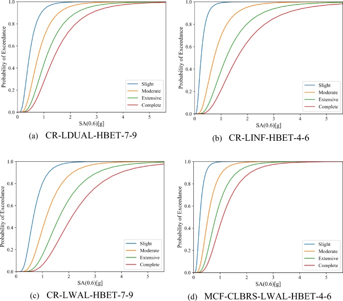
Fragility curve of typical building classes. a Reinforced concrete moment resisting frame with concrete shear walls structure 7 and 9 stories; b reinforced concrete moment resisting frame with infill walls structure 4 and 6 stories; c reinforced concrete shear wall structure 4 and 6 stories; d confined masonry structure 4 and 6 stories
-
(5)
The vulnerability models (probability of loss ratio conditional on ground shaking) are built based on the damage-to-loss model and proposed fragility models (Martins and Silva 2021), according to Eq. 6. The vulnerability models of typical buildings are illustrated in Fig. 15.
Fig. 15 
Vulnerability model of typical building classes. a Reinforced concrete moment resisting frame with concrete shear walls structure 7 and 9 stories; b Reinforced concrete moment resisting frame with infill walls structure 4 and 6 stories; c Reinforced concrete shear wall structure 4 and 6 stories; d Confined masonry structure 4 and 6 stories
$$\begin{array}{c}E\left[\left.LR\right|IM\right]=\sum_{i=1}^{nDS}\sum_{j=1}^{m}\left(P\left[DS={ds}_{i}\left|IM\right.\right] \times {LR}_{i,j} \times P\left[{LR}_{i,j}\right]\right)\end{array}$$(6)


\(P\left[DS={ds}_{i}\left|IM\right.\right]\) is the probability of occurrence of damage state \({ds}_{i}\) under IM conditions (calculated from the fragility function), and \({LR}_{i,j}\) and \(P\left[{LR}_{i,j}\right]\) represent the possible loss ratio for damage state \({ds}_{i}\) and its occurrence probability, which can be obtained from the damage-loss model.
5 Probabilistic Seismic Risk Results
The probabilistic seismic risk analysis was conducted for the Beijing–Tianjin–Hebei region using a stochastic event-based method. We combined the seismic hazard model, exposure model, and vulnerability model, and simulated a 100,000-year set of stochastic event based on the OpenQuake engine (Silva et al. 2014).
We combined the information from each stochastic rupture scenario with the GMPE of the corresponding seismotectonic zone. This approach allowed us to calculate the spatial distribution of the seismic hazard, thereby forming the corresponding ground motion field. Furthermore, in this study, we used Vs30 to account for the influence of site conditions on the ground motions. Finally, we calculated the corresponding losses by evaluating the vulnerability model curves of the exposed asserts in the affected area, which helped us form the spatial loss distribution.
The spatial loss distribution was used to calculate the risk metrics, for example, average annual loss (AAL) and exceedance probability curve (EP). The AAL was calculated by total losses in each subdistrict and dividing by the specific time period:
where \(T\) is the simulation time period, \(k\) is the number of events, and \({L}_{i}\) is the portfolio loss of each event \(i\).
The EP curve was used to illustrate the probability of exceeding a certain loss level in a given period:
where \(\uplambda \left(L>l\right)\) stands for the rate of exceedance of the respective loss \(l\), \(n(L>l)\) stands for the number of exceedances of the given loss \(l\), \(N\) is the number of events in time span. By assuming that the model conforms to the Poisson distribution, the exceedance probability that the loss exceeds \(l\) in period T can be calculated by Eq. 9.
Table 4 presents the residential replacement cost (construction cost), GDP, AAL, and average annual loss ratio (AALR, defined as average annual loss/replacement cost) for major cities in the Beijing–Tianjin–Hebei region.
In terms of AAL, the highest losses are in Beijing, Tianjin, and Tangshan, respectively. These cities are also the most developed in the region, as measured by their GDP. However, when we used AALR for ranking, the cities with the highest AALR are Tangshan (1.2‰), Beijing (0.9‰), Tianjin (0.8‰), and Langfang (0.8‰), respectively. This demonstrates that these four cities are at the highest risk within the region in terms of residential exposure. From a regional perspective, the AAL for the Beijing–Tianjin–Hebei region is RMB 3.715 billion yuan, with an AALR up to 6.3‰. This indicates a high seismic risk in the region.
Figure 16 illustrates the spatial distribution of the AALR in the Beijing–Tianjin–Hebei region to indicate the relative seismic risk level of residential replacement costs in each subdistrict. The overall distribution pattern reveals a clear spatial trend associated with the region’s major active faults, including the Tangshan Fault, the Xiadian Fault, and the Xinhe Fault. This pattern suggests that Tangshan, Beijing, Tianjin, Langfang, and Xingtai are area of relatively high seismic risk.

Map of average annual loss ratio (AALR) for the Beijing–Tianjin–Hebei region
Figure 17 presents the loss exceedance probability curve for the Beijing–Tianjin–Hebei region. The expected loss for return periods of 50, 100, and 1,000 years is RMB 36.6 billion yuan (6.3% replacement cost), RMB 62.7 billion yuan (10.79% replacement cost), and RMB 204.8 billion yuan (35.25% replacement cost), respectively. This is only the reconstruction cost of residential buildings, excluding contents costs. This illustrates the potentially serious impact of a rare earthquake on the regional economic system. The figure also depicts the EP curves for 15% and 85% quantiles. A notable finding is the growing difference between these two curves with the increasing return period, with a maximum difference of RMB 130 billion yuan, accounting for 37.3% of the mean loss value. This finding suggests that relying solely on the mean value as a metric for risk decision making and insurance scheme design could lead to significant repercussions.

The loss exceedance probability curve of the Beijing–Tianjin–Hebei region with mean and 15% and 85% quantiles
6 Discussion
It is crucial to acknowledge the limitations of our model. While our study accounted for the diversity of building structure characteristics and construction practices, certain assumptions were inevitably made due to data scarcity at a regional level. Although Vs30 serves as a primary proxy for site response in seismic design code and GMPEs, it offers a simplified representation of the site condition. Because the site condition can be much more complex, this simplification may lead to inaccuracies. In situations where the subsurface conditions contain layers of markedly different stiffness, or where the soil structure demonstrates a complex stratigraphy, there can be substantial variability in predicted values by GMPEs.
To capture and handle epistemic uncertainty, we applied the logic tree method in this study, incorporating HF19 and four models—ASK14, BSSA14, CB14, and CY14—from the NGA-West2 project. While these models were developed independently by different teams and utilized distinct modeling techniques, they exhibit variability in their functional form, parameterization, and assumptions. However, these GMPEs, which were developed based on the same datasets, can exhibit shared biases and limitations. These shared factors can potentially lead to correlated uncertainties among the GMPEs, which may, in turn, reduce the overall diversity and robustness of the logic tree approach. We acknowledge this limitation and our hazard estimates will not capture the whole uncertainty.
Seismic risk assessments are the results of a complex system with input from various sources. Inevitably, they involve certain assumptions, particularly in areas where data are limited. The accuracy of such models can be greatly improved with the availability of field surveys, empirical damage data, and experimental data. Therefore, the assessment results of our study should be regarded as rough indications and used with caution until more comprehensive data can be incorporated.
7 Conclusion
This study aimed to develop a probabilistic seismic risk model for the Beijing–Tianjin–Hebei region of China, which includes the exposure model, the vulnerability model, and the hazard model. The impact of site conditions and epistemic uncertainty from the seismic hazard model are taken into account. We used the stochastic event set method to assess this region’s seismic risk, deriving the AAL, AALR, loss exceedance probability curve, and seismic risk map. These can inform improvements to the national seismic design map, the formulation of seismic risk reduction objectives, evaluations of mitigation measures’ effectiveness, and the creation of public-private financial mechanisms for risk sharing and risk transfer.
Our analysis suggests that the replacement cost in the Beijing–Tianjin–Hebei region is RMB 5.81 trillion yuan (residential buildings). Of the values, 59% are located in the high intensity zone and 3% located in the zone with PGA greater than or equal to 0.3 g. The calculated average annual loss (AAL) in the region is RMB 3.715 billion yuan, representing 0.63% of the total replacement cost. Furthermore, the estimated probable maximum losses for return periods of 50, 100, and 1,000 years are RMB 36.6 billion yuan (6.3% replacement cost), RMB 62.7 billion yuan (10.79% replacement cost), and RMB 204.8 billion yuan (35.25% replacement cost), respectively. These figures suggest that the seismic risk in the Beijing–Tianjin–Hebei region should be given high importance. Importantly, a seismic hazard analysis alone cannot fully capture the seismic risk distribution in the region and is not sufficient as a basis for earthquake risk management and planning. The rare seismic events could significantly impact the regional economy, underscoring the importance of robust disaster preparedness and response mechanisms. Intriguingly, the loss ratio distribution in the region mirrors the geometry of major active seismic ruptures.
From a city-specific perspective, Tangshan, Beijing, Tianjin, and Langfang emerged as the highest-risk areas in the Beijing–Tianjin–Hebei region. The AALR for these cities are 1.2‰, 0.9‰, 0.8‰, and 0.8‰, respectively. Among these cities, Langfang exhibits the lowest level of economic development, as measured by GDP, and its AALP exceeds 1.5‰. This indicates that Langfang could face significant challenges in mobilizing adequate resources to respond to and recover from seismic events. To address such disparities, we recommend the establishment of an inter-regional disaster coordination mechanism. This would facilitate resource sharing, joint planning, and coordinated response efforts, thereby enhancing the region’s resilience to disasters.
Our findings indicate that the uncertainty of the loss exceedance probability curve increases with the return period. This is evidenced by a maximum difference of up to RMB 130 billion yuan (at the return period of 10,000 years) between the 15% and 85% quantiles, amounting to 37.3% of the mean loss. Seismic events are typically dominated by major earthquakes at high return periods. However, it often lacks sufficient data within this period range to constrain the model accurately. This deficiency contributes to escalating uncertainty within the models. This suggests that relying solely on the mean value for risk decision making and catastrophe insurance scheme designs could result in substantial biases. Thus, it is critical to account for the effects of uncertainty in seismic risk analysis. There is a profound need for future, in-depth research aimed at devising methodologies to quantify and limit the inherent uncertainty associated with tail risk.
Notes
https://db.world-housing.net, accessed in November 2022.
References
Abrahamson, N.A., W.J. Silva, and R. Kamai. 2014. Summary of the ASK14 ground motion relation for active crustal regions. Earthquake Spectra 30: 1025–1055.
Allen, T.I., and D.J. Wald. 2009. On the use of high-resolution topographic data as a proxy for seismic site conditions (VS 30). Bulletin of the Seismological Society of America 99: 935–943.
Amendola, C., and D. Pitilakis. 2023. Urban scale risk assessment including SSI and site amplification. Bulletin of Earthquake Engineering 21: 1821–1846.
Atkinson, G.M., and J. Adams. 2013. Ground motion prediction equations for application to the 2015 Canadian national seismic hazard maps. Canadian Journal of Civil Engineering 40: 988–998.
Avital, M., R. Kamai, M. Davis, and O. Dor. 2018. The effect of alternative seismotectonic models on PSHA results – A sensitivity study for two sites in Israel. Natural Hazards and Earth System Sciences 18: 499–514.
Baker, J., B. Bradley, and P. Stafford. 2021. Seismic hazard and risk analysis. Cambridge, UK: Cambridge University Press.
Bommer, J.J., J. Douglas, F. Scherbaum, F. Cotton, H. Bungum, and D. Fah. 2010. On the selection of ground-motion prediction equations for seismic hazard analysis. Seismological Research Letters 81(5): 783–793.
Bommer, J., R. Spence, M. Erdik, S. Tabuchi, N. Aydinoglu, E. Booth, D. del Re, and O. Peterken. 2002. Development of an earthquake loss model for Turkish catastrophe insurance. Journal of Seismology 6: 431–446.
Boore, D. 2004. Estimating Vs(30) (or NEHRP site classes) from shallow velocity models (depths < 30 m). Bulletin of the Seismological Society of America 94(2): 591–597.
Boore, D.M., J.P. Stewart, E. Seyhan, and G.M. Atkinson. 2014. NGA-West2 equations for predicting PGA, PGV, and 5% damped PSA for shallow crustal earthquakes. Earthquake Spectra 30: 1057–1085.
Borcherdt, R.D. 1994. Estimates of site-dependent response spectra for design (methodology and justification). Earthquake Spectra 10(4): 617–653.
Bradley, B.A. 2012. A ground motion selection algorithm based on the generalized conditional intensity measure approach. Soil Dynamics and Earthquake Engineering 40: 48–61.
BSSC (Building Seismic Safety Council). 2004. NEHRP recommended provisions for seismic regulations for new buildings and other structures, Part 1: Provisions (FEMA 450–1/2003 edition). Washington, DC: Building Seismic Safety Council.
Calvi, G.M., R. Pinho, G. Magenes, J.J. Bommer, L.F. Restrepo-Vélez, and H. Crowley. 2006. Development of seismic vulnerability assessment methodologies over the past 30 years. ISET Journal of Earthquake Technology 43(3): 75–104.
Campbell, K.W., and Y. Bozorgnia. 2014. NGA-West2 ground motion model for the average horizontal components of PGA, PGV, and 5% damped linear acceleration response spectra. Earthquake Spectra 30: 1087–1114.
Chen, H. 2013. General development and design of HAZ – China Earthquake Disaster Loss Estimation System. Recent Developments in World Seismology 2013(3): 45–47 (in Chinese).
Chen, X., X. Lin, L. Zhang, and K.A. Skalomenos. 2022. Method for rapidly generating urban damage scenarios under non-uniform ground motion input based on matching algorithms and time history analyses. Soil Dynamics and Earthquake Engineering 152: Article 107055.
Cheng, J., Y. Rong, H. Magistrale, G. Chen, and X. Xu. 2017. An Mw-based historical earthquake catalog for mainland China. Bulletin of the Seismological Society of America 107: 2490–2500.
Chiou, B.S.J., and R.R. Youngs. 2014. Update of the Chiou and Youngs NGA model for the average horizontal component of peak ground motion and response spectra. Earthquake Spectra 30: 1117–1153.
Cornell, C.A. 1968. Engineering seismic risk analysis. Bulletin of the Seismological Society of America 58(5): 1583–1606.
Crowley, H., J.J. Bommer, R. Pinho, and J. Bird. 2005. The impact of epistemic uncertainty on an earthquake loss model. Earthquake Engineering Structural Dynamics 34(14): 1653–1685.
Crowley, H., V. Despotaki, D. Rodrigues, V. Silva, D. Toma-Danila, E. Riga, A. Karatzetzou, and S. Fotopoulou. 2020. Exposure model for European seismic risk assessment. Earthquake Spectra 36: 252–273.
D’Ayala, D., and E. Speranza. 2003. Definition of collapse mechanisms and seismic vulnerability of historic masonry buildings. Earthquake Spectra 19: 479–509.
Danciu, L., Ö. Kale, and S. Akkar. 2018. The 2014 earthquake model of the Middle East: Ground motion model and uncertainties. Bulletin of Earthquake Engineering 16: 3497–3533.
Dangkua, D.T., Y. Rong, and H. Magistrale. 2018. Evaluation of NGA-West2 and Chinese ground-motion prediction equations for developing seismic hazard maps of mainland China. Bulletin of the Seismological Society of America 108: 2422–2443.
Dong, W. 2002. Engineering models for catastrophe risk and their application to insurance. Earthquake Engineering and Engineering Vibration 1(1): 145–151.
Friedman, D.G. 1972. Insurance and the natural hazards. ASTIN Bulletin: The Journal of the IAA 7(1): 4–58.
Friedman, D.G. 1984. Natural hazard risk assessment for an insurance program. Geneva Papers on Risk and Insurance 9(30): 57–128.
Gao, M., X. Li, and X. Xu. 2015. GB18306-2015: Introduction to the seismic hazard map of China. Beijing, China: Standards Press of China (in Chinese).
Grossi, P., H. Kunreuther, and D. Windeler. 2005. An introduction to catastrophe models and insurance. In Catastrophe modeling: A new approach to managing risk, ed. P. Grossi, and H. Kunreuther, 23–42. New York: Springer.
Grossi, P., D.D. Re, Z. Wang, and K. Lao. 2006. The 1976 Great Tangshan Earthquake: 30-year retrospective. Plymouth, MN: RMS Inc.
He, C., Q. Huang, Y. Dou, W. Tu, and J. Liu. 2017. The population in China’s earthquake-prone areas has increased by over 32 million along with rapid urbanization. Environmental Research Letters 12: Article 039501.
Hong, H.P., and C. Feng. 2019. On the ground-motion models for Chinese seismic hazard mapping. Bulletin of the Seismological Society of America 109: 2106–2124.
Iwahashi, J., and R.J. Pike. 2007. Automated classifications of topography from DEMs by an unsupervised nested-means algorithm and a three-part geometric signature. Geomorphology 86: 409–440.
Jalayer, F., R. De Risi, and G. Manfredi. 2015. Bayesian cloud analysis: Efficient structural fragility assessment using linear regression. Bulletin of Earthquake Engineering 13: 1183–1203.
Jiang, J., and F. Hong. 1985. Seismic reliability analysis of multi-story brick building. Earthquake Engineering and Engineering Vibration No. 4: 13–28 (in Chinese).
Joyner, W.B., and D.M. Boore. 1988. Measurement, characterization, and prediction of strong ground motion. In Earthquake engineering and soil dynamics II: Recent advances in ground-motion evaluation. Proceedings of the American Society of Civil Engineers Geotechnical Engineering Division Specialty Conference, 27–30 June 1988, Park City, UT, USA, 27–30.
Lemoine, A., J. Douglas, and F. Cotton. 2012. Testing the applicability of correlation between topographic slope and VS30 for Europe. Bulletin of Seismological Society of America 102: 2585–2599.
Ma, J. 2022. Research on the regional probabilistic seismic risk model development and sensitivity analysis. Ph.D. dissertation. Beijing: Beijing Normal University (in Chinese).
Ma, J., A. Rao, V. Silva, K. Liu, and M. Wang. 2021. A township-level exposure model of residential buildings for mainland China. Natural Hazards 108: 389–423.
Martins, L., and V. Silva. 2021. Development of a fragility and vulnerability model for global seismic risk analyses. Bulletin of Earthquake Engineering 19: 6719–6745.
Massa, M., S. Barani, and S. Lovati. 2014. Overview of topographic effects based on experimental observations: Meaning, causes and possible interpretations. Geophysical Journal International 197(3): 1537–1550.
McGuire, R.K. 1995. Probabilistic seismic hazard analysis and design earthquakes: Closing the loop. Bulletin of the Seismological Society of America 85(5): 1275–1284.
McKenna, F. 2011. OpenSees: A framework for earthquake engineering simulation. Computing in Science and Engineering 13: 58–66.
Mitchell-Wallace, K., M. Jones, J. Hillier, and M. Foote. 2017. Natural catastrophe risk management and modelling: A practitioner’s guide. Hoboken, NJ: John Wiley & Sons.
Musson, R.M.W. 1999. Determination of design earthquakes in seismic hazard analysis through Monte Carlo simulation. Journal of Earthquake Engineering 3(4): 463–474.
Pagani, M., D. Monelli, G. Weatherill, L. Danciu, H. Crowley, V. Silva, P. Henshaw, and L. Butler et al. 2014. OpenQuake engine: An open hazard and risk software for the global earthquake model. Seismological Research Letters 85(3): 692–702.
Rossetto, T., I. Ioannou, and D.N. Grant. 2015. Existing empirical fragility and vulnerability functions: Compendium and guide for selection. GEM Technical Report 2015-1. Pavia, Italy: GEM Foundation.
Silva, V., D. Amo-Oduro, A. Calderon, C. Costa, J. Dabbeek, V. Despotaki, and M. Pittore. 2020. Development of a global seismic risk model. Earthquake Spectra 36(S1): 372–394.
Silva, V., H. Crowley, M. Pagani, D. Monelli, and R. Pinho. 2014. Development of the OpenQuake engine, the Global Earthquake Model’s open-source software for seismic risk assessment. Natural Hazards 72: 1409–1427.
Strasser, F.O., J.J. Bommer, K.A.R.İN. Şeşetyan, M. Erdik, Z. Çağnan, J. Irizarry, X. Goula, and A. Lucantoni et al. 2008. A comparative study of European earthquake loss estimation tools for a scenario in Istanbul. Journal of Earthquake Engineering 12(S2): 246–256.
Villar-Vega, M., V. Silva, H. Crowley, C. Yepes, N. Tarque, A.B. Acevedo, M.A. Hub, and C.D. Gustavo et al. 2017. Development of a fragility model for the residential building stock in South America. Earthquake Spectra 33: 581–604.
Wald, D.J., and T.I. Allen. 2007. Topographic slope as a proxy for seismic site conditions and amplification. Bulletin of the Seismological Society of America 97: 1379–1395.
Wieland, M., M. Pittore, S. Parolai, J. Zschau, B. Moldobekov, and U. Begaliev. 2012. Estimating building inventory for rapid seismic vulnerability assessment: Towards an integrated approach based on multi-source imaging. Soil Dynamics and Earthquake Engineering 36: 70–83.
Woessner, J., D. Laurentiu, D. Giardini, H. Crowley, F. Cotton, G. Grünthal, G. Valensise, and R. Arvidsson et al. 2015. The 2013 European Seismic Hazard Model: Key components and results. Bulletin of Earthquake Engineering 13: 3553–3596.
Wu, J., C. Wang, X. He, X. Wang, and N. Li. 2017. Spatiotemporal changes in both asset value and GDP associated with seismic exposure in China in the context of rapid economic growth from 1990 to 2010. Environmental Research Letters 12(3): Article 034002.
Xie, Z., Y. Lv, Y. Fang, and B. Shi. 2017. Relocated seismicity and its relation with active faults in Beijing-Tianjin-Hebei area. Earthquake 37(3): 72–83 (in Chinese).
Xiong, C., X. Lu, J. Huang, and H. Guan. 2019. Multi-LOD seismic-damage simulation of urban buildings and case study in Beijing CBD. Bulletin of Earthquake Engineering 17: 2037–2057.
Yepes-Estrada, C., V. Silva, J. Valcárcel, A.B. Acevedo, N. Tarque, M.A. Hube, G. Coronel, and H.S. María. 2017. Modeling the residential building inventory in South America for seismic risk assessment. Earthquake Spectra 33: 299–322.
Yin, Z. 1994. A dynamic model for predicting earthquake disaster losses. Journal of Natural Disasters 3(2): 72–80 (in Chinese).
Yu, X., and D. Lu. 2016. Probabilistic seismic demand analysis and seismic fragility analysis based on a cloud-stripe method. Engineering Mechanics 33: 68–76 (in Chinese).
Yu, Y.X., S.Y. Li, and L. Xiao. 2013. Development of ground motion attenuation relations for the new seismic hazard map of China. Technology for Earthquake Disaster Prevention 8(1): 24–33 (in Chinese).
Zhang, L., J. Jiang, and J. Liu. 2002. Seismic vulnerability analysis of multistory dwelling brick buildings. Earthquake Engineering and Engineering Vibration 22: 49–55 (in Chinese).
Zhang, Y., Y. Ren, R. Wen, H. Wang, and K. Ji. 2023. Regional terrain-based VS 30 prediction models for China. Earth, Planets and Space 75(1): Article 72.
Zhang, Y., S. Zheng, L. Sun, L. Long, and L. Li. 2021. Developing GIS-based earthquake loss model: A case study of Baqiao District, China. Bulletin of Earthquake Engineering 19: 2045–2079.
Acknowledgments
The financial support received from the Scientific Research Fund of Institute of Engineering Mechanics, China Earthquake Administration (Grant No. 2023B09); National Key R&D Program of China (2022YFC3004404); and Shenzhen Science and Technology Program (ZDSYS20210929115800001) are gratefully acknowledged. We would like to thank Dr. Yefei Ren and Yuting Zhang from the Institute of Engineering Mechanics, China Earthquake Administration for sharing the Vs30 data of the study region. The authors thank three anonymous reviewers and journal editor.
Author information
Authors and Affiliations
Corresponding author
Rights and permissions
Open Access This article is licensed under a Creative Commons Attribution 4.0 International License, which permits use, sharing, adaptation, distribution and reproduction in any medium or format, as long as you give appropriate credit to the original author(s) and the source, provide a link to the Creative Commons licence, and indicate if changes were made. The images or other third party material in this article are included in the article's Creative Commons licence, unless indicated otherwise in a credit line to the material. If material is not included in the article's Creative Commons licence and your intended use is not permitted by statutory regulation or exceeds the permitted use, you will need to obtain permission directly from the copyright holder. To view a copy of this licence, visit http://creativecommons.org/licenses/by/4.0/.
About this article

Cite this article
Ma, J., Goda, K., Liu, K. et al. Seismic Risk Model for the Beijing–Tianjin–Hebei Region, China: Considering Epistemic Uncertainty from the Seismic Hazard Models. Int J Disaster Risk Sci (2024). https://doi.org/10.1007/s13753-024-00568-4
Accepted:
Published:
DOI: https://doi.org/10.1007/s13753-024-00568-4