
Abstract
Climate change has led to increasing frequency of sudden extreme heavy rainfall events in cities, resulting in great disaster losses. Therefore, in emergency management, we need to be timely in predicting urban floods. Although the existing machine learning models can quickly predict the depth of stagnant water, these models only target single points and require large amounts of measured data, which are currently lacking. Although numerical models can accurately simulate and predict such events, it takes a long time to perform the associated calculations, especially two-dimensional large-scale calculations, which cannot meet the needs of emergency management. Therefore, this article proposes a method of coupling neural networks and numerical models that can simulate and identify areas at high risk from urban floods and quickly predict the depth of water accumulation in these areas. Taking a drainage area in Tianjin Municipality, China, as an example, the results show that the simulation accuracy of this method is high, the Nash coefficient is 0.876, and the calculation time is 20 seconds. This method can quickly and accurately simulate the depth of water accumulation in high-risk areas in cities and provide technical support for urban flood emergency management.
1 Introduction
Global climate change has affected the intensity and patterns of rainfall, which in turn has affected runoff (May 2008; Hammond et al. 2015). This has led to frequent flooding, causing heavy economic losses and casualties (Banik et al. 2015). In July 2012, Beijing registered a flood emergency caused by road inundation. There was no immediate prediction of flooding, which would have enabled the implementation of appropriate actions and preventive measures, thereby resulting in 79 deaths (Yin et al. 2015). Failure to respond quickly to floods causes great losses, and rapid response is based on rapid and accurate forecasting. Quickly predicting flood disasters is a key component to providing decision makers with sufficient time to act and minimize disaster losses (María et al. 2020).
Urban flood forecasting research mainly focuses on two types of forecasting based on urban flood simulation models and time series analyses. Since the 1970s, urban flood models have been produced and developed rapidly and research on flood warning and prediction based on urban flood simulation models also began, and the technology is relatively mature. But a series of problems, such as limited understanding of hydrological and hydrodynamic processes, complex data requirements, and modeling difficulties, have restricted the application of the models (Zheng et al. 2014; Liu et al. 2015; Zanchetta and Coulibaly 2020). Huang et al. (2017) constructed a comprehensive urban drainage model based on InfoWorks ICM (Integrated Catchment Management) to simulate the drainage capacity and depth of the drainage network system in the main urban area of Haikou City under different rainstorm scenarios, providing a scientific basis for the optimization and transformation of the drainage network and supporting urban flood control and mitigation efforts. Zeng et al. (2017) coupled the storm water management model (SWMM), the one-dimensional pipe network model, and the LISFLOOD-FP two-dimensional hydrodynamic model to simulate the flooding range and depth of rainstorms, providing a reference for the study of flood early warnings. In recent years, many rapid flood inundation models have been put to use. Krupka (2009) constructed a rapid flood inundation model that can be used for flood prediction and flood risk management in urban areas based on a digital elevation model (DEM). Zhang and Pan (2014) proposed a GIS-based urban storm-inundation simulation method based on the simplification of the distributed hydrological model, which can quickly calculate the submerged depth and area. At present, physics-based simulation models require a long calculation time, which is the bottleneck of rapid flood analysis (Leitao et al. 2010). This problem becomes more prominent when running simulations over large areas or at high spatial resolutions. Because of the higher resolution required in urban areas, the feasible simulation scale for numerical models is much smaller. Although the physical model has been greatly improved in the application of large-scale urban models, the current state-of-the-art simulation methods are still not fast enough, especially for applications that require iterative analysis (Guo et al. 2015). This emphasizes the need to develop rapid flood forecasting tools that can be used for urban flood risk management and urban planning.
Compared with physical models, the flood warning and forecasting method based on time series analysis is simple to model and has lower requirements for understanding hydrological and hydraulic laws. It has great potential in research on urban flood warning and forecasting (Mounce et al. 2014; Zhang et al. 2019; Wei et al. 2020). Zheng et al. (2014) improved the spatial and temporal autoregressive and moving average model (STARMA) of rainfall and stagnant water and made short-term predictions of the stagnant water process in urban rainstorms. Rjeily et al. (2017) developed a flooding forecast system (FFS) based on a nonlinear automatic regression with external inputs (NARX) neural network to alert urban drainage system managers to possible flooding in advance. Yan et al. (2018) used a numerical model as a data generator and developed two support vector machine (SVM) models, which were used to predict flooding and the maximum flooding depth, and effectively provided urban flood warning. She and You (2019) coupled the radial basis function (RBF) and NARX to build a model for predicting urban drainage curves, which has great potential in urban runoff prediction and management. Wu et al. (2020) used 16 combinations of rainfall sensitivity indicators to determine the optimal plan for predicting the depth of stagnant water and used the gradient boosting decision tree (GBDT) algorithm in deep learning to construct the urban storm gathering point of the stagnant process prediction model, generating refined forecasts of urban floods. Lee et al. (2020) used machine learning methods combined with design rainfall-runoff analysis (DRRA) and watershed characteristics to estimate appropriate design floods for unmeasured watersheds. The data-driven model proposed by them can help improve flood response capabilities. Although machine learning methods are widely used in flood forecasting, most of these studies focus on single-point flood level prediction. In addition, most of the research on spatial flood forecasting is based on numerical models. Based on a single point forecast, the distribution of floods cannot be shown, and based on the prediction of digital simulation the time required for refined simulation is longer.
Due to the general lack of measured inundation data in China, it is difficult to conduct a preliminary analysis of floods in urban areas. In recent years, some researchers have begun to try to use a combination of numerical simulation models and machine learning methods. In response to the demand for rapid and probabilistic flood modeling, Li and Willems (2020) proposed a hybrid modeling method that combines a lumped hydrological model with logistic regression. Hou et al. (2021) used a hydrodynamic model with a 2D shallow water equation as the governing equation, and proposed a rapid prediction model combining a hydrodynamic model and machine learning algorithm. Kabir et al. (2020), using the two-dimensional hydraulic model LISFLOOD-FP, proposed a rapid flood prediction method based on deep convolutional neural networks. Kim and Han (2020) established a flood scenario database using a SWMM and a two-dimensional hydraulic analysis program FLO-2D based on the finite difference method, and proposed a real-time urban flood prediction method based on the drainage district of a large city. Lee and Kim (2021) used a FLO-2D model and logistic regression to predict the flood range. The numerical models used in these studies mostly import the calculation results of the one-dimensional model into a two-dimensional hydraulic analysis program based on the finite difference method for simulation or directly use a two-dimensional hydrodynamic model that can only simulate surface flooding. However, this study only uses a single numerical simulation model to achieve one- and two-dimensional coupling, which has a higher degree of coupling. At present, there is no research on the use of the personal computer storm water management model (PCSWMM) for rapid urban flood prediction. The PCSWMM of the Canadian Hydraulic Computational Research Institute has a powerful hydrology and hydraulics module that can calculate rainfall and surface runoff and hydrodynamic transportation in pipeline networks, support low-impact development modeling and 1D-2D coupling modeling, and simulate the complete rainfall-runoff process, and the simulation results have high accuracy.
Therefore, this study coupled a two-dimensional hydrological and hydrodynamic model with a statistical analysis model and proposed a spatiotemporal maximum water depth prediction method based on neural network-numerical simulation. The Elman neural network was used to learn and memorize the mapping relationship from the input rainfall scenario to the output maximum water depth, and the single point water depth to the output water depth of each point in the rest of the space. The Elman neural network was trained using the simulation result dataset of 35 design rainfall scenarios with 5 design rain patterns and 7 return periods in the downtown area of Tianjin Municipality, China. This study combined traditional neural network prediction methods with urban flood simulation models to predict the time and space of urban water accumulation and verify the designed and actual rainfall events.
Section 2 outlines the method employed in this study; Sect. 3 describes the study area, the data used, and the case study results; and a brief discussion and conclusion are provided in Sects. 4 and 5.
2 Methods
This section introduces the relevant principles of the PCSWMM and Elman neural network models, explains the selection of multiscenario design rain patterns in this study, and summarizes the framework for rapid flood forecasting in high-risk areas.
2.1 Urban Flood Simulation Model Based on the Personal Computer Storm Water Management Model (PCSWMM)
The PCSWMM is a hydrological and hydraulic model developed by the Canadian Hydraulic Computational Research Institute with a SWMM as the core. It has been widely used in one-dimensional pipeline and two-dimensional floodplain coupling simulation, drainage network design and evaluation, flood storage design and evaluation, flood risk analysis, and other fields. The PCSWMM software has advanced simulation calculation methods and convenient operation, which is more suitable for urban drainage modeling (Ahiablame and Shakya 2016; Beck 2016; Wu and Huang 2016). Therefore, this study was based on the PCSWMM to establish urban one-dimensional and two-dimensional coupled flood simulation models that make it easier to extract inundation information.
The free flow of water along the two-dimensional surface adopts the complete dynamic wave method, and the governing equations of the pipeline and channel include the continuity equation and momentum equation.
where x is the length, m; A is the flow area, m2; Q is the flow, m3/s; H is the head, m; Sf is the friction slope, m/m; hL is the local head loss per unit length, m/m; and g is the acceleration due to gravity, m/s2.
In this study, the infiltration model selected was the Horton model, and the infiltration formula is:
where ft is the infiltration rate at time t, mm/h; f0 is the maximum infiltration rate, mm/h; fc is the stable infiltration rate, mm/h; β is the infiltration attenuation coefficient, mm/h; and t is the infiltration time, h.
In the PCSWMM neutron catchment area, the one-dimensional dynamic wave model was used to calculate the flow of runoff reaching the gully and the water flow in the pipeline network. The two-dimensional model was used to travel along the surface after the water overflows from the manhole and the river.
2.2 Multiscenario Design Rain Type Selection
At present, the integrated management of hydrology, coupled with water resources, rainstorms, and floods, requires true and complete meteorological and hydrological data. The characteristics of rainfall, especially its temporal distribution and intensity, have a great influence on the simulation of rainfall, runoff, and flood events. A large part of the errors in the rainfall-runoff-flood model simulation is due to the uncertainty of the regional rainfall pattern (Moulin et al. 2009). Therefore, it is very important to use the rainfall data of each region to provide the rainfall distribution pattern in that region because this pattern is different in regions with different climates. When Huff (1967) studied the torrential rainfall patterns in Illinois, United States, he proposed dividing rainstorms into four categories according to the location of the rainfall peak, and obtaining the average dimensionless accumulation process of the various rainfall patterns. Keifer and Chu (1957) proposed the Chicago rain pattern based on the relationship between rainfall intensity and duration, which is applicable to various torrential rain processes. Taking into account the impact of the location of the rainfall peak on rainfall accumulation, and following the principle that the rainfall-accumulation database should be as universal and representative as possible, this study used the Huff rain pattern and the commonly used Chicago rain pattern as the basic rain pattern. By combining the rainfall of different return periods in this area, the obtained multiple rainfall scenarios were used as the boundary input conditions of the flood simulation model.
2.3 Elman Neural Network Algorithm
According to the flow of information during the operation of the neural network, the neural network can be divided into two basic types: feedforward and feedback. Compared with the feedforward neural network, the feedback neural network is a potential choice that can directly reflect the dynamic characteristics of the system (Meng et al. 2009).
The Elman neural network is a dynamic recursive neural network. It adds a connecting layer to the hidden layer based on the back propagation (BP) neural network to achieve the purpose of memory so that the network has the ability to adapt to the characteristics of events and increase the global stability of the network. The Elman network structure is divided into four layers: input layer, connected layer, hidden layer, and output layer. The structure of the input, hidden, and output layers is similar to a feedforward network. The input layer is used for signal transmission. The connected layer is used to memorize the output value of the hidden layer at the previous moment. The output of the hidden layer is self-connected to the input of the hidden layer through the connected layer. This method makes it sensitive to historical data to achieve dynamic modeling. The network structure and calculation process are shown in Fig. 1.

The Elman neural network structure
The nonlinear state space expression of the Elman neural network is:
where y is the m-dimensional output node vector; x is the n-dimensional hidden layer node unit vector; u is the r-dimensional input vector; xc is the n-dimensional feedback state vector; ω3 is the connection weight from the hidden layer to the output layer; ω2 is the connection weight from the input layer to the hidden layer; ω1 is the connection weight from the context layer to the hidden layer; g(*) is the transfer function of the output neuron, which is the linear combination of the output of the hidden layer; f(*) is the transfer function of the hidden layer neuron, and the S function is used frequently in it. The Elman neural network also uses the BP algorithm for weight correction, and the learning index function uses the error square sum function.
where \({\tilde{\text{y}}}_{\text{k}}(\omega) \) is the target input vector.
2.4 Framework for the Rapid Prediction of Floods Combined with Neural Networks and Numerical Simulations
The rapid prediction method of floods combined with neural networks and numerical simulations mainly includes the establishment of urban flood simulation models, statistics of rainfall scenarios, selection of high-risk points, single-point water accumulation depth prediction, and other high-risk point water accumulation depth predictions. The framework of the method is shown in Fig. 2. In principle, the water depth of a single point is predicted from the rainfall scenario sequence, and then the water depth of the remaining spatial points is predicted from the water depth of one point. In application, it is only necessary to input the rainfall scenario sequence and extract the spatial coordinate value of each high-risk point; then, the maximum water depth of each high-risk point corresponding to the coordinate can be quickly output.

Framework of the predictive model of urban flood inundation based on neural network-numerical simulation. DEM = digital elevation model; PCSWMM = personal computer storm water management model.
2.4.1 Prediction of Single Point Maximum Water Depth Based on an Elman Neural Network
Urban stagnant water caused by heavy rain will be affected by many factors, including rainfall processes, underlying surfaces, drainage systems, and river distribution. Even the same spatial location in different rainfall events and the rainfall accumulation process of different spatial locations under the same rainfall event are very different. Therefore, in the absence of historical hydrological data and basic environmental data, it is very difficult to carry out urban stagnant water prediction research through methods based on hydrological and hydrodynamic principles, statistical principles, and urban rain and flood models. It is difficult to ensure accurate predictions due to the considerable simulation time required (Kim et al. 2019). However, the prediction of stagnant water characteristics based on neural networks is not limited by such problems. In this method, the input of different rainfall processes and the maximum water depth output of high-risk flood points are constructed as a training database. The neural network is used as the medium of the relationship between the two, and the mapping relationship between input and output functions is determined by training through the constructed database samples. Based on this, the corresponding rapid prediction model of stagnant water is established.
The rapid prediction method of urban stagnant water based on the Elman neural network mainly includes four processes: the construction of the prediction database, model training, model prediction, and model prediction result analysis. The framework for the rapid prediction of urban stagnant water based on the Elman neural network is shown in Fig. 3.

A framework for the rapid prediction of urban stagnant water based on the Elman neural network
The data required for the model established in this study include rainfall time series and maximum water depth at high-risk points. The rainfall time series should be the n-part rainfall process of a specific duration in the study area, and the rainfall process should refer to the historical rainfall events in the area as much as possible so that the established database is more representative. Using these rainfall time series as the input boundary conditions of the urban flood simulation model, the maximum submerged depth at the same high-risk point under different working conditions was obtained. Corresponding to the input rainfall and output water depth, a database matrix that can provide training samples for the fast water accumulation prediction model is formed.
Before the model training starts, the established database must be preprocessed. The preprocessing method used in this model is normalization. The purpose of normalization is to process data from different sources and dimensions to be unified under the same reference frame and transform the data of each indicator into the (0, 1) interval. After the data are normalized and preprocessed, the dataset needs to be divided into a training dataset and a test dataset. Based on previous experience, it is generally divided by a ratio of close to 7:3. After sample selection and processing, a neural network prediction model was built. This process mainly includes the process of determining the number of neural network layers, selecting the number of neuron nodes, model training, and prediction.
2.4.2 Prediction of Spatial Multipoint Water Accumulation Based on a Neural Network
Machine learning is gaining increasing attention in flood forecasting. However, most of these studies focus on time series predictions based on specific sensors, such as river water level and flow measured by hydrological stations and fixed-point water depth predictions at urban water monitoring stations (Zheng et al. 2014; Bowes et al. 2019; Wan et al. 2019). There are very few temporal and spatial predictions of floods available. In this study, based on the flood simulation model, a model framework integrating the Elman neural network and spatial point water depth was developed.
The spatiotemporal prediction model of urban floods combines the Elman neural network with fixed spatial points. First, a spatial coordinate system was built for the study area on Jiefang South Road, Tianjin, and a number of high-risk points was selected based on the flood inundation results simulated by the PCSWMM model, including the high-risk points for which the depth of stagnant water was predicted in Sect. 2.4.1. We built a prediction model with the known point depth as an input element. The depth element was used as the input of the water accumulation spatiotemporal prediction model, and the water depth of the remaining unknown points was used as the output for training. After the database was established, the data were normalized to transform the sample dataset into the (0, 1) interval. After processing, the dataset was divided between the training set and the test set by a ratio close to 7:3, and the training verification and prediction of the neural network model were then performed.
3 The Tianjin Case Study
This study took a drainage area in Tianjin as an example, coupled a two-dimensional hydrological and hydrodynamic model and a neural network model, and constructed a rapid prediction model for stagnant water in high-risk areas.
3.1 Study Area
The study area is a drainage area in Tianjin, south of the central city, in the area of Jiefang South Road, with an area of approximately 16.7 km2 (Fig. 4). The study area belongs to the alluvial plain in the lower reaches of the Haihe River Basin. The terrain is relatively flat, and the elevation does not exceed 3.5 m. The surface rainwater confluence process is relatively gentle. The urban built-up area is mainly drained by pipe network pumping stations. In addition, the groundwater level is high, the impervious area ratio is high, and the soil permeability coefficient is low. Many road sections are low-lying and flat and prone to flood disasters when affected by rainfall. The placement of stagnant water monitoring equipment is currently being planned for this area.

Schematic diagram of the location of the drainage area on Jiefang South Road in Tianjin Municipality, China
3.2 Establishment of the Rainfall Database and Water Depth Database of Spatial Points
To carry out research on the rapid forecast of accumulated water in the drainage area of Jiefang South Road in Tianjin based on the neural network algorithm, it is necessary to construct a rainfall-accumulated water database for this area first. The rainfall type adopts the Huff rain type and Chicago rain type, and the design rainstorm value refers to the Tianjin Sponge City Construction Technical Guidelines. Huang et al. (2020) used minute-by-minute rainstorm data for 54 years from 1951 to 2004, selected the three largest rainstorms each year for a total of 162, and analyzed the evolution of the designed rainstorm patterns in Tianjin.
According to the design principle of the Huff rain pattern, in the design of the rainfall pattern in the study area, the rainfall time series was divided into four categories according to the location of the rain peak, and the various types of rainfall were classified. Then, the average dimensionless accumulation process of various rain patterns can be obtained. In the study, each rainfall process was divided into 10 equal parts, and the proportion of the precipitation in each interval to the total was calculated separately. Then, according to the position of the rain peak during the rainfall, it was divided into first quarter, second quarter, third quarter, and fourth quarter rain patterns, which are referred to as rain types 1, 2, 3, and 4, respectively. In addition, the Chicago rain pattern is a single peak rain pattern, which is derived from the rainstorm intensity formula and the rain peak coefficient, and is called the rain type 5.
Different rainfall durations were divided into different rainfall duration events. The rainfall duration selected in this study is 3 h, which represents the rain pattern obtained from the rainfall data of 1–3 h, as shown in Fig. 5. Therefore, in this study, the design storm value adopted the rainfall distribution under the corresponding rainfall duration event to obtain the complete rainfall process. According to the Tianjin Sponge City Construction Guidelines, the design rainstorm intensity lasting 3 hours under different return periods is shown in Table 1. Thirty-five rainfall events obtained by combining different situations were used as the boundary conditions of the PCSWMM urban flood simulation model.

Design rain patterns adopted for the study area on Jiefang South Road in Tianjin Municipality, China (% of rain in 3 hours, divided into 10 intervals)
The essence of the spatial database is to combine the location information of the high-risk points to be predicted with the maximum water depth information. First, a rectangular spatial coordinate system was established in the study area, and according to the flooding results of the urban flood simulation model in the study area, as shown in Fig. 6, several water-accumulating points were selected from points at which the maximum inundation depth was greater than 5 cm, and their location information was extracted. Then, the maximum water depth corresponding to each spatial point was calculated under different rainfall scenarios.

Results of flooding in the study area on Jiefang South Road in Tianjin Municipality, China (the maximum water depth > 0.05 m)
This study selected seven high-risk points in the study area, and their spatial locations are shown in Fig. 7. Among them, point 1 is the high-risk point that was tested in the single-point maximum water depth prediction, that is, the points of known depth in the prediction of the maximum water depth in the area, and the remaining six points are the points to be predicted in the prediction method based on neural network-spatial coordinate water accumulation. First, the study area was georegistered with the geographic coordinate system WGS 1984 and then processed in ArcGIS software to extract the coordinate information of the remaining six points. The results are shown in Table 2.

Spatial location of the water depth prediction points in the study area on Jiefang South Road in Tianjin Municipality, China. X refers to Xiufangli rainfall station in Tianjin Municipality, China.
The seven high-risk points were entered in the PCSWMM software. The water depth of each point in the 35 rainfall scenarios was extracted assuming that the rain intensity that occurs once in two years is allocated according to rain pattern 1. Then, the scenario is named 21, and the rest can be deduced by analogy. The corresponding maximum water depth of each spatial point forms a sample matrix of 35 spatial water accumulation predictions to construct a spatial point water depth prediction database.
3.3 Construction of an Urban Rainstorm and Flood Model
To construct a two-dimensional coupled flood simulation model for the drainage area in Tianjin, a one-dimensional drainage model needs to be constructed first. On the basis of the one-dimensional drainage model, the orifice layer was added to realize the interaction of the water volume of the aboveground and underground drainage systems to obtain one- and two-dimensional coupled flood simulation models.
To verify whether the simulation results of the model can accurately reflect the situation in the study area, the model needs to be calibrated and verified to achieve the best simulation effect. The model calibration process used the local rainfall data measured in 2019 and took the five flood monitoring stations in the area as the object for parameter calibration. The time interval is 1 hour. The process is shown in Fig. 8. The locations of the five stations (blue dots) for calibration are shown in Fig.7.

Rainfall process at Xiufangli rainfall station (from 21:00 on 1 August to 5:00 on 2 August 2019) in the study area on Jiefang South Road in Tianjin Municipality, China
Rainfall data were input into the constructed flood model for simulation, and the simulated flood situation after rainfall is shown in Fig. 6. The submerged area and submerged depth simulated by the model were extracted, the simulated data were compared with the measured data, and optimized debugging was performed to reduce the error of the model and obtain the optimal values of the relevant parameters. The calibrated parameters include the subcatchment area, characteristic width, average slope, proportion of impermeable area, Manning coefficient of impermeable area, Manning coefficient of permeable area, and depression storage in permeable and impermeable areas. The parameter values are shown in Table 3.
The comparison between the measured and simulated results is shown in Table 4. The measured depth of water accumulation at the five flood monitoring stations is 1.9–36.3 cm, and the simulated depth of the five stations is 1.6–37.1 cm.
To further judge the quality of the model simulation results, this study selected four quantitative indicators to evaluate the simulation results: the Nash-Sutcliffe efficiency coefficient (NSE) (Nash and Sutcliffe 1970), the root mean squared error (RMSE), the coefficient of determination (R2), and the peak relative error (PE). The calculation formulas are:
where \({\text{h}}_{\text{obs,i}}\) is the observed water depth at time i; \({\text{h}}_{\text{sim,i}}\) is the simulated water depth at time i; \({\text{h}}_{\text{obs,mean}}\) is the mean value of the observed water depth;\({\text{h}}_{\text{sim,mean}}\) is the mean value of the simulated water depth; \({\text{h}}_{\text{sim,peak}}\) is the peak value of the simulated water depth; and \({\text{h}}_{\text{obs,peak}}\) is the peak value of the observed water depth. The closer the NSE value is to 1, the higher the degree of agreement between the simulation result and the observed curve.
The NSE, RMSE, R2, and PE values of the model are 0.81, 5.24, 0.73, and 0.02, respectively. Based on Santhi et al. (2010), the error can be considered to be within the allowable range. Therefore, the flood model constructed in this study can reflect the flood process in the drainage area in the downtown area of Tianjin to a certain extent. Table 4 shows that the simulation results of stations B and D have large errors compared to the actual measurement. This may be caused by insufficient accuracy of the utilized DEM. The DEM of this model comes from the municipal department and has an accuracy of 19 m. For urban flood research, this resolution does not reach the high precision standard. At the campus (station B) and intersections in the study area, engineering renovation or construction may be carried out, resulting in changes in the surrounding ground conditions and elevation. However, the DEM data are not updated in real time, which causes errors in the model.
We also compared the simulation results at the maximum and minimum water accumulation points caused by the rainstorm process with the actual water accumulation occurring in the corresponding grid, as shown in Figs. 9 and 10. The NSE, RMSE, R2, and PE values for the water depths at station A are 0.89, 3.02, 0.98, and 0.02, respectively. The NSE, RMSE, R2, and PE values for the water depths at station E are 0.84, 0.21, 0.58, and 0.19, respectively. The analysis result shows that the model can simulate the water accumulation area in the urban area, but there is a certain deviation. The main reasons for the deviation are: (1) the generalization error of the drainage pipe network affects the accuracy of the calculation to a certain extent; (2) there are errors in the observation of actual water accumulation; and (3) the grid elevation is the average elevation of the terrain in the area, and it cannot reflect the water accumulation in locally low-lying areas.

Comparison between simulated and measured water processes (from 22:50 on 1 August to 4:30 on 2 August 2019) at station A in the study area on Jiefang South Road in Tianjin Municipality, China

Comparison between simulated and measured water processes (from 22:20 on 1 August to 1:00 on 2 August 2019) at station E in the study area on Jiefang South Road in Tianjin Municipality, China
3.4 Construction of the Elman Neural Network Model
First the number of neural network layers is determined and the number of neuron nodes is selected. Then the data pre-processed database is trained and verified to construct the Elman neural network stagnant water prediction model.
-
(1)
The number of neural network layers
In the Elman neural network structure, the optimization of the number of layers or the number of hidden layers can improve the prediction accuracy of the model, but when the complexity of the network structure is increased, the network training time needs to be extended accordingly. In this study, a network structure with a single hidden layer and a single successor layer was selected, and the prediction accuracy of the model was improved by appropriately changing the number of nodes of the hidden layer neurons.
-
(2)
Determination of the number of neurons
The appropriate selection of neuron nodes has a great impact on the network training results. Too few neuron nodes may result in a lower training result accuracy and larger errors. Too many neurons will increase the sample training time. The number of neurons in the input layer and output layer is consistent with the input and output of the sample data. The number of neurons in the hidden layer is determined based on experience and actual training effects. In this study, referring to the length of the input layer, the number of hidden neurons in the single-point prediction model was set to 9, and the number of hidden neurons used for training in the spatial water depth prediction model was 11.
-
(3)
Set network training parameters
The reasonable setting of neural network training parameters has a certain impact on the accuracy of the model’s predictions. The training parameters of the Elman neural network mainly include the maximum number of iterations, the learning rate, and the training error. The test error was output after each training event.
-
(4)
Model training
In the training process, the original dataset was divided first. The data matrix established in this study contains 35 training samples, of which 25 samples were used as the training set and 10 samples were used as the test set. After training, the model parameters were debugged. Finally, the single-point prediction model determined that the maximum number of iterations is 1,000, and the training results were displayed every 200 steps. In the spatial prediction model, the maximum number of iterations was determined to be 20,000, and the training results were displayed every 1,000 steps. The loss function used in the training performance of this model was the mean squared error (MSE), calculated as:
$${\text{MSE}}=\frac{1}{{\text{n}}}\sum_{{\text{i}}= \text{1} }^{\text{n}}{({\text{h}}_{\text{obs,i}}-{\text{h}}_{\text{sim,i}})}^{2}$$(12)where \({\text{h}}_{\text{obs,i}}\) is the observed water depth at time i; and \({\text{h}}_{\text{sim,i}}\) is the simulated water depth at time i.
In the single-point prediction model, the best training effect was achieved in the 1,000th generation training, and the best validation performance was 0.084. In the spatial prediction model, the best training effect was achieved in the 20,000th generation, and the best validation performance was 0.096, indicating that the training is qualified. The performance graphs of these two models in training and testing are shown in Figs. 11 and 12.
Fig. 11 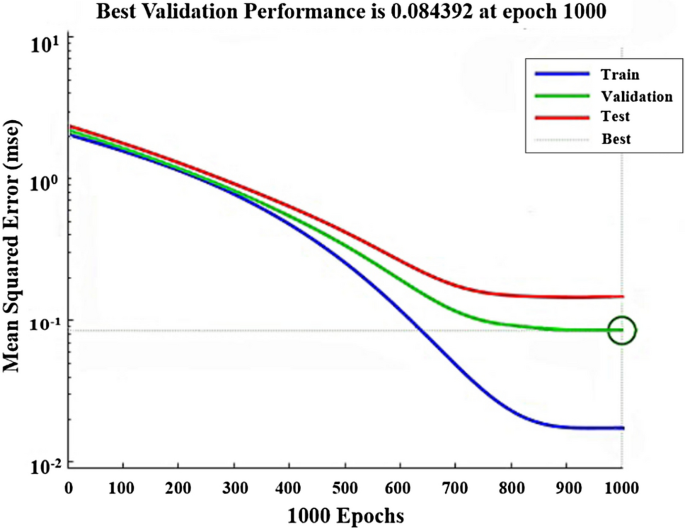
Performance of the single-point stagnant water prediction model in training and testing
Fig. 12 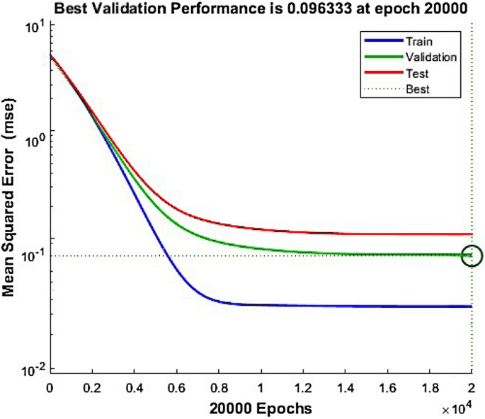
Performance of the spatial stagnant water prediction model in training and testing
-
(5)
Model prediction
In the model prediction process, a real short-duration rainstorm event that occurred on 26 May 2019 was selected as the rainfall scenario, its rainfall time series was converted into a training database format, and the prediction model that had been trained and adjusted was used as input. The water accumulation depth of each high-risk point in this scenario was predicted in time and space, and its error was calculated. The rainfall and stagnant water data come from the Tianjin Meteorological Research Institute.


3.5 Result Analysis
Based on the previous analyses and calculations, under the 26 May 2019 rainstorm scenario, the coupled neural network-numerical simulation of the water depth spatiotemporal prediction model was used to predict the water depth of the corresponding high-risk points in the drainage area. The PCSWMM-based urban flood simulation was carried out with the 26 May rainstorm as the model boundary, and the inundation information of the seven high-risk points was extracted, as shown in Table 5. Compared with the actual results, the predicted water depth is in the range of 8.86–27.12 cm, the actual water depth is 6.9–27.1 cm, and the average difference is 2.67 cm. NSE = 0.88, RMSE = 2.49, R2=0.78, PE = 0.00074, and the fitting accuracy meets the requirements. In summary, the spatiotemporal prediction model of stagnant water based on neural network-numerical simulation has good reliability.
To verify the timeliness of the neural network-numerical simulation water accumulation rapid prediction model proposed in this study and determine whether it can meet the urban flood emergency management requirements, after predicting the accumulation of water at high-risk points in the study area, the same scenario simulation based on the PCSWMM hydrological and hydrodynamic model was performed using the same computer. The time required to run the simulations of the two models are shown in Table 6. For a rainfall event that lasts for 2 hours, the water accumulation prediction based on the physical model required approximately 15 minutes, while the rapid prediction model required approximately 20 seconds. Even if the expansion of the training database will increase its prediction time, its speed is still much higher than that of the physical model, and it can meet the requirements of urban flood emergency management, which has certain practical application value.
4 Discussion
In practical applications, the developed model can be matched with several designed rainstorm patterns, according to the actual rainfall characteristics, and the most suitable rain pattern is selected for time-history allocation to obtain the actual rainfall process. Inputting the prediction model of the maximum water depth in time and space constructed in this study can obtain the inundation situation of each spatial point under rainfall to take the corresponding flood prevention measures. On the one hand, based on the upcoming rainfall forecast data, we can substitute the rainfall process data for the next 3 hours into the model for calculation to quickly predict stagnant water and provide it to emergency management departments to inform response. On the other hand, according to the real-time monitoring of the rainfall process (greater than 10 min), we can divide the rainfall into 10 equal parts and continuously substitute it into the model to quickly calculate and predict the accumulation of water. At this time, the calculation speed can be synchronized with the rainfall. For example, if a rainfall data monitoring value is obtained in 1 minute, we can obtain the rainfall process in 10 minutes and input it into the model after matching the rain pattern to obtain the waterlogging situation of each high-risk point. A longer monitoring time can also continue to input data into the model to continuously output the flooding situation to achieve real-time prediction. Emergency management departments can take quicker measures against floods caused by heavy rain based on real-time output data to minimize disaster losses. In addition, because this model can output the accumulation of water at multiple points according to rainfall and has high accuracy, in actual management, only one of the high-risk points in the study area needs to be added with a monitoring instrument for the accumulation of water.
In this study, our rainfall database has only 35 data samples composed of 5 rain patterns and 7 return periods, which inevitably affects the prediction accuracy. Therefore, in order to improve the prediction accuracy, more rain patterns can be added in future applications to obtain more sample data, so that the real-time prediction results of floods are more accurate.
5 Conclusion
Aiming at the prediction of accumulated water in flood emergencies in an urban area, this study proposed a prediction model of the maximum water depth in time and space employing a neural network-numerical simulation model on the basis of coupling a two-dimensional hydrological and hydrodynamic model and a statistical analysis model. A rainfall-accumulating water database and a spatial point water depth prediction database were established. We used the nonlinear approximation ability and dynamic memory ability of the Elman neural network to learn and memorize the mapping relationship from the input rainfall scenario to the maximum water depth of the output, and the single point water depth of the input to the spatial accumulation of water in the output. A quick prediction model of stagnant water was constructed, and the trend of stagnant water change was predicted by the iterative forecasting method. The results show that the NSE of the stagnant water prediction model based on neural network-spatial coordinates is 0.876, which has good reliability, and the prediction speed of this model is much higher than that of the physical model.
The results of this study can instantly predict the submerged water depth of the corresponding risk point in the city based on rainstorm information, which has the advantages of a higher accuracy, a faster response speed, and a more accurate prediction. It has great application value in coastal city flood prevention, disaster mitigation, and smart city flood emergency management. It has certain theoretical and practical significance for optimizing the arrangement of water accumulation detection points in the study area and for flood emergency prevention and disaster mitigation. It can provide a certain scientific basis for guiding the allocation of urban resources and supporting the design of emergency plans by the relevant government departments. This model considers various commonly designed rain patterns, but due to data limitations, the actual rainfall and waterlogging data were not added to the database for training. Therefore, although the performance of the prediction model is satisfactory, its accuracy can be improved further after collecting enough data.
References
Ahiablame, L., and R. Shakya. 2016. Modeling flood reduction effects of low impact development at a watershed scale. Journal of Environmental Management 171: 81–91.
Banik, B.K., L. Alfonso, A.S. Torres, A. Mynett, C.D. Cristo, and A. Leopardi. 2015. Optimal placement of water quality monitoring stations in sewer systems: An information theory approach. Procedia Engineering 119: 1308–1317.
Beck, J. 2016. Comparison of three methodologies for Quasi-2D river flood modeling with SWMM5. Journal of Water Management Modeling. https://doi.org/10.14796/JWMM.C402.
Bowes, B.D., J.M. Sadler, M.M. Morsy, M. Behl, and J.L. Goodall. 2019. Forecasting groundwater table in a flood prone coastal city with long short-term memory and recurrent neural networks. Water 11(5): Article 1098.
Guo, Z., J.P. Leitao, N.E. Simoes, and V. Moosavi. 2020. Data-driven flood emulation: Speeding up urban flood predictions by deep convolutional neural networks. Journal of Flood Risk Management 14(1): Article e12684.
Hammond, M.J., A.S. Chen, S. Djordjevic, D. Butler, and O. Mark. 2015. Urban flood impact assessment: A state-of-the-art review. Urban Water Journal 12(1–2): 14–29.
Hou, J.M., N. Zhou, G. Chen, M. Huang, and G. Bai. 2021. Rapid forecasting of urban flood inundation using multiple machine learning models. Natural Hazards. https://doi.org/10.1007/s11069-021-04782-x.
Huang, G.R., X. Wang, and W. Huang. 2017. Simulation of rainstorm water logging in urban area based on InfoWorks ICM Model. Water Resources and Power 35(2): 66–70; 60 (in Chinese).
Huang, J.H., C. Wang, and Z.H. Fan. 2020. Evolution of design rainfall pattern in Tianjin. Water Resources Protection 36(1): 38–43 (in Chinese).
Huff, F.A. 1967. Time distributions of heavy rainstorms in Illinois. Water Resources Research 3(4): 1007–1019.
Kabir, S., S. Patidar, X.L. Xia, Q.H. Liang, J. Neal, and G. Pender. 2020. A deep convolutional neural network model for rapid prediction of fluvial flood inundation. Journal of Hydrology 590: 2335–2356.
Keifer, C.J., and H.H. Chu. 1957. Synthetic storm pattern for drainage design. Journal of Hydraulics Division 83: 1–25.
Kim, H.I., and K.Y. Han. 2020. Data-driven approach for the rapid simulation of urban flood prediction. KSCE Journal of Civil Engineering 24: 1932–1943.
Kim, H.I., H.J. Keum, and K.Y. Han. 2019. Real-time urban inundation prediction combining hydraulic and probabilistic methods. Water 11(2): Article 293.
Krupka, M. 2009. A rapid inundation flood cell model for flood risk analysis. Edinburgh, UK: Heriot-Watt University.
Lee, J.Y., C. Choi, D. Kang, B.S. Kim, and T.W. Kim. 2020. Estimating design floods at ungauged watersheds in South Korea using machine learning models. Water 12(11): Article 3022.
Lee, J., and B. Kim. 2021. Scenario-based real-time flood prediction with logistic regression. Water 13(9): Article 1191.
Leitao, J.P., N.E. Simoes, C. Maksimovic, F. Ferreira, D. Prodanovic, J.S. Matos, and A. Sa Marques. 2010. Real-time forecasting urban drainage models: Full or simplified networks?. Water Science and Technology 62(9): 2106–2114.
Li, X.H., and P. Willems. 2020. A hybrid model for fast and probabilistic urban pluvial flood prediction. Water Resources Research 56(6): Article e2019WR025128.
Liu, Y., S. Zhang, L. Liu, X. Wang, and H. Huang. 2015. Research on urban flood simulation: A review from the smart city perspective. Progress in Geography 34(4): 494–504.
María, T.C., G. Jorge, and E. Cristián. 2020. Forecasting flood hazards in real time: A surrogate model for hydrometeorological events in an Andean watershed. Natural Hazards and Earth System Sciences 20(12): 3261–3277.
May, W. 2008. Potential future changes in the characteristics of daily precipitation in Europe simulated by the HIRHAM regional climate model. Climate Dynamics 30(6): 581–603.
Meng, L., H. Wu, J.X. Wang, and M. Lei. 2009. Application of Elman neural network to width spread prediction in Medium Plate Mill. In Proceedings of the 2009 International Conference on Measuring Technology and Mechatronics Automation, 11–12 April 2009, Zhangjiajie, China:187–190.
Moulin, L., E. Gaume, and C. Obled. 2009. Uncertainties on mean areal precipitation: Assessment and impact on streamflow simulations. Hydrology and Earth System Sciences 13(2): 99–114.
Mounce, S.R., W. Shepherd, G. Sailor, J. Shucksmith, and A.J. Saul. 2014. Predicting combined sewer overflows chamber depth using artificial neural networks with rainfall radar data. Water Science and Technology 69(6): 1326–1333.
Nash, J.E., and J.V. Sutcliffe. 1970. River flow forecasting through conceptual models part I – A discussion of principles. Journal of Hydrology 10(3): 282–290.
Rjeily, Y.A., O. Abbas, M. Sadek, I. Shahrour, and F.H. Chehade. 2017. Flood forecasting within urban drainage systems using NARX neural network. Water Science and Technology 76(9): 2401–2412.
Santhi, C., J.G. Arnold, J.R. Williams, W.A. Dugas, R. Srinivasan, and L.M. Hauck. 2010. Validation of the SWAT model on a large river basin with point and nonpoint sources. Journal of the American Water Resources Association 37(5): 1169–1188.
She, L., and X.Y. You. 2019. A dynamic flow forecast model for urban drainage using the coupled artificial neural network. Water Resources Management 33(9): 3143–3153.
Wan, X., Q. Yang, P. Jiang, and P. Zhong. 2019. A hybrid model for real-time probabilistic flood forecasting using Elman neural network with heterogeneity of error distributions. Water Resources Management 33(11): 4027–4050.
Wei, M., L. She, and X.Y. You. 2020. Establishment of urban waterlogging pre-warning system based on coupling RBF-NARX neural networks. Water Science and Technology 82(9): 1921–1931.
Wu, H.C., and G.R. Huang. 2016. Risk assessment of urban waterlogging based on PCSWMM model. Water Resources Protection 32(05): 11–16 (in Chinese).
Wu, Z., Y. Zhou, and H. Wang. 2020. Real-time prediction of the water accumulation process of urban stormy accumulation points based on deep learning. IEEE Access 8: 151938–151951.
Yan, J., J.M. Jin, F.R. Chen, G. Yu, H.L. Yin, and W.J. Wang. 2018. Urban flash flood forecast using support vector machine and numerical simulation. Journal of Hydroinformatics 20(1): 221–231.
Yin, J., M. Ye, Z. Yin, and S. Xu. 2015. A review of advances in urban flood risk analysis over China. Stochastic Environmental Research and Risk Assessment 29: 1063–1070.
Zanchetta, A.D.L., and P. Coulibaly. 2020. Recent advances in real-time pluvial flash flood forecasting. Water 12(2): Article 570.
Zeng, Z., Z. Wang, X. Wu, C. Lai, and X. Chen. 2017. Rainstorm waterlogging simulations based on SWMM and LISFLOOD models. Journal of Hydroelectric Engineering 36(5): 68–77 (in Chinese).
Zhang, M., L.F. Zhao, and X. Quan. 2019. Application of Echo State Network in the prediction of water level at urban waterlogging points. China Rural Water and Hydropower (6): 56–59; 65 (in Chinese).
Zhang, S., and B. Pan. 2014. An urban storm-inundation simulation method based on GIS. Journal of Hydrology 517(5): 260–268.
Zheng, S.S., Q. Wan, and M.Y. Jia. 2014. Short-term forecasting of waterlogging at urban storm-waterlogging monitoring sites based on STARMA model. Progress in Geography 33(7): 949–957 (in Chinese).
Acknowledgments
This research was supported by the Water Pollution Control and Treatment of Major National Science and Technology Project of China (2017ZX07106001), the National Natural Science Foundation of China (51509179), and the Tianjin Natural Science Foundation (20JCQNJC01540). The authors acknowledge the assistance of the anonymous reviewers.
Author information
Authors and Affiliations
Corresponding author
Rights and permissions
Open Access This article is licensed under a Creative Commons Attribution 4.0 International License, which permits use, sharing, adaptation, distribution and reproduction in any medium or format, as long as you give appropriate credit to the original author(s) and the source, provide a link to the Creative Commons licence, and indicate if changes were made. The images or other third party material in this article are included in the article's Creative Commons licence, unless indicated otherwise in a credit line to the material. If material is not included in the article's Creative Commons licence and your intended use is not permitted by statutory regulation or exceeds the permitted use, you will need to obtain permission directly from the copyright holder. To view a copy of this licence, visit http://creativecommons.org/licenses/by/4.0/.
About this article

Cite this article
Yan, X., Xu, K., Feng, W. et al. A Rapid Prediction Model of Urban Flood Inundation in a High-Risk Area Coupling Machine Learning and Numerical Simulation Approaches. Int J Disaster Risk Sci 12, 903–918 (2021). https://doi.org/10.1007/s13753-021-00384-0
Accepted:
Published:
Issue Date:
DOI: https://doi.org/10.1007/s13753-021-00384-0