Optimal selection of contracts and work shifts in multi-skill call centers

Abstract

This paper deals with the problem of finding the most suitable contracts to be used when hiring the operators of a call center and deciding their optimal working schedule, to optimize the trade-off between the service level provided to the customers and the cost of the personnel. In a previous paper (Cordone et al. 2011), we proposed a heuristic method to quickly build an integer solution from the solution of the continuous relaxation of an integer linear programming model. In this paper, we generalize that model to take into account a much wider class of working contracts, allowing heterogeneous shift patterns, as well as legal constraints related to continuously active working environments. Since our original rounding heuristic cannot be extended to the new model, due to its huge size and to the involved correlations between different sets of integer variables, we introduce a more sophisticated heuristic based on decomposition and on a multi-level iterative structure. We compare the results of this heuristic with those of a Greedy Randomized Adaptive Search Procedure, both on real-world instances and on realistic random instances.

Introduction

The inherent complexity of call center design and management and the growing size of the organizations involved in customer operations strongly call for precise optimization techniques that allow a satisfactory trade-off between the level of service provided to the customers and the cost of providing it. On one hand, the personnel costs could largely exceed the needs; on the other hand, the customers could receive a poor level of service, in terms of timely and satisfactory responses. This motivates the development of decision support systems, including tools to forecast, control and improve key performance indicators. The aim is to optimize the relation between the volume of the demand, the resources deployed, and the quality of service.

Workforce management in call centers is a paradigmatic example of service optimization, illustrating the fundamental role of operations research in service science, since a large amount of the call center operational costs are related to its personnel. For an extensive treatment of call center management problems and techniques, we refer to (Gans et al. 2003). Multi-skill call centers, in particular, require not only to define the appropriate number of operators, but also to determine in detail the appropriate mix of skills provided at each time of each day during a given time horizon. To model this situation, each operator is characterized by a profile, i.e. a set of skills. In the ideal case, all operators should have all skills, but this would be too costly. However, a careful mix and distribution of operators with a limited number of skills are enough to provide significant benefits to the overall performance at a limited training cost. This has been shown, under mild assumptions, even in the case of operators with as few as two skills (Wallace and Whitt 2005). In practice, typical examples of skills are the ability to speak a certain foreign language or basic knowledge on particular software packages for which the call center provides assistance. Since different customers require different combinations of skills and no operator usually has all skills, one information of importance to a call center management team is what combinations of skills are more beneficial, and consequently whether it would be profitable to train operators to acquire certain additional skills.

Call centers must guarantee at any time the presence of a suitable number of operators and a suitable amount of skills according to the forecasted level of demand. This problem is usually referred to as the staffing problem. In mono-skill services, where the operators run a single type of activity and the volume of calls is very high and well-predictable, queuing theory techniques are enough to provide a reliable estimate of the number of operators needed. The forecast of the demand can be refined to take into account the granularity of the time periods considered, as well as end-of-the-day and peak-hours effects and other details; see for instance Green et al. (2007). An introduction to the staffing problem with a detailed survey can be found in Aksin et al. (2007). In multi-skill call centers, where the operations are more complex, the operators cannot be considered interchangeable any more, because each of them has distinctive skills. Moreover, a suitable mix of complementary skills must be available in the call center at any time of the day. In these cases, the simplifying assumptions about stationary conditions required by queuing theory typically lead to overestimates or underestimates of the number of required operators, and hence to cost inefficiency or performance degradation. Then, simulation and analytical techniques, often used as complementary approaches, can be applied to the staffing problem.

The scientific literature is rich with contributions on statistical and simulation models of incoming calls (Channouf et al. 2007) and consequent phenomena of waiting queues, abandoned calls and call transfers (Avramidis et al. 2009), which allow the level of required capacity to be estimated. Once this has been decided, the next problem is to define suitable work shifts and to assign operators to them, to meet those requirements. While doing that, it is also necessary to consider a significant number of detailed constraints related to labor contracts. The literature on staffing often neglects most of these constraints. All these issues complicate significantly the relation between the decision variables (number and type of labor contracts, operator assignment, day-by-day work shifts) and the effects produced (costs and level of service obtained during each day) (Avramidis et al. 2007; Chan et al. 2007). Most of the few approaches which take into account all the features mentioned above work in two phases: the former defines the optimal set of operators, the latter computes the optimal schedule for the given set of operators (Pot 2006; Pisacane et al. 2006). Unfortunately, the independent solution of the shift rostering problem and the shift scheduling problem is a source of inefficiency, as pointed out in the comprehensive review paper by Aksin et al. (2007), which collects contributions combining simulation, queuing theory, mathematical programming and heuristics.

Our previous study ( Cordone et al. 2011) provided an integrated solution for the two different, but related, sub-problems of defining (1) the optimal mix of labor contracts to stipulate with the operators and (2) the optimal schedule of work shifts of the operators. This paper aims at extending the range of application to a wider set of possible contracts, to take into account the increase in the number of allowed contract types in modern call centers. We also consider additional constraints related to the correct assignment of work shifts to the operators. For example, we avoid assigning two work shifts too close to each other, which can easily happen in call centers whose activity extends continuously 24 h a day. We also extend the time horizon over which the model is solved to take into account some sort of seasonality. The model obtained is significantly harder compared to that studied in  Cordone et al. (2011). To cope with the increased complexity of the new problem, we introduce a heuristic which exploits the mathematical programming formulation of the problem to decompose it into sub-problems, and derive from the continuous relaxation of each sub-problem an integer solution through a multi-level iterative rounding approach. For comparison purposes, this work also proposes a Greedy Randomized Adaptive Search Procedure (GRASP) to build solutions in a more straightforward manner Feo and Resende (1989). Finally, we show that, on a set of real-world and of realistic instances, the two methods provide solutions of comparable quality. We do not address here the rostering problem, that is the assignment of specific individual operators to work shifts, because in our case all operators with the same skill profile and labor contract are indistinguishable, and no personal preferences are taken into account at this level of detail.

Section 2 defines the integrated problem and provides its integer linear programming (ILP) formulation. Sections 3 and 4, respectively, describe the rounding heuristic adopted to attack the huge ILP formulation, and the alternative GRASP heuristic. Section 5 presents computational results on real-world as well as randomly generated instances.

Problem description

The problem we consider here is to determine how many operators with a given set of skills should be hired with each available contract form and how their work shifts should be organized during a given time horizon, to meet as tightly as possible a forecasted demand profile for each set of skills. Since the problem considered is extremely complex and exhibits several levels of detail, we structure its presentation in subsequent steps, starting from the more general level, with the objective function, the decision variables directly influencing it and the main constraints linking them. The following subsections will focus on more specific aspects, concerning the relation between contracts, shifts and lunch breaks, the balance between different contract types, and the distribution of shifts over time (weekly shift patterns, synchronization along the days of a week, minimum distance between consecutive shifts, rest periods).

General framework

Data (1). A profile is defined as a set of particular skills used to classify the operators:

• $\mathcal {G}$ is the set of all possible operator profiles.

Operators with the same profile are considered undistinguishable. No personal preferences or personal data are taken into account.

The time horizon is defined as follows:

• $\mathcal {O}$ is a sequence of consecutive weeks;

• each week is composed of a sequence $\mathcal {D}= \{1,\ldots ,7\}$ of 7 days;

• each day is composed of a sequence $\mathcal {T}= \{ 1,\ldots ,|\mathcal {T}| \}$ of time slices of given duration $L$, extending over 24 h.

In our experiments, we used $|\mathcal {T}| = 48$ time slices of $L = 30\,\mathrm{min}$.

The working schedule must be planned over the time horizon to meet an estimate of the skills demanded in each time slice:

• $f_{godt}$ is the number of operators required for each profile $g \in \mathcal {G}$, week $o \in \mathcal {O}$, day $d \in \mathcal {D}$ and time slice $t \in \mathcal {T}$.

This forecast describes the expected seasonality of the demand and is assumed to have been obtained in a previous analysis (see  Cordone et al. 2011).

The estimated demand can be missed, in excess or in defect, but the difference between the achieved and the required values must be made as small as possible.

Variables (1). We define the following decision variables for each profile $g \in \mathcal {G}$, week $o \in \mathcal {O}$, day $d \in \mathcal {D}$ and time slice $t \in \mathcal {T}$:

• $y_{godt}$, integer, is the number of operators at work;

• $w^{+}_{godt}, w^{-}_{godt} \ge 0$ are the surplus and deficit of operators with respect to the forecasted demand $f_{godt}$.

Objective function. The objective function, to be minimized, is a weighted combination of over- and under-staffing:

$$\begin{aligned} \min \sum \limits _{g \in \mathcal {G}} \sum \limits _{o \in \mathcal {O}} \sum _{d \in \mathcal {D}} \sum _{t \in \mathcal {T}} \left[ \alpha w^+_{godt} + (1-\alpha ) w^-_{godt} \right] \end{aligned}$$

(1)

where parameter $\alpha \in \left[ 0,1 \right]$ weighs the relative importance of the surplus and the deficit of operators, and consequently determines the trade-off between the personnel cost and the level of service.

Constraints (1). The variables are linked by the following relations:

$$\begin{aligned} w^+_{godt}&\ge y_{godt} - f_{godt}&o \in \mathcal {O}, g \in \mathcal {G}, d \in \mathcal {D}, t \in \mathcal {T}\end{aligned}$$

(2)

$$\begin{aligned} w^-_{godt}&\ge f_{godt} - y_{godt}&o \in \mathcal {O}, g \in \mathcal {G}, d \in \mathcal {D}, t \in \mathcal {T} \end{aligned}$$

(3)

Data (2). We also denote by

• $\Phi$ the maximum number of operators that can be simultaneously working at any time,

i.e. the number of physically available desks in the call center.

Constraints (2). The model includes the following capacity constraint:

$$\begin{aligned} \sum _{g \in \mathcal {G}} y_{godt} \le \Phi \qquad \qquad o \in \mathcal {O}, d \in \mathcal {D}, t \in \mathcal {T} \end{aligned}$$

(4)

Contracts, shifts and patterns

The operators of multi-skill call centers usually have a wide variety of different labor contracts. The mix of contracts adopted by a call center service has a relevant influence on the possibility to track the forecasted demand of different skill profiles over time, because the contracts determine not only the total amount of work hours of each operator during the time horizon, but also their detailed distribution. The patterns followed by work shifts can be quite sophisticated and sometimes they yield complex situations in which the same operator performs different shifts in different weeks.

Another relevant issue is the distribution of lunch breaks, which create a noticeable reduction in the number of available operators. Neglecting it would introduce a systematic error in the evaluation of the objective function.

To account for these details, it is necessary to introduce additional data, decision variables and constraints.

Data (3). We define the following two sets:

• $\mathcal {M}$ is the set of all possible contracts;

• $\mathcal {H}$ is the set of all possible work shifts.

Each work shift is characterized by its time length:

• $\delta _h$ is the number of consecutive time slices of length $L$ taken by shift $h \in \mathcal {H}$.

Conventionally, shift $h=0$ models a day of rest, and has $\delta _{0} = 0$.

For each contract $m \in \mathcal {M}$ we also define:

• $\mathcal {W}_m$ as the set of weekly shift patterns for contract $m \in \mathcal {M}$;

• $N_{mwh}$ as the number of shifts of type $h \in \mathcal {H}$ that must be assigned each week to a worker with contract $m \in \mathcal {M}$ following pattern $w \in \mathcal {W}_{m}$.

A shift pattern $w$ does not determine the specific days and time slices in which the work shifts must be performed, but constrains their overall number of occurrences:

• set $\mathcal {H}_{mwd}$ collects the work shifts available for an operator with contract $m \in \mathcal {M}$ following weekly pattern $w \in \mathcal {W}_{m}$ in day $d \in \mathcal {D}$;

• set $\mathcal {T}_{mwdh}$ collects the time slices in which an operator with contract $m \in \mathcal {M}$ who follows the weekly pattern $w \in \mathcal {W}_{m}$ can start shift $h \in \mathcal {H}_{mwd}$ in day $d \in \mathcal {D}$;

• $s_{mw}$ is the number of weeks during the time horizon $\mathcal {O}$ for which an operator with contract $m \in \mathcal {M}$ must follow pattern $w \in \mathcal {W}_{m}$.

Example 1

Let contract $m$ admit two weekly shift patterns $\mathcal {W}_m = \{ w_{1},w_{2} \}$:

• pattern $w_{1}$ includes a shift of 8 hours (8 h) and a rest shift (0), that must be performed, respectively, five times ($N_{mw_{1}\,\mathrm{8\,h}} = 5$) and two times ($N_{mw_{1}\,0} = 2$); Saturday and Sunday must be days of rest ($\mathcal {H}_{mw_{1}\,6} = \mathcal {H}_{mw_{1}\,7} = \{ 0 \}$);

• pattern $w_{2}$ includes four shifts (0,4 h,6 h,8 h), $\mathcal {H}_{m2}=\{0,4\,\mathrm{h},6\,\mathrm{h},8\,\mathrm{h}\}$, respectively, with $N_{mw_{2}\,0}=2$, $N_{mw_{2}\,4\,\mathrm{h}}=2$, $N_{mw_{2}\,6\,\mathrm{h}}=1$ and $N_{mw_{2}\,8\,\mathrm{h}}=2$ repetitions per week; on Wednesday the 4-h shift is mandatory ($\mathcal {H}_{mw_{2}\,3}=\{4\,\mathrm{h}\}$).

Assuming a 4-week time horizon $\mathcal {O}= \{1,2,3,4\}$, with 2 weeks for each shift pattern ($s_{mw_{1}} = 2$ and $s_{mw_{2}} = 2$), an example of feasible solution could be:

Week	Pattern	Day
$o$	$w$	Mon	Tue	Wed	Thu	Fri	Sat	Sun
1	$w_{1}$	8 h	8 h	8 h	8 h	8 h	0	0
2	$w_{2}$	0	6 h	4 h	4 h	0	4 h	8 h
3	$w_{2}$	6 h	8 h	4 h	8 h	0	0	4 h
4	$w_{1}$	8 h	8 h	8 h	8 h	8 h	0	0

Notice that in pattern $w_{1}$ the assignment of shifts to days is completely fixed, whereas pattern $w_{2}$ allows some flexibility; in fact, the distribution of shifts along weeks $o = 2$ and $o = 3$ is different, even though they both follow pattern $w_{2}$.

For a subset $\mathcal {M}^{\mathrm {fix}} \subseteq \mathcal {M}$ of contracts,$\mathcal {W}_{m}$ is associated with a given fixed sequence of $\omega _{m}$ weekly shift patterns which must be followed exactly. For the sake of simplicity, the operators with each of those contracts are divided into $|\mathcal {O}|$ equal groups which follow circular shifts of the fixed sequence.

Example 2

Let contract $m$ admit three weekly shift patterns $\mathcal {W}_m = \{ w_{1},w_{2},w_{3} \}$ with $s_{mw_{1}} = 1$, $s_{mw_{2}} = 2$ and $s_{mw_{3}} = 1$, associated with the sequence $\omega _{m} = \left( w_{1},w_{2},w_{3},w_{2} \right)$. The time horizon spans over four weeks ($\mathcal {O}= \{1,\ldots ,4\}$).

An example of feasible solution could be the following. Notice how the sequence $\omega _m$ is circularly shifted on $|\mathcal {O}|$ different groups of operators, to achieve a balanced distribution.

Week	Operator group
$o$	1	2	3	4
1	$w_{1}$	$w_{2}$	$w_{3}$	$w_{2}$
2	$w_{2}$	$w_{1}$	$w_{2}$	$w_{3}$
3	$w_{3}$	$w_{2}$	$w_{1}$	$w_{2}$
4	$w_{2}$	$w_{3}$	$w_{2}$	$w_{1}$

All these characteristics define a very broad range of contract types, full-time or part-time, with or without fixed resting days, with an explosive number of shift combinations. Further refinements in the description of contracts will be given in the following sections.

Variable (3). To describe the distribution of shifts over time, we introduce the following variables:

• $z_{gmwodht}$, integer, is the number of operators with profile $g \in \mathcal {G}$ and contract $m \in \mathcal {M}$ who follow pattern $w \in \mathcal {W}_m$ during week $o \in \mathcal {O}$ and in day $d \in \mathcal {D}$ perform working shift $h \in \mathcal {H}_{mwd}$ starting at time slice $t \in \mathcal {T}_{mwdh}$;

Notice that variables $z$ give a very fine-grained description of the solution:a deeper detail would amount to considering each operator individually. These variables are set to zero for all forbidden combinations of the indices, i.e., when $w \notin \mathcal {W}_m$ or $h \notin \mathcal {H}_{mwd}$ or $t \notin \mathcal {T}_{mwdh}$.

Constraints (3). We are given the following threshold:

• $v_{mt}$ is the maximum allowed number of operators with contract $m \in \mathcal {M}$ who can start working at time $t \in \mathcal {T}$ in any day of the time horizon.

This is to ensure that the operators with the same contract are distributed among different times of the day. The number of operators simultaneously starting a shift is hence limited by the following constraint:

$$\begin{aligned} \sum _{g \in \mathcal {G}} \sum _{w \in \mathcal {W}_{m}} \sum _{h \in \mathcal {H}_{mwd}} z_{gmwodht} \le v_{mt} \quad m \in \mathcal {M}, o \in O, d \in \mathcal {D}, t \in \mathcal {T} \end{aligned}$$

(5)

Lunch breaks

Variables (4). To describe the distribution of lunch breaks over time, we introduce the following variables:

• $\psi _{gmodht}$, integer, is the number of operators with profile $g \in \mathcal {G}$ and contract $m \in \mathcal {M}$, who in week $o \in \mathcal {O}$ and day $d \in D$ perform shift $h \in \mathcal {H}$ and leave for lunch in time slice $t \in \mathcal {T}$.

Data (4). We denote by

• $\pi _{mh}$ the duration of lunch breaks for operators with contract $m \in \mathcal {M}$ performing shift $h \in \mathcal {H}$,

• $\eta _{mht}$ and $\mu _{mht}$ the minimum distance from the beginning and from the end of the shift which an operator must respect when leaving for lunch, depending on the contract $m \in \mathcal {M}$, the shift $h \in \mathcal {H}$ and the starting time slice $t \in \mathcal {T}$.

Each of these time lengths is expressed as a number of consecutive time slices.

Constraints (4). First of all, Eq. (6) forces the number of operators having a lunch break on a specific day $d$ (left-hand side) to be equal to the number of shifts that require a lunch break on the same day (right-hand side). Notice that the latter term sums shifts starting early enough on day $d$ and shifts starting late enough on the previous day, $d-1$. To guarantee the minimum distance of a lunch break from the beginning of the shift, the left-hand side of Constraint (7) enumerates the lunch breaks starting no later than time $t$, while the right-hand side enumerates the shifts for which the lunch break can start no later than $t$: the inequality guarantees that no lunch break starts too early. Analogously, the left-hand side of Constraint (8) enumerates the lunch breaks starting no sooner than time $t$, while the right-hand side enumerates the shifts for which the lunch break can end no sooner than $t$: the inequality guarantees that no lunch break starts too late. The use of inequalities to impose the correct distribution of lunch breaks could allow to introduce less breaks than shifts, but this is forbidden by Eq. (6).

$$\begin{aligned} \sum \limits _{t =1}^{|\mathcal {T}|} \psi _{gmodht}&= \sum \limits _{w \in \mathcal {W}_{m}} \left( \sum \limits _{t = 1}^{|\mathcal {T}|-\eta _{mht}+1} z_{gmwodht} + \sum \limits _{t = |\mathcal {T}|-\eta _{mht}+2}^{|\mathcal {T}|} z_{gmwo\,d-1\,ht} \right) \nonumber \\&\quad g \in \mathcal {G}, \left( m,h \right) \in \mathcal {M}\times \mathcal {H}:\ \pi _{mh} > 0,\ o \in \mathcal {O},\ d \in \mathcal {D}\end{aligned}$$

(6)

$$\begin{aligned} \sum \limits _{\tau = 1}^{t} \psi _{gmodh\tau }&\le \sum \limits _{w \in \mathcal {W}_{m}} \left( \sum \limits _{\tau =1}^{t-\eta _{mh\tau }+1} z_{gmwodh\tau } + \sum \limits _{\tau = |\mathcal {T}|-\delta _h+\mu _{mh\tau }+1}^{t-\eta _{mh\tau }+1+|\mathcal {T}|} z_{gmwo\,d-1\,h\tau } \right) \nonumber \\&\quad g \in \mathcal {G}, \left( m,h \right) \in \mathcal {M}\times \mathcal {H}:\ \pi _{mh} > 0,\ o \in \mathcal {O},\ d \in \mathcal {D},\ t \in \mathcal {T}\qquad \end{aligned}$$

(7)

$$\begin{aligned} \sum \limits _{\tau = t}^{|\mathcal {T}|} \psi _{gmodh\tau }&\le \sum _{w \in \mathcal {W}_{m}} \left( \sum \limits _{\tau = t-\delta _h+\mu _{mh\tau }}^{|\mathcal {T}|} z_{gmwodh\tau } + \sum \limits _{\tau = t-\delta _h+\mu _{mh\tau }+| \mathcal {T}|}^{|\mathcal {T}|} z_{gmwo\,d-1\,h\tau } \right) \nonumber \\&\quad g \in \mathcal {G}, \left( m,h \right) \in \mathcal {M}\times \mathcal {H}:\ \pi _{mh} > 0,\ o \in \mathcal {O},\ d \in \mathcal {D},\ t \in \mathcal {T} \end{aligned}$$

(8)

The $y$ variables, which measure the service offer, are directly related to the $z$ and $\psi$ variables:

$$\begin{aligned} y_{godt}&= \sum _{m \in \mathcal {M}} \sum _{h \in \mathcal {H}} \left( \sum _{w \in \mathcal {W}_m} \sum _{\tau = t-\delta _h+1}^{t} z_{gmwodh\tau } - \sum _{\tau = t-\pi _{mh}+1}^{t} \psi _{gmodh\tau } \right) \nonumber \\&\quad g \in \mathcal {G}, o \in \mathcal {O}, d \in \mathcal {D}, t \in \mathcal {T} \end{aligned}$$

(9)

Notice that, when $t-\delta _h+1 < 0$ or $t-\pi _{mh}+1 < 0$, the negative values of index $\tau$ should be interpreted modulo 24 h, as representing time slices of day $d-1$. If $d = 1$, they represent, modulo 7 days, time slices of week $o-1$. If they point to time slices preceding the current time horizon, one should derive their values from the data on the working shifts assigned in the previous period.

Contract mix

We need to take into account also limitations on the number of operators that can be allocated to each type of contract. In practice, for example, law restrictions can impose a minimum fraction of full-time contracts, so that we may want to limit the amount of part-time contracts to obtain an acceptable balance. Similar limitations can be required by the management.

Data (5). In particular:

• $V^{\max }_{m}$ is the maximum number of operators that can have contract $m \in \mathcal {M}$;

• $u^{\min }_{gm}, u^{\max }_{gm}$ are the minimum and maximum numbers of operators with a given profile $g \in \mathcal {G}$ and contract $m \in \mathcal {M}$.

Variables (5). The balance requirements can be expressed using the fine-grained variables $z$, but to make the model more readable we introduce ad hoc aggregated variables:

• $n_{gmwo}$, integer, is the number of operators with profile $g \in \mathcal {G}$ and contract $m \in \mathcal {M}$ who follow pattern $w \in \mathcal {W}_m$ during week $o \in \mathcal {O}$;

• $x_{gm}$, integer, is the number of operators with profile $g \in \mathcal {G}$ and contract $m \in \mathcal {M}$.

Constraints (5). The new variables can be directly expressed in terms of the low-level ones:

$$\begin{aligned} n_{gmwo}&= \sum _{h \in \mathcal {H}_{mwd}} \sum _{t \in \mathcal {T}} z_{gmwodht}&g \in \mathcal {G}, m \in \mathcal {M}, o \in \mathcal {O}, d \in \mathcal {D}, w \in \mathcal {W}_m \end{aligned}$$

(10)

$$\begin{aligned} x_{gm}&= \sum _{w \in \mathcal {W}_m} n_{gmwo}&g \in \mathcal {G}, m \in \mathcal {M}, o \in \mathcal {O} \end{aligned}$$

(11)

Notice that in constraints (10) the sum which defines $n_{gmwo}$ assumes the same value for all days $d \in \mathcal {D}$.

The following constraints enforce the correct amount of work shifts for each contract and week pattern, and that the division among the different week types must be coherent over the whole time horizon $\mathcal {O}$:

$$\begin{aligned} \sum _{d \in \mathcal {D}} \sum _{t \in \mathcal {T}} z_{gmwodht}&= N_{mwh} n_{gmwo}&g \in \mathcal {G}, m \in \mathcal {M}, w \in \mathcal {W}_m, o \in \mathcal {O}, h \in \mathcal {H}\end{aligned}$$

(12)

$$\begin{aligned} \sum _{o \in \mathcal {O}} n_{gmwo}&= s_{mw} x_{gm}&g \in \mathcal {G}, m \in \mathcal {M}\setminus \mathcal {M}^{\mathrm {fix}}, w \in \mathcal {W}_m \end{aligned}$$

(13)

$$\begin{aligned} \left| \mathcal {O}\right| n_{gmwo}&= s_{mw} x_{gm}&g \in \mathcal {G}, m \in \mathcal {M}^{\mathrm {fix}}, w \in \mathcal {W}_m, o \in \mathcal {O} \end{aligned}$$

(14)

Notice that the last constraint requires the operators following the sequence associated with contract $m$ to be divided evenly among the $|\mathcal {O}|$ possible circular shifts. In general, this should be slightly relaxed to avoid conflicts with the integrality requirement. However, both the rounding method, which starts from the continuous relaxation of the model, and the GRASP heuristic are able to cope with such an approximation.

The balance between different contracts is imposed constraining the $x$ variables as follows:

$$\begin{aligned} u^{\min }_{gm} \le x_{gm}&\le u^{\max }_{gm}&g \in \mathcal {G}, m \in \mathcal {M}\end{aligned}$$

(15)

$$\begin{aligned} \sum _{g \in \mathcal {G}} x_{gm}&\le V^{\max }_m&m \in \mathcal {M} \end{aligned}$$

(16)

Labor regulations

We now introduce constraints which ensure that the distribution of the work shifts and rest days over the time horizon respects labor regulations. Since modeling the schedule of each single operator would require an unmanageable level of detail, these constraints are imposed on groups of operators, which are assumed to be interchangeable. Should this assumption lead to infeasibility, we resort to an auxiliary repair routine that is also used to continuously adapt the plan to unpredicted disruptions due to illnesses, holidays, technical problems, and so on. This routine is quite elementary and allows a controlled violation of the less rigid constraints of the model.

The most relevant outcome of the present model is at a strategic level, and consists of the effective distribution of work contracts and profiles among the operators, represented by the values of the $x$ variables, which are not likely to be significantly affected by such minor disruptions. On the other hand, obtaining a detailed schedule, besides being a useful result in itself, gives a reasonable guarantee that the mix of contracts adopted allows to satisfy all constraints with minor modifications while meeting the demand profile.

Data (6). We define:

• $\Theta _{m}$: the maximum number of consecutive working days without a rest according to contract $m \in \mathcal {M}$;

• $\phi$: the minimum required interval between the end of a work shift and the beginning of the next one.

Constraints (6). An operator cannot work more than a certain number of days in a row, without taking a day off:

$$\begin{aligned}&\sum _{w \in \mathcal {W}_m} \sum _{\bar{d} = d-\Theta _m}^{d-1} \sum _{t \in \mathcal {T}} \sum _{h \in \mathcal {H}\setminus \{ 0 \}} z_{gmwo\bar{d}ht} - (\Theta _m-1) x_{gm} \le \sum _{w \in \mathcal {W}_m} \sum _{t \in \mathcal {T}} z_{gmwod0t} \nonumber \\&\quad g \in \mathcal {G}, m \in \mathcal {M}, o \in \mathcal {O}, d \in \mathcal {D} \end{aligned}$$

(17)

Notice that the indices $d-\Theta _m$ and $d-1$, when smaller than 1, should be interpreted modulo 7, propagating the corresponding day over a preceding week. The right-hand side of Constraint (17) indicates the number of operators resting on day $d$; the left-hand side is a lower limit on the number of operators working during the $\Theta _m$ previous days.

The separation between two consecutive work shifts is enforced by requiring the number of operators starting to work during any time interval of length $\phi + \delta _h$ to be never larger that the total number of operators:

$$\begin{aligned} \sum _{w \in \mathcal {W}_m} \sum _{h \in \mathcal {H}\setminus \{0\}} \sum _{\tau = t-\phi -\delta _h+1}^{t} z_{gmwodh\tau } \le x_{gm} \quad g \in \mathcal {G}, m \in \mathcal {M}, d \in \mathcal {D}, t \in \mathcal {T}\qquad \end{aligned}$$

(18)

Once again, index $\tau =t-\phi -\delta _h+1$ should be interpreted modulo 24 h, extending over the previous day, or even the previous week for $d = 1$.

Synchronization

Some particular contracts require the work shifts to be synchronized in different days according to specific rules.

Data (7). Let $\mathcal {S}\subseteq \mathcal {M}$ be the subset of contracts which require the operators to start their shifts at the same time slice in different days of the week. We consider three cases: (1) $\mathcal {S}_1$ includes contracts synchronized over the whole week, (2) $\mathcal {S}_2$ includes contracts synchronized from Monday to Friday, (3) $\mathcal {S}_3$ includes contracts synchronized independently on two different time slices from Monday to Friday and during the weekend.

Variables (7). Correspondingly, we use the following variables, which are slightly more detailed than the $z$ variables, though still avoiding an individual description of the operators:

• $\nu _{gmwot}$, integer, is the number of operators with profile $g \in \mathcal {G}$ and contract $m \in \mathcal {S}_1$ who follow pattern $w \in \mathcal {W}_{m}$ and during all days of week $o \in \mathcal {O}$ start working at time $t \in \mathcal {T}$;

• $\nu ^{h_1h_2}_{gmwot}$, integer, is the number of operators with profile $g \in \mathcal {G}$ and contract $m \in \mathcal {S}_2 \cup \mathcal {S}_3$ who follow pattern $w \in \mathcal {W}_{m}$ and in week $o \in \mathcal {O}$ start working at time $t \in \mathcal {T}$ from Monday to Friday and are assigned shift $h_1$ on Saturday and shift $h_2$ on Sunday;

• $\gamma _{gmwodht}^{h_1h_2}$, integer, is the number of operators with profile $g \in \mathcal {G}$ and contract $m \in \mathcal {S}_2\cup \mathcal {S}_3$ who follow pattern $w \in \mathcal {W}_m$ and in week $o \in \mathcal {O}$ and day $d \in \mathcal {D}$ perform shift $h \in \mathcal {H}$ starting at time slice $t \in \mathcal {T}$, while performing shift $h_1 \in \mathcal {H}$ on Saturday and shift $h_2 \in \mathcal {H}$ on Sunday (therefore, $\gamma _{gmwodht}^{h_1h_2} = 0$ for $d = 6$ and $h \ne h_{1}$ and for $d = 7$ and $h \ne h_{2}$).

Constraints (7). The contracts in $\mathcal {S}_1$ require that each operator starts his shift at the same time slice over the whole week:

$$\begin{aligned} \sum _{d \in \mathcal {D}} z_{gmwodht} = N_{mwh}\, \nu _{gmwot} \quad g \in \mathcal {G}, m \in \mathcal {S}_1, w \in \mathcal {W}_m, o \in \mathcal {O}, h \in \mathcal {H}, t \in \mathcal {T} \end{aligned}$$

(19)

For the other contracts, the $\gamma$ and $z$ variables are related as follows:

$$\begin{aligned} z_{gmwodht} =&\sum _{h_1 \in \mathcal {H}} \sum _{h_2 \in \mathcal {H}} \gamma ^{h_1h_2}_{gmwodht} \nonumber \\&g \in \mathcal {G}, m \in \mathcal {S}_2 \cup \mathcal {S}_3, w \in \mathcal {W}_m, o \in \mathcal {O}, d \in \mathcal {D}, h \in \mathcal {H}_{mwd}, t \in \mathcal {T}\qquad \end{aligned}$$

(20)

The contracts in $\mathcal {S}_2$ and $\mathcal {S}_3$ must be synchronized from Monday to Friday:

$$\begin{aligned} \begin{array}{l@{\quad }l} \sum \limits _{d = 1}^{5} \gamma ^{h_1h_2}_{gmwodht} = \beta _{mwh}^{h_1h_2}\, \nu ^{h_1h_2}_{gmwot} &{}g \in \mathcal {G}, m \in \mathcal {S}_2 \cup \mathcal {S}_3, w \in \mathcal {W}_m, o \in \mathcal {O},\quad \\ &{}t \in \mathcal {T}, h \in \mathcal {H}, h_1 \in \mathcal {H}_{mw6},h_2 \in \mathcal {H}_{mw7} \end{array} \end{aligned}$$

(21)

where

$$\begin{aligned} \beta _{mwh}^{h_1h_2} = \left\{ \begin{array}{l@{\quad }l} N_{mwh} \quad &{}\text { for } h \in \mathcal {H}\setminus \{ h_{1},h_{2} \} \\ N_{mwh}-1\quad &{}\text { for } h \in \{ h_{1},h_{2} \} \text { and } h_1 \ne h_2 \\ N_{mwh}-2\quad &{}\text { for } h = h_1 = h_2 \end{array}\right. \end{aligned}$$

The operators should perform the correct number of shifts during the weekend:

$$\begin{aligned} \sum _{t \in \mathcal {T}} \nu _{gmwot}^{h_1h_2} = \sum _{t \in \mathcal {T}} \gamma _{gmwo\,6h_1t}^{h_1h_2}, \quad h_1 \in \mathcal {H}, h_2 \in \mathcal {H}\end{aligned}$$

(22)

$$\begin{aligned} \sum _{t \in \mathcal {T}} \nu _{gmwot}^{h_1h_2} = \sum _{t \in \mathcal {T}} \gamma _{gmwo\,7h_2t}^{h_1h_2}, \quad h_1 \in \mathcal {H}, h_2 \in \mathcal {H} \end{aligned}$$

(23)

On each day from Monday to Friday, no more than $\nu ^{h_1h_2}_{gmwot}$ operators should work, among those with shifts $(h_1,h_2)$ on the weekend:

$$\begin{aligned}&\sum _{h \in \mathcal {H}_{mwd}} \gamma ^{h_1h_2}_{gmwodht}= \nu ^{h_1h_2}_{gmwot} \nonumber \\&\quad g \in \mathcal {G}, m \in \mathcal {S}_2 \cup \mathcal {S}_3, o \in \mathcal {O}, t \in \mathcal {T}, d \in \left\{ 1,\ldots ,5 \right\} , w \in \mathcal {W}_m \end{aligned}$$

(24)

Another constraint ensures the synchronization of working shifts over the weekend for operators with contracts belonging to $\mathcal {S}_{3}$ and working in shifts $h_1$ and $h_2$ during the week end:

$$\begin{aligned} \gamma ^{h_1h_2}_{gmwo6h_1t} = \gamma ^{h_1h_2}_{gmwo7h_2t}\qquad g \in \mathcal {G}, m \in \mathcal {S}_3, w \in \mathcal {W}_m, o \in \mathcal {O}, t \in \mathcal {T}, h_1,h_2 \in \mathcal {H}_{mwd}\nonumber \\ \end{aligned}$$

(25)

A decomposition and rounding heuristic

For real-world instances, our ILP formulation typically contains millions of variables and constraints. For example, setting a time horizon of $\left| \mathcal {O}\right| = 4$ weeks with time slices of $L = 30\,\mathrm{min}$, the time indices $\left( o,d,t \right)$ range over $\left| \mathcal {O}\right| \cdot \left| \mathcal {D}\right| \cdot \left| \mathcal {T}\right| = 4 \cdot 7 \cdot 48 = 1\,344$ combinations of values. The skill profiles can be as many as $\left| \mathcal {G}\right| = 60$, with a dozen types of contracts ($|\mathcal {M}| = 12$), having a few shift patterns each ($|\mathcal {W}_{m}| \approx 1{-}3$) and $|\mathcal {H}| \approx 7{-}8$ shifts. Consequently, the number of $z$ variables explodes. In many cases, simply generating the model exhausts the memory available on a normal PC, while it is impossible to solve in a reasonable time even its continuous relaxation, not to mention the full problem.

Our approach in  Cordone et al. (2011) concerned a much less detailed and much smaller version of this problem. In that version, the operators followed the same shift pattern week after week during the whole time horizon. As a consequence, the continuous relaxation of the original problem could be solved, and its fractional solution could be easily rounded while respecting all of the constraints. In the version here considered, the fundamental $z$ variables depend also on indices $o$ and $w$, and must respect complex equalities which model the distribution of shift patterns. This makes it impossible to directly extend the original rounding procedure to the new problem at hand.

However, we remark that the objective function (1) is a sum of terms referring to each profile $g \in \mathcal {G}$, and that very few constraints actually link the different profiles. Hence, we resort to decomposing the global problem into $\left| \mathcal {G}\right|$ single-profile sub-problems. Then, we sort these sub-problems suitably and solve their continuous relaxations. Starting from the relaxed solution, we apply a rounding heuristic whose subsequent steps focus on variables which correspond to different levels of detail. While the upper levels can be solved by directly rounding the variables, the lower ones require a gradual iterative approach, because the corresponding variables are linked by the more strictly interrelated constraints, and a one-step rounding often yields an infeasible solution. Section 3.1 discusses the decomposition phase, while Sect. 3.2 deals with the rounding phase applied to each sub-problem.

Model decomposition

Only three sets of constraints extend over different profiles of $\mathcal {G}$. Constraints (4) limit the number of operators simultaneously present in the call center, constraints (16) limit the number of operators assigned to each contract, constraints (5) limit the number of operators who start working in each time slice. All three constraints can be interpreted as the consumption of a limited resource. However, they have different levels of criticality, and the complexity to satisfy them is also very different.

Constraints (5) are easily taken into account by considering profiles in a given order, solving the single-profile sub-problems and keeping track of the residual number of workers left for each contract $m \in \mathcal {M}$ and starting time slice $t \in \mathcal {T}$. Of course, the final solution depends on the order in which the sub-problems are solved. To account for this, we deal first with the most required profiles, that is we sort the profiles by non-increasing values of their total demand $\sum _{odt}f_{godt}$.

The same ordering is useful to take care of constraints (16) as well. These, however, are much more limiting, because they relate profiles and contracts: when $V^{\max }_m$ operators have been assigned to contract $m$, this is forbidden for all the remaining profiles. It is easy to miss the optimal solution for this reason, because the first profiles tend to exhaust the “resource”$V^{\max }_m$. To avoid that, we limit the number $x_{gm}$ of operators allocated to the current profile, enforcing constraints (16):

$$\begin{aligned} x_{gm} \le V^{\max }_m-\sum _{g^{'}<g}x_{g^{'}m} \quad m \in \mathcal {M}, g \in \mathcal {G}\end{aligned}$$

but we also introduce a limit on $x_{gm}$ based on the fraction of the total demand associated with each profile $g$:

$$\begin{aligned} x_{gm} \le \left\lceil \frac{\sum \limits _{dto}f_{gdto}}{\sum \limits _{gdto}f_{gdto}}V^{\max }_m \right\rceil \quad m \in \mathcal {M}, g \in \mathcal {G} \end{aligned}$$

(26)

Constraints (4) are also critical: if the call center is full in a time slice, the decomposition easily tends to assign no operator to the remaining profiles in the surrounding time slices. To avoid that, we replace capacity $\Phi$ with a reduced capacity $\Phi ^{\prime } = \max ( 2\Phi /3,\Phi -|\mathcal {G}| \Delta \Phi )$. Each time this reduced capacity is filled, the total capacity for the following profile is set to $\Phi ^{\prime } + \Delta \Phi$, until it reaches the maximum value $\Phi$. The increase step $\Delta \Phi$ must be defined by the user but usually, if the profiles are ordered by decreasing values of their total demand ($\sum _{odt}f_{godt}$), it is sufficient to set $\Delta \Phi = 1$, as we did in our tests.

Multi-level iterative rounding procedure

Algorithm 1 outlines the procedure used to process each single-profile sub-problem. Set $F$ is a collection of pairs composed of each variable fixed in the rounding process and its corresponding value; $F$ is initially empty. For three times, procedure SolveContinuousRelaxation solves the continuous relaxation of the sub-problem and slightly different rounding procedures (namely, Round_x, Round_n and Round_ $\nu$) manipulate the relaxed solution to derive integer values for some variables of the model. When the variables are rounded, they are also tentatively fixed: the variable-value pairs returned are inserted into $F$. At each step, procedure SolveContinuousRelaxation respects the fixings inherited from the previous steps, and the following rounding procedure operates on a different set of variables and with a different strategy:

• Round_x rounds the $x_{gm}$ variables to the closest integer value.

• Round_n performs a more careful rounding on the $n_{gmwo}$ variables, because they must satisfy equalities (11) and (13), which link them to the $x_{gm}$ variables. As already discussed, (14) cannot be strictly satisfied in the general case and is thus only satisfied approximately as permitted by integer values of $n_{gmwo}$ variables. For these variables, any simple rounding criterion is likely to yield an infeasible solution; hence, we explore systematically the roundings, stopping at the first feasible one for the sake of efficiency.

• Round_ $\nu$ rounds the synchronisation variables $\nu _{gmwot}$ and $\nu ^{h_1h_2}_{gmwot}$ respecting the following relation with the $n$ variables:

  $$\begin{aligned} n_{gmwo} = \sum \limits _{t \in \mathcal {T}} \sum \limits _{h_1 \in \mathcal {H}} \sum \limits _{h_2 \in \mathcal {H}} \nu _{gmwot}^{h_1,h_2} \end{aligned}$$

  which is obtained combining constraints (10), (20) and (24). To satisfy it, we compute $k_{gmwo} = \sum _{t,h_1,h_2}(\nu _{gmwot}^{h_1,h_2} - \lfloor \nu _{gmwot}^{h_1,h_2}\rfloor )$,we round up the $k_{gmwo}$ variables with the largest fractional part, and we round down the remaining variables.

Notice that, as long as the $z$ variables remain free, it is rather easy to modify the values of $x$, $n$ and $\nu$ to satisfy the constraints imposed on them. Therefore, the continuous relaxation solved at each step is always feasible.

The situation changes when we start to operate on the $z$ variables. Due to the many interrelated constraints involving them, this phase is quite sensitive and requires to monitor with care the current solution, detecting infeasible roundings and backtracking as soon as one occurs. At each iteration, procedure Round_z finds integer values for the $z$ variables: it rounds up all those with a fractional part $( z - \left\lfloor z \right\rfloor ) \ge 1 - T_1$,and rounds down those with $( z - \left\lfloor z \right\rfloor ) \le T_0$ and with $z \ge 1$ (see the pseudo-code in Algorithm 2). The thresholds $T_{0}$ and $T_{1}$ are defined by the user in $(0,1)$. Notice that we delay the rounding of the variables with $\left\lfloor z \right\rfloor = 0$, because their number is often significant and fixing all of them to zero in early stages of the process would excessively constrain the problem. After introducing the new fixings in list $F$, we solve the rounded continuous relaxation and check whether it is feasible. If it is, the two thresholds $T_{0}$ and $T_{1}$ are increased by a user-defined amount $\Delta T \in \left( 0,1 \right)$, so that more variables will be rounded in the next iteration. If the relaxation is infeasible because the rounding has been too harsh, we backtrack, we retrieve the last feasible solution with the corresponding thresholds, and round up the single fractional $z$ variable with the largest fractional part. In case of failure, we try to round down the single value with the smallest fractional part, and so on, moving at each failure to the following variable, until we obtain a feasible solution (this is not reported in the pseudo-code, for the sake of simplicity).

To cut down the computing time as much as possible, we terminate this cycle either when $T_{0} + T_{1} \ge 1$, which implies that all $z$ variables have been rounded, or when the number of fractionary $z$ variables for each profile, contract and week is not larger than a user-defined parameter $q$. This is chosen small enough to guarantee that the systematic rounding performed by Round_z $\gamma$, which also terminates at the first feasible integer solution, is almost instantaneous.

A GRASP algorithm

The total time needed by the Rounding heuristic to treat some of the biggest instances is rather large, even using a powerful solver such as CPLEX as an auxiliary routine. Therefore, we also designed an alternative heuristic approach, to investigate whether we could find solutions of comparable quality in shorter time. We opted for a GRASP heuristic, to combine the simplicity and efficiency of greedy heuristics with the power of randomization in correcting bad choices made in the early steps of the computation.

GRASP is a multi-start meta-heuristic which alternatively builds starting solutions with a randomized greedy heuristic, and improves them with local search (Feo and Resende 1989). With the aim of reducing computing time as much as possible, we devised a very simple greedy heuristic, which adds one operator at a time to an empty solution, deciding its profile, contract and work shifts so as to reduce as much as possible the objective function, but focusing, in particular, on the peaks of the demand profile. The local search performs a fine tuning of the daily schedule, moving the starting time of each work shift so as to improve the objective. The two procedures alternate for a given number of iterations, or a given time, and they eventually return the best solution found during the whole process.

Greedy randomized procedure

The pseudo-code of the greedy randomized heuristic is shown in Algorithm 3. The procedure scans all profile-contract pairs $(g,m) \in \mathcal {G}\times \mathcal {M}$ for which it is feasible to increase the corresponding variable $x_{gm}$, still respecting the maximum numbers of operators $u^{\max }_{gm}$ and $V^{\max }_m$ imposed by constraints (15) and (16).

Procedure GreedyShiftPlan, which is described in more detail below, computes the best distribution of shifts along the time horizon for an additional operator with profile $g$ and contract $m$. If the augmented solution $S^{\prime }$ is feasible and improves the objective function (1), it is included in a candidate list $L$. This list is then reduced to a restricted candidate list $RCL$, keeping only the best $h$ elements. Parameter $h$ is defined by the user; in our experiments, we set $h = \min \{5,|L|\}$, where $|L| \le |\mathcal {G}| \cdot |\mathcal {M}|$ is the original number of candidates. Then, the heuristic replaces the current solution $S$ with one of the candidates from $RCL$, selected by procedure RandomChoose. If $h > 1$, the choice is, in fact, random and follows a probability distribution meant to favor the best alternative, without forbidding the other ones. Specifically, the distribution assigns a $50\,\%$ probability to the best alternative and a uniform probability $0.5/(h-1)$ to the following ones. When the candidate list $L$ becomes empty, this means that no feasible improving solution can be found. Then, no more operators are introduced and the heuristic terminates returning the current solution $S$.

Efficient generation of the candidates Notice that it is not necessary to evaluate all profiles and contracts at each iteration, as reported in the pseudo-code. In fact, the variation of the objective function induced by an additional operator often remains the same iteration after iteration. Instead of recomputing it always from scratch, it can be saved once and retrieved several times. The profile-contract pairs $(g,m)$ which must be re-evaluated because the saved variation is no longer valid are those in which profile $g$ has been used in the last iteration, or in which the additional operator could violate the coupling constraints on the maximum number $\Phi$ of operators simultaneously working (4) or on the maximum number $v_{m't}$ of operators simultaneously starting to work (5). When a coupling constraint becomes active in a certain time slice of a certain day and week, it simply forbids to assign any further operator to the corresponding contract $m$ at that precise time slice.

Generation of the greedy shift plan Procedure GreedyShiftPlan $(g,m,S)$ solves a restricted version of model (1)–(25), in which a specific $(g,m)$ pair has been selected. Moreover, the previous iterations of the constructive procedure GreedyRandomized have already assigned some workers to their shifts: if $\bar{y}_{godt}$ is the working force with profile $g$ assigned to time slice $(o,d,t)$, the demand is reduced accordingly from $f_{godt}$ to $f_{godt}-\bar{y}_{godt}$. Since we add one worker at a time, some constraints of the overall model are not active and, therefore, can be ignored. Finally, all the $(g,m)$ pairs for which variable $x_{gm}$ cannot be increased without reducing other variables are ignored.

To determine the detailed shift schedule for the additional operator, instead of solving the reduced formulation exactly, we use the greedy method described in Algorithm 4. This combines the optimization of the primary objective function with a secondary one, focused on the peaks of demand. This procedure operates in three nested loops:

• The outer loop scans all possible sequences of patterns $(w_{1},\ldots ,w_{|\mathcal {O}|})$: each sequence has a length equal to the number of weeks in the time horizon, $|\mathcal {O}|$, and assigns a pattern $w \in \mathcal {W}_m$ to each week. Though potentially very large, in practice the number of such sequences is strongly limited by the size of the sets $\mathcal {W}_m$, by the number $s_{mw}$ of weeks in which a shift pattern $w$ can be used and by the constraints imposed by the current partial solution $S$.

• The intermediate loop scans the weeks in the time horizon.

• The inner loop scans all possible sequences of seven shifts $(h_{1},\ldots ,h_{7})$, one per day, that are compatible with the constraints imposed by the shift pattern $w_o$ fixed in the current week $o$ (e. g., $h_d \in \mathcal {H}_{mw_od}$) and by the current partial solution $S$. These constraints strongly limit the number of such sequences. For each possible sequence, procedure ChooseTimeSlices selects, as discussed in the following, a starting time slice for the shifts of the additional operator and, if required, for the associated lunch breaks.

Each feasible solution is evaluated according to the main objective function (1), and the best known one is returned in the end.

Procedure ChooseTimeSlices takes into account the synchronization constraints. It receives a subset $D^{\prime }$ of days in which all shifts must be synchronized and returns a starting time slice which will be adopted in all days of the subset. If no synchronization is required ($m \notin \mathcal {S}$), the procedure is applied independently to each day of the week; if the whole week must be synchronized ($m \in \mathcal {S}_1$), it is executed only once with $\mathcal {D}' = \left\{ 1,\ldots ,7 \right\}$; if only the workdays must be synchronized ($m \in \mathcal {S}_2$), it is executed three times: on the five workdays, on Saturday and on Sunday; finally, if the workdays and the week end are independently synchronized ($m \in \mathcal {S}_3$), it is executed twice. The procedure scans all time slices in which the work shift, and possibly the lunch break, of the additional operator can feasibly start. Among all these alternatives, it selects that which minimizes the maximum remaining unsatisfied demand $f_{godt}-y_{godt}$ in any time slice. In case of ties, it minimizes the total unsatisfied demand. The advantage of using this min–max objective function, before the original min-sum objective function, is to schedule operators so that early iterations tend to flatten the curve of the residual demand. This is necessary to address the peaks of demand as early as possible.

Local search procedure

Algorithm 5 provides the pseudo-code of the LocalSearch procedure, which aims to improve the solutions generated by the greedy randomized heuristic. The local search neighborhood includes all the solutions that can be obtained from the current one by moving a work shift from a time slice to another one in the same day. If the move concerns a work shift of an operator with a contract requiring synchronization, all the corresponding work shifts of the same operator in the affected days must be modified accordingly. The same is done for re-scheduling the lunch breaks corresponding with the moved work shift(s). As in the lower level of the greedy procedure to determine the shift schedules, the objective combines the main objective function (min-sum) with a secondary one (min–max) that aims at flattening the peaks of unsatisfied demand. The procedure scans the current solution week by week, day by day and time slice by time slice; for each profile $g$, contract $m$ and shift pattern $w$, for each week $o$ and day $d$, the procedure tentatively moves the corresponding work shift $h$ from the current starting time slice $t$ to that which minimizes the maximum residual unsatisfied demand. If the value of the objective function improves, then the move is made permanent, i.e. the current solution is updated. The exploration strategy follows, therefore, a first-improve strategy: as soon as an improving move is found, it is immediately performed. The procedure is iterated until no improvement can be found.

Experimental results

To compare the efficiency and effectiveness of the Rounding heuristic and of the GRASP heuristic, we applied both of them (1) to real instances provided by the consulting company StudioZeta and (2) to a benchmark set of randomly generated instances. Both algorithms have been implemented in C language; the Rounding heuristic exploits CPLEX (version 10.4) to solve the continuous relaxation of the decomposed sub-problems. The technical characteristics of the computer used for the experiments are the following:

• Bi-processor Intel Pentium DC T4500 at 2.3 GHz.

• 4 GB of RAM (and Swap partition of 2 GB).

• Operating system Linux Debian.

Real instances

We were provided with four very large real instances coming from different call centers:

• instance 1 involves $|\mathcal {G}| = 13$ skill profiles, $|\mathcal {M}| = 4$ contracts (all belonging to subset $\mathcal {S}_3$), $\mathcal {H}= 4$ working shifts, with a single weekly shift pattern ($|\mathcal {W}| = 1$)and a time horizon of $|\mathcal {O}| = 6$ weeks; parameter $\alpha =0.4$.

• instance 2 involves $|\mathcal {G}| = 3$ skill profiles, $|\mathcal {M}| = 13$ contracts (7 of which belonging to subset $\mathcal {S}_1$ and 6 to subset $\mathcal {S}_3$), $\mathcal {H}= 8$ working shifts with a single weekly shift pattern and a time horizon of a single week ($|\mathcal {O}| = 1$); parameter $\alpha =0.25$.

• instance 3 involves $|\mathcal {G}| = 6$ skill profiles, $|\mathcal {M}| = 3$ contracts (one belonging to subset $\mathcal {S}_1$ and two belonging to subset $\mathcal {S}_2$), $\mathcal {H}= 5$ working shifts with $|\mathcal {W}| = 2$ weekly shift patterns and a time horizon of $|\mathcal {O}| = 4$ weeks; parameter $\alpha =0.53$.

• instance 4 involves $|\mathcal {G}| = 61$ skill profiles, $|\mathcal {M}| = 12$ contracts (4 of which belonging to the synchronized subset $\mathcal {S}_1$, 2 to $\mathcal {S}_2$ and 2 to $\mathcal {S}_3$), $\mathcal {H}= 6$ working shifts, with a single weekly shift pattern ($|\mathcal {W}| = 1$) and a time horizon of $|\mathcal {O}| = 4$ weeks; the demand profile here extends over 24 h, while the other instances have a more traditional profile; parameter $\alpha =0.5$.

The two competing approaches have different and complementary features. In the Rounding heuristic, the running time cannot be tuned by the user. If terminated prematurely, the heuristic does not provide a complete solution. Since it is deterministic, when run several times it always provides the same solution. On the contrary, the GRASP heuristic visits several solutions: its running time can be tuned by setting the number of iterations and if it is terminated prematurely, it provides the best solution found so far (if at least one iteration has been completed).

To compare the two heuristics, we ran the Rounding heuristic first and we saved its result and the computational time required. Then, we ran the GRASP heuristic for the same computational time on the same machine.

Table 1 summarizes the results obtained by both algorithms for the real-world instances. The first column contains the index of the instance. The second column contains a benchmark value; this is the objective value of the relaxed model of the Rounding formulation. We remark that this is not the value of the linear relaxation of the full problem, which is intractable as such (it could not be stored in the memory of the computer); instead, the benchmark is given by the sum of the optimal values of the linear relaxations for all profiles $g\in \mathcal {G}$ computed sequentially (not independently). We remark that this benchmark is not guaranteed to be a valid lower bound. However, in practice, it is likely to be a lower bound, and in all our tests it was always better than the heuristic values. The third column gives the CPU time in seconds needed by the Rounding heuristic and the sixth column gives the number of iterations the GRASP performed during the same time limit. The fourth and seventh columns contain the values of the objective function for the solutions found by the Rounding and the GRASP heuristic (the best of the two is in bold), while the fifth and eighth columns report the percentage gap with respect to the benchmark.

Table 1 Comparative results of the two heuristics on the four real instances (CPU times are in seconds)

The two algorithms find similar solutions in two out of four cases; in one case, the GRASP algorithm is significantly better, but in another case it is significantly worse. The time required ranges from a few minutes to several hours; in that time, the GRASP heuristic is able to perform roughly 20–30 iterations. This suggests that if the available computational time is limited, it is more advisable to resort to GRASP.

Figure 1 shows the profile of the total number of operators on a sample day of the time horizon, obtained applying to the four real instances, respectively, the Roundingheuristic (on the left) and the GRASP heuristic (on the right). Each profile is compared to the profile of the total demand: the workforce is in bold lines, whereas the total demand is in light shade. For both algorithms, the profile of the offer follows with good approximation the profile of the demand, with the exception of instance 2, for which the GRASP heuristic provides an excess of operators, confirming the bad value of the objective function. This is probably due to a tendency of the GRASP to introduce suboptimal choices at an early stage and build on them, which is especially influential on instances where several operators are chosen for each $(g,m)$ pair.

Fig. 1

Comparison between the total workforce (bold line) and the total demand (light shade) for the Rounding heuristic (left) and the GRASP heuristic (right), on the real instances (1–4, from top to bottom)

To evaluate the effect of randomness of the GRASP heuristic, we have performed 1,000 runs on the two smallest real instances (1 and 2), as this analysis would have required too much time for the other ones. We remind that randomness affects the selection of the $(g,m)$ pair to add to the solution at each step. We found the results reported in Table 2 for the average value $\mu$, the standard deviation $\sigma$ and the relative standard deviation $\sigma /\mu$ of the objective function. These results suggest that the effect of random choices on the final value of the objective function is limited to a small percentage difference, so that a single run of the algorithm is likely to provide stable results.

We also remark that, even for instances where the final value of the objective achieved by the two methods is almost the same, the solutions usually exhibit strong qualitative differences. This holds even considering the solution on the strategic level that is the distribution of the operators among the available contracts (expressed by the quantities $\sum _{g \in \mathcal {G}} x_{gm}$ for each $m \in \mathcal {M}$). In fact, the values of these quantities in the solutions provided by the two alternative methods show differences of up to $100\,\%$. Table 3 provides for each instance (row) and each available contract (numbers separated by commas) the ratio between the difference and the maximum of the quantities returned by the two heuristics. This suggests that the model considered allows for a large freedom in contract selection, while keeping similar effectiveness in fitting the forecasted demand.

Table 2 Average, standard deviation and relative standard deviation of the objective function on the two smallest real instances

Table 3 Percentage difference between the number of operators assigned to each contract by the Rounding and the GRASP heuristics on the four real instances

Finally, it is interesting to discuss the dependence of the results on the parameter $\alpha$, which expresses the relative weight given by the decision-maker to the two components of the objective function, that is the surplus and the deficit of operators, which approximately correspond to the cost and the level of service. We have solved instance 1 with both heuristics, setting parameter $\alpha$ to different values in $\{0.01,0.25,0.5,0.75,0.99\}$. Figure 2 reports the results of these experiments: as expected, with $\alpha \approx 0$ the offer profile $\sum _{godt} y_{godt}$ exceeds the demand profile $\sum _{godt} f_{godt}$, with no deficit and a large surplus of operators, whereas $\alpha \approx 1$ corresponds to the opposite situation: the offer profile is smaller than the demand, with no surplus and a high deficit of operators. We could not observe any dependence of the efficiency of the algorithms on $\alpha$.

Fig. 2

Dependence of the surplus, the deficit of operators and the overall objective function on parameter $\alpha$, in the solutions returned by the Rounding heuristic (full lines) and the GRASP heuristic (dashed lines) on the real instance 1

Randomly generated instances

The benchmark random instances are based on the daily demand profiles shown in Fig. 3. In turn, these derive from a suitable smoothing of the demand profiles of instances 1 and 2. The rest of the data are randomly generated, partly based on the features of the real instances and partly from uniform distributions, for the sake of simplicity. In detail:

• The number of profiles $|\mathcal {G}|$ follows a uniform distribution in $\{1,\ldots ,10\}$.

  Fig. 3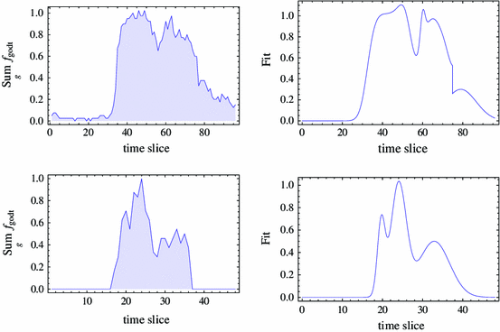

  

  Profiles used for generating the daily request $f_{godt}$: on the left side the original request, on the right side the interpolation used to generate the data.

• The number of weeks in the time horizon, $|\mathcal {O}|$, is uniformly extracted from $\{1,\ldots ,4\}$, while we always set $\mathcal {D}= \{1,\ldots ,7\}$ and $\mathcal {T}= \{ 1,\ldots ,48 \}$ (the time slices are half an hour long).

• The demand profile $f_{godt}$ is given by $p_g \cdot \mathcal {N}\cdot \text {Rand}(0.8,1.2) \cdot$ profile $(t)$, where $\mathcal {N}$ is a random integer variable uniformly extracted from $\{10,11,\ldots ,50\}$, Rand($x,y$) is a random real coefficient uniformly distributed between $x$ and $y$, profile($t$) is one of the two profiles mentioned earlier to reproduce a realistic evolution of the demand along each day of the week; finally, the $p_{g}$ coefficients are real random values uniformly extracted from $\left[ 0,1 \right]$ for each $g \in \mathcal {G}$ and normalized so that $\sum _{g \in \mathcal {G}} p_g = 1$.

• Parameter $\alpha$ is a random real value uniformly chosen in the range $[0.2, 0.6]$.

• The number of contracts $|\mathcal {M}|$ follows a uniform distribution in $\{3,\ldots ,10\}$. For synchronized contracts, $|\mathcal {S}_{1}|$ is uniformly distributed in $\{ 0,\ldots ,|\mathcal {M}| \}$, $|\mathcal {S}_{2}|$ in $\{ 0,\ldots ,|\mathcal {M}|-|\mathcal {S}_1| \}$ and $|\mathcal {S}_{3}|$ in $\{ 0,\ldots ,|\mathcal {M}|-|\mathcal {S}_1|-|\mathcal {S}_2| \}$. The number of contracts in $\mathcal {M}^{\mathrm {fix}}$ is zero if $|\cup _{m\in \mathcal {M}}\mathcal {W}_m| \le 1$, uniformly distributed in $\{ 0,1,2 \}$ otherwise.

• The number of weekly shift patterns $|\mathcal {W}_m|$ is uniformly distributed in $\{1,\ldots ,|\mathcal {O}|\}$ for each $m\in \mathcal {M}$.

• The limiting parameters $\Phi$, $v_{mt}$ and $V^{\max }_m$ are uniformly distributed in $\{\mathcal {N},\ldots ,\mathcal {N}+5\}$, $\{10,\ldots ,\mathcal {N}\}$ and $\{ \mathcal {N}/3,\mathcal {N}/2,\mathcal {N}\}$, respectively.

• The number of working shifts ranges from 2 to 6, and their length ranges from 4 to 9 h, i. e. from $\delta _h = 8$ to $\delta _h = 18$.

• The subset of shifts $\mathcal {H}_{mwd}$ is randomly extracted from $\mathcal {H}$ so as to guarantee that the rest shift ($h = 0$) and at least another work shift are available; we then set the number $N_{mwh}$ exploring the subsets $\mathcal {H}_{mwd}$ for all days $d \in \mathcal {D}$, so that we make sure that the required set of shifts over each week is feasible. We also make sure that there is at least one and no more than four resting days over the week so as to mimic realistic types of contracts.

• The subsets of time slices $\mathcal {T}_{mwdh} \subset \mathcal {T}$ are randomly generated with $|\mathcal {T}_{mwdh}|$ in $\{6,\ldots ,|\mathcal {T}|/3+6\}$. For synchronized contracts, we harmonize all of the $\mathcal {T}_{mwdh}$ for every $(d,h)$ pair so as to be sure that we can synchronize effectively.

• The maximum distance between 2 days of rest is $\Theta _m = |\mathcal {D}|$, that is one week, for all contracts.

• The shifts with $\delta _h < 14$ have no lunch breaks; the length of the lunch breaks is $\pi _{mh} = 1$ (half an hour) for 7 h shifts ($\delta _h = 14$), and $\pi _{mh}=2$ (1 h) for longer shifts. When a lunch break is expected, it must start at least $\eta _{mht} = 2$ time slices (1 h) after the beginning of the shift, and at least $\mu _{mht} = 4$ (2 h) before its end.

The structure of these instances is very complex and several parameters contribute to its definition. In particular, contrary to what usually occurs in standard optimization problems, it is not easy to identify one or two parameters which express the size of the instance. We have, therefore, generated a benchmark set of 50 instances as described above. Since our preliminary results indicated that we had generated instances with characteristics favoring the GRASP algorithm, we completed our set with 20 instances that differ from the first 50 through the new parameter ranges:

• $\mathcal {N}$ is uniformly extracted from $\{50,\ldots ,70\}$,

• $|\mathcal {G}|$ is uniformly extracted from $\{1,\ldots ,6\}$,

so as to avoid values of the variables $x_{gm}$ too close to 1.

We have analyzed a posteriori the computational time required, to classify the instances into groups of increasing size. This analysis shows that the product $P = |\mathcal {G}| \cdot |\mathcal {O}| \cdot |\mathcal {H}| \cdot \sum _{m \in \mathcal {M}} |\mathcal {W}_{m}|$ is highly correlated with the execution time. The log–log plot in Fig. 4 provides, on the left-hand side, the computational time required on each instance by the Rounding heuristic as a function of $P$. A linear fit of this plot gives a dependence of the running time on $P^{1.3}$, with a correlation coefficient $r^2 = 0.89$.

Fig. 4

Computational time in seconds required by the Rounding heuristic (left) and the GRASP heuristic (right) with respect to the size $P = |\mathcal {G}| \cdot |\mathcal {O}| \cdot |\mathcal {H}| \cdot \sum _{m \in \mathcal {M}} |\mathcal {W}_{m}|$ of each random instance, with logarithmic coordinates

Each single iteration of the GRASP heuristic also exhibits a dependence of the computational time on $P$, as reported in the log–log plot in the right-hand side of Fig. 4. In this case, the dependence is on $P^{0.7}$, which points to a better scalability of the GRASP algorithm. However, the correlation is much less pronounced, as the correlation coefficient is only $r^2=0.38$.

On the basis of the previous results, we have assumed the product $P$ as a meaningful measure of the size of the instances, and classified the $70$ generated instances into 7 classes of approximately 10 instances each. Table 4 contains the average results for these classes. Each class corresponds to a different row, and the last row reports the average results on the whole benchmark set: the first column shows the range of $P$ for the instances of the class, the second one the average computational time in seconds, the third and fourth columns the average percentage gap with respect to the best known solution. The last column provides the average number of GRASP iterations performed in the allotted time. As for the real instances, the computational time required by the Rounding heuristic has been measured and the same time has been assigned to the GRASP heuristic, to achieve a fair comparison.

Table 4 Computational results of the Rounding and the GRASP heuristics on the random instances

The average gap, in particular, on the larger instances, suggests that the GRASP heuristic has a slightly better performance. Such a conclusion, however, is not supported by statistical tests. Indeed, we have applied Wilcoxon’s matched-pairs signed-ranks test (Wilcoxon 1945) to the values of the objective function computed by the two algorithms on the 70 random instances. The test suggests that no clear dominance can be established between them.

However, a further analysis reveals an interesting dependence of the quality of the results on some features of the instances. More specifically, we observed that instances in which the $x_{gm}$ variables assume very small values tend to be solved more effectively by the GRASP algorithm than by the Rounding heuristic. This is not completely unexpected, as the rounding operations are necessarily more arbitrary and error-prone when performed on small values than when performed on large ones, whereas the GRASP heuristic works precisely optimizing the schedule of single operators with respect to the demand profile.

Of course, it is not very useful, though interesting, to identify a dependence of the results on features of the final solution (the average value of $x_{gm}$), which is unknown a priori. However, a similar correlation can be found considering, instead of $x_{gm}$ the ratio $\Gamma =\mathcal {N}/(|\mathcal {G}| \cdot |\mathcal {M}|)$ between the parameter which determines the peak of the demand profile in each instance and the product of the number of profiles and contract types. This index approximately describes the average number of operators required for each profile and contract to satisfy the demand. Figure 5 displays the gap between the best and the worst solution as a function of $\Gamma$ for each instance: the symbol indicates which algorithm produced the worst solution; algorithm Rounding is represented by circles while the GRASP is represented by triangles. This figure illustrates the effect of parameter $\Gamma$. For our generated instances, this parameter was fixed by us to generate consequently the demand; however, it can also be easily extracted from the raw data by computing the average value over the time horizon of the highest peak in the demand $\max _{t\in \mathcal {T}}\{\sum _{g{}} f_{godt}\}$.

Fig. 5

Distribution of the percent gap of the Rounding heuristic (circles) and the GRASP heuristic (triangles) with respect to the best known solution, as a function of the parameter $\mathcal {N}/(|\mathcal {G}| \cdot |\mathcal {M}|)$

As Fig. 5 suggests, when $\Gamma \in [0,1]$, the Rounding heuristic is at very clear disadvantage and there is no doubt that the GRASP heuristic is the way to go. A more ambiguous zone is the range $\Gamma \in [1,3]$ where the latter tends to show signs of weakness compared to the former. It is difficult to validate a clear dominance in this zone; however, one can note that when the GRASP heuristic proves worse, it tends to display a higher gap on average. Hence, it makes sense to favor the Rounding heuristic, to be statistically on the safe side. However, for values of $\Gamma > 3$, the Rounding heuristic takes over and dominates the competitor unambiguously. We can thus identify two ranges of the parameter where an algorithm is highly recommended over the other: for $\Gamma \in [0,1]$ the GRASP algorithm is better suited while for $\Gamma >3$ it is the Rounding algorithm that should be preferred. In between we recommend the comparison of the two heuristics, if the computational time available is enough.

The absence of a clear dominance between the two algorithms, together with the fact that rather frequently one of them has a clear advantage over the other, can be explained by this dependence on the features of the instance, which allows the user to choose which algorithm to use in each specific case, according to a measurable index.

Conclusions

We have proposed an extended model for simultaneous optimization of contract mix and personnel scheduling in call centers, further extending a previous model described in  Cordone et al. (2011). The resulting ILP model is considerably broader in its application, since it takes into account a large number of different contracts, even characterized by apparently “exotic” features. In this model, we can accommodate contracts with work-shifts of different duration, with limitations on their starting time or the days in which they can be used, possibly synchronized in different ways, as well as characterized by different possible shift patterns. Our model computes work-plans that comply with all legal constraints on the workload imposed to each operator. The model also includes lunch breaks scheduling.

The ILP model is very large and complex, with several mutually interacting constraints and integer variables. We designed two algorithms to solve it in a heuristic way. The Rounding algorithm is based on a decomposition of the model and it iterates the solution of the linear programming relaxation and an iterative rounding procedure. The GRASP algorithm is based on a greedy solution of a simplified single-operator model, and allows most problem instances to be solved in a few minutes and the largest instances in a few hours. Our computational experiments provide evidence that the two techniques are complementary to each other. We have also investigated indicators that can be computed to characterize a specific problem instance giving useful a priori indications on which algorithm is more likely to be more effective.

The two methods described in this paper have been implemented and used as a tool for analysis in real consulting situations in the telecommunication industry, in particular for call centers in a process of expansion and renovation, when trying to determine the best contracts that need to be defined to improve the level of service experienced by the customers.

References

Aksin Z, Armony M, Mehrotra V (2007) The modern call-center: a multi-disciplinary perspective on operations management research. Prod Oper Manag 16:655–688
Avramidis AN, Chan W, L’Écuyer P (2009) Staffing multi-skill call-centers via search methods and a performance approximation. IIE Trans 41:483–497
Avramidis T, Gendreau M, L’Écuyer P, Pisacane O (2007) Simulation-based optimization of agent scheduling in multiskill call centers, CORS/JOPT 2007, Montreal, Canada
Chan W, Avramidis T, L’Écuyer P (2007) Single Period Staffing for Multi-skill Call Centers, CORS/JOPT 2007, Montreal, Canada
Channouf N, L’Écuyer P, Avramidis T (2007) Models for Arrival Process in a Call Center, CORS/JOPT 2007, Montreal, Canada
Cordone R, Piselli A, Ravizza P, Righini G (2011) Optimization of multi-skill call-centers contracts and work-shifts. Serv Sci 3:67–81
Feo TA, Resende MGC (1989) A probabilistic heuristic for a computationally difficult set covering problem Oper Res Lett 8:67–71
Gans N, Koole G, Mandelbaum A (2003) Telephone call centers: tutorial. Rev Res Prospects Manuf Serv Oper Manag 5:79–141
Green LV, Kolesar PJ, Whitt W (2007) Coping with time-varying demand when setting staffing requirements for a service system. Prod Oper Manag 16:13–39
Pisacane O, Avramidis AN, Chan W, Gendreau M, L’Écuyer P (2006) Scheduling for Multi-Skill Call Centers, CORS/JOPT 2006, Montreal, Canada
Pot ASA (2006) Scheduling in Multi-Skill Call Centers, CORS/JOPT 2006, Montreal, Canada
Wallace RB, Whitt W (2005) A staffing algorithm for call-centers with skill-based routing. Manuf Serv Oper Manag 7:276–294
Wilcoxon F (1945) Individual Comparisons by Ranking Methods. Biometrics 1:80–83
Acknowledgments
The authors acknowledge the support of ACSU—Associazione Cremasca Studi Universitari to the OptLab, the Operations Research Laboratory of the University of Milan, where most part of this work was carried out. They also acknowledge the joint support of Studio Zeta srl and Regione Lombardia through the programme ”Dote Ricerca Applicata”. Two anonymous referees provided useful suggestions and comments.
Author information
Authors and Affiliations
Corresponding author
Rights and permissions
About this article
Cite this article
Cordone, R., Hosteins, P., Righini, G. et al. Optimal selection of contracts and work shifts in multi-skill call centers. EURO J Comput Optim 2, 247–277 (2014). https://doi.org/10.1007/s13675-013-0019-7
Received:
Accepted:
Published:
Issue Date:
DOI: https://doi.org/10.1007/s13675-013-0019-7