Logarithmically sparse symmetric matrices

Abstract

A positive definite matrix is called logarithmically sparse if its matrix logarithm has many zero entries. Such matrices play a significant role in high-dimensional statistics and semidefinite optimization. In this paper, logarithmically sparse matrices are studied from the point of view of computational algebraic geometry: we present a formula for the dimension of the Zariski closure of a set of matrices with a given logarithmic sparsity pattern, give a degree bound for this variety and develop implicitization algorithms that allow to find its defining equations. We illustrate our approach with numerous examples.

1 Introduction

Logarithmically sparse symmetric matrices are positive definite matrices for which the matrix logarithm is sparse. Such matrices arise in high-dimensional statistics (Battey 2017), where structural assumptions about covariance matrices are necessary for giving consistent estimators, and sparsity assumptions are natural to make. Moreover, once the sparsity pattern is fixed, the corresponding set of logarithmically sparse matrices forms a Gibbs manifold (Pavlov et al. 2023). As we recall in Sect. 2, this is a manifold obtained by applying the matrix exponential to a linear system of symmetric matrices (LSSM), here defined by the sparsity pattern. Gibbs manifolds play an important role in convex optimization (Pavlov et al. 2023, Section 5).

From the point of view of practical computations, it might be challenging to tell exactly whether a given matrix satisfies a given logarithmic sparsity pattern. Checking whether a given polynomial equation holds on the matrix is often much easier. This motivates studying Zariski closures of families of logarithmically sparse matrices, i.e. common zero sets of polynomials that vanish on such families. Such Zariski closures are examples of Gibbs varieties.

In this paper we study Gibbs varieties that arise as Zariski closures of sets of logarithmically sparse symmetric matrices. We explain how those can be encoded by graphs, give a formula for their dimension, and show that in practice it can be computed using simple linear algebra. We present a numerical and a symbolic algorithm for finding their defining equations. We also investigate how graph colorings can affect the corresponding Gibbs variety. In addition, we prove some general results about Gibbs varieties. In particular, we give an upper bound for the degree of a Gibbs variety in the case when the eigenvalues of the corresponding LSSM are $\mathbb {Q}$-linearly independent and show that Gibbs varieties of permutation invariant LSSMs inherit a certain kind of symmetry.

Our study of logarithmic sparsity is primarily motivated by statistics. A typical problem in high-dimensional statistics is estimating the covariance matrix of a random vector of length n from $l \ll n$ samples. It is known that no consistent estimator can be derived in such setup without making additional assumptions on the structure of the covariance matrix. This problem can in some cases be solved by assuming that the covariance matrix has a fixed logarithmic sparsity pattern (Battey 2017, 2023). An advantage of this assumption is that once a logarithmic sparsity pattern is induced on the covariance matrix C, it is also automatically induced on the concentration matrix $K = C^{-1}$, since $(\exp {L})^{-1} = \exp {(-L)}$. In principle, one could relax the structural assumption of logarithmic sparsity and replace it by the assumption that the covariance matrix is an element of the Gibbs variety. The advantage of such relaxation is that checking whether a given set of polynomial equations is satisfied by the matrix is generally simpler than computing the matrix logarithm and then checking whether it satisfies the sparsity condition.

Logarithmic sparsity also arises in entropic regularization of semidefinite programming (Pavlov et al. 2023, Section 5). In this context, sets of matrices satisfying a fixed logarithmic sparsity pattern are Gibbs manifolds that correspond to a particular class of SDP constraints. Namely, if the sparsity pattern is given by a graph G as explained in Sect. 3, the spectrahedron consists of PSD matrices for which some of the entries are fixed.

This paper is organized as follows. In Sect. 2, we define Gibbs manifolds and Gibbs varieties, the geometric objects needed for our research, present a formula for the dimension and an upper bound for the degree of Gibbs varieties, study symmetries of their defining equations and suggest a numerical implicitization algorithm. In Sect. 3, we give a formal definition of logarithmic sparsity, explain how it can be encoded by graphs and discuss the special properties of Gibbs varieties defined by logarithmic sparsity. In Sect. 4, we study families of logarithmically sparse matrices that arise from trees. In Sect. 5, we study colored logarithmic sparsity conditions. We conclude in Sect. 6 with a symbolic implicitization algorithm for Gibbs varieties defined by logarithmic sparsity.

2 Gibbs manifolds and Gibbs varieties

Let $\mathbb {S}^n$ denote the space of $n\times n$ symmetric matrices. This is a real vector space of dimension $\left( {\begin{array}{c}n+1\\ 2\end{array}}\right)$. The cone of positive semidefinite $n\times n$ matrices will be denoted by $\mathbb {S}^n_+$.

The matrix exponential function is defined by the usual power series, which converges for all real and complex $n \times n$ matrices. It maps symmetric matrices to the set of positive definite symmetric matrices $\textrm{int} (\mathbb {S}^n_+)$. The zero matrix $0_n$ is mapped to the identity matrix $\textrm{id}_n$. We write

$$\begin{aligned} \textrm{exp} \,:\, \mathbb {S}^n \rightarrow \textrm{int} (\mathbb {S}^n_+), \,\, X \,\mapsto \, \sum _{i=0}^\infty \, \frac{1}{i !} \,X^i. \end{aligned}$$

This map is invertible, with the inverse being the matrix logarithm function, defined on the set of positive definite matrices by the series

$$\begin{aligned} \textrm{log}\,\,:\, \textrm{int} (\mathbb {S}^n_+) \rightarrow \mathbb {S}^n ,\,\, Y \,\mapsto \, \sum _{j=1}^\infty \frac{(-1)^{j-1}}{j} \,( \,Y - \textrm{id}_n)^j. \end{aligned}$$

We next introduce the geometric objects that will play a crucial role in this article. We fix d linearly independent matrices $A_1, A_2,\ldots ,A_d$ in $\mathbb {S}^n$. We write $\mathcal {L}$ for $\textrm{span}_{\mathbb {R}}(A_1, \ldots , A_d)\,$, a linear subspace of the vector space $\mathbb {S}^n \simeq \mathbb {R}^{\left( {\begin{array}{c}n+1\\ 2\end{array}}\right) }$. Thus, $\mathcal {L}$ is a linear space of symmetric matrices (LSSM). We are interested in the image of $\mathcal {L}$ under the exponential map:

Definition 2.1

The Gibbs manifold $\textrm{GM}(\mathcal {L})$ of $\mathcal {L}$ is the d-dimensional manifold $\textrm{exp}(\mathcal {L}) \subset \mathbb {S}^n_+$.

This is indeed a d-dimensional manifold inside the convex cone $\mathbb {S}^n_+$. It is diffeomorphic to $\mathcal {L} \simeq \mathbb {R}^d$, with the diffeomorphism given by the exponential map and the logarithm map.

In some special cases (e.g. Pavlov et al. 2023, Theorem 6.1), the Gibbs manifold is semialgebraic. However, this fails in general. It is still interesting to ask which polynomial relations hold between the entries of any matrix in $\textrm{GM}(\mathcal {L})$. This motivates the following definition.

Definition 2.2

The Gibbs variety $\textrm{GV}(\mathcal {L})$ of $\mathcal {L}$ is the Zariski closure of $\textrm{GM}(\mathcal {L})$ in $\mathbb {C}^{\left( {\begin{array}{c}n+1\\ 2\end{array}}\right) }$.

Any LSSM can be written in the form $\mathcal {L} = \{y_1A_1+\ldots +y_dA_d|y_i\in \mathbb {R}\}$ and therefore can be identified with a matrix with entries in the field $\mathbb {R}(y_1,\ldots ,y_d)$ of rational functions in variables $y_1,\ldots ,y_d$. The eigenvalues of this matrix are algebraic functions of $y_1,\ldots ,y_d$ (elements of the algebraic closure $\overline{\mathbb {R}(y_1,\ldots ,y_d)}$) and will be referred to as the eigenvalues of the corresponding LSSM $\mathcal {L}$.

Example 2.3

Consider the LSSM spanned by $A_1 = \begin{pmatrix} 1 &{}\quad 0\\ 0 &{}\quad 1 \end{pmatrix}$ and $A_2 = \begin{pmatrix} 0 &{}\quad 1\\ 1 &{}\quad 0\end{pmatrix}$. It is identified with the matrix $\begin{pmatrix} y_1 &{}\quad y_2\\ y_2 &{}\quad y_1 \end{pmatrix}$ over $\mathbb {R}(y_1,y_2)$. Its eigenvalues are $\lambda _1 = y_1-y_2$ and $\lambda _2 = y_1+y_2$.

It is known that $\textrm{GV}(\mathcal {L})$ is irreducible and unirational under the assumption that the eigenvalues of $\mathcal {L}$ are $\mathbb {Q}$-linearly independent and $\mathcal {L}$ is defined over $\mathbb {Q}$ (Pavlov et al. 2023, Theorem 3.6).

In this section we extend the results of Pavlov et al. (2023) that apply to any LSSM $\mathcal {L}$. We start with studying the symmetries of the equations in the radical ideal of $\textrm{GV}(\mathcal {L})$.

We consider the tuple of variables $\textbf{x} = \{x_{ij} | 1\leqslant i \leqslant j \leqslant n\}$. An element $\sigma$ of the symmetric group $S_n$ acts on the polynomial ring $\mathbb {R}[\textbf{x}]$ by sending $x_{ij}$ to $x_{\sigma (i) \sigma (j)}$ for $1\leqslant i \leqslant j \leqslant n$ (we identify the variables $x_{ij}$ and $x_{ji}$). We will also consider the action of $S_n$ on $\mathbb {S}^n$ by simultaneously permuting rows and columns of a matrix.

Proposition 2.4

Let $\mathcal {L}$ be an LSSM of $n \times n$ matrices that is invariant under the action of $\sigma \in S_n$ as a set, i.e. $\sigma (\mathcal {L}) = \mathcal {L}$. Then the ideal $I({\textrm{GV}}(\mathcal {L}))$ of the corresponding Gibbs variety is also invariant under the action of $\sigma$.

Proof

To prove the Proposition, it suffices to show that if $B \in \mathcal {L}$ is obtained from $A \in \mathcal {L}$ by simultaneously permuting rows and columns, then $\exp {(B)}$ is obtained from $\exp {(A)}$ in the same way. Since $\exp {(B)}$ is a formal power series in B, it suffices to show that $B^k$ is obtained from $A^k$ by simultaneously permuting rows and columns for any non-negative integer k. The latter fact immediately follows from the matrix multiplication formula. $\square$

Note that Proposition 2.4 is equivalent to the well-known fact that $\exp {(P^{-1}AP)} = P^{-1}\exp {(A)}P$ for a permutation (and, more generally, orthogonal) matrix P.

In Sect. 3, we use Proposition 2.4 to show that ideals of Gibbs varieties of sparse LSSMs defined by graphs are invariant under permutations of variables induced by graph automorphisms.

Example 2.5

Consider the LSSM

$$\begin{aligned}\mathcal {L} = \left\{ \begin{pmatrix} y_1+y_2+y_3 &{}\quad y_1 &{}\quad y_2\\ y_1 &{}\quad y_1+y_2+y_3 &{}\quad y_3\\ y_2 &{}\quad y_3 &{}\quad y_1 + y_2 + y_3 \end{pmatrix} \bigg | y_1, y_2, y_3 \in \mathbb {R} \right\} .\end{aligned}$$

This linear space is spanned by the matrices

$$\begin{aligned} A_1 = \begin{pmatrix} 1 &{}\quad 1 &{}\quad 0\\ 1 &{}\quad 1 &{}\quad 0\\ 0 &{}\quad 0 &{}\quad 1 \end{pmatrix},~ A_2 = \begin{pmatrix} 1 &{}\quad 0 &{}\quad 1\\ 0 &{}\quad 1 &{}\quad 0\\ 1 &{}\quad 0 &{}\quad 1 \end{pmatrix},~ A_3 = \begin{pmatrix} 1 &{}\quad 0 &{}\quad 0\\ 0 &{}\quad 1 &{}\quad 1\\ 0 &{}\quad 1 &{}\quad 1 \end{pmatrix}. \end{aligned}$$

The transposition $\sigma = (1 2) \in S_3$ acts on $\mathbb {S}^3$ in the following way:

$$\begin{aligned}\begin{pmatrix} x_{11} &{}\quad x_{12} &{}\quad x_{13}\\ x_{12} &{}\quad x_{22} &{}\quad x_{23}\\ x_{13} &{}\quad x_{23} &{}\quad x_{33} \end{pmatrix} \mapsto \begin{pmatrix} x_{22} &{}\quad x_{12} &{}\quad x_{23}\\ x_{12} &{}\quad x_{11} &{}\quad x_{13}\\ x_{23} &{}\quad x_{13} &{}\quad x_{33} \end{pmatrix}.\end{aligned}$$

This action restricts to a linear automorphism of $\mathcal {L}$ defined by sending $A_2$ to $A_3$ and $A_3$ to $A_2$, while leaving $A_1$ intact. The Gibbs variety of $\mathcal {L}$ is a hypersurface in $\mathbb {C}^6$ whose prime ideal is generated by a single polynomial

$$\begin{aligned} p(x_{11},x_{12},x_{13},x_{22},x_{23},x_{33})= & {} (x_{11}-x_{22})(x_{11}-x_{33})(x_{22}-x_{33}) \\ {}{} & {} - x_{33}(x_{13}^2-x_{23}^2) - x_{22}(x_{23}^2-x_{12}^2) - x_{11}(x_{12}^2 -x_{13}^2). \end{aligned}$$

The action of $\sigma$ on $\mathbb {C}[x_{11},x_{12},x_{13},x_{22},x_{23},x_{33}]$ sends p to $-p$ and therefore does not change the ideal.

Definition 2.6

Let A be an $n\times n$ matrix, and $\mathcal {L}$ be an LSSM of $n \times n$ matrices. The centralizer C(A) of A is the set of all matrices that commute with A. The $\mathcal {L}$-centralizer $C_\mathcal {L}(A)$ of A is $C(A) \cap \mathcal {L}$.

Note that $C_\mathcal {L}(A)$ is a linear subspace of $\mathcal {L}$. Its dimension is independent of A for a generic choice of $A\in \mathcal {L}$ (see Sect. 3 for an explanation). This generic dimension will be denoted by k in Theorem 2.9. Here and further on in this paper the word “generic” is used in the standard sense of algebraic geometry and means “avoiding a subvariety of positive codimension”.

Gibbs manifolds can be conveniently parametrized using Sylvester’s formula.

Theorem 2.7

(Sylvester 1883) Let $f: D \rightarrow \mathbb {R}$ be an analytic function on an open set $D \subset \mathbb {R}$ and $M \in \mathbb {R}^{n \times n}$ a matrix that has n distinct eigenvalues $\lambda _1,\ldots ,\lambda _n$ in D. Then

$$\begin{aligned} f(M) \,=\, \sum \limits _{i=1}^{n}f(\lambda _i)M_i, \quad \text {with} \quad M_i \,=\, \prod _{j\ne i}\dfrac{1}{\lambda _i-\lambda _j}(M - \lambda _j \cdot \textrm{id}_n).\end{aligned}$$

We note that the product on the right hand side is a polynomial in M and therefore does not depend on the order of factors.

We will also need a version of the Ax–Schanuel Theorem (Ax 1971, Statement (SP)).

Theorem 2.8

(Ax–Schanuel) If the eigenvalues $\lambda _1,\ldots ,\lambda _n$ of the LSSM $\,\mathcal {L}$ are $\mathbb {Q}$-linearly independent, then $e^{\lambda _1}, \ldots , e^{\lambda _n}$ are algebraically independent over the field $\,\mathbb {C}(y_1,\ldots ,y_d)$.

The following theorem gives a formula for the dimension of Gibbs varieties. It is an extension of Pavlov et al. (2023, Theorem 2.4) in which only an inequality for dimension was given.

Theorem 2.9

Let $\mathcal {L}$ be an LSSM of $n\times n$ matrices of dimension d. Assume that $\mathcal {L}$ has distinct eigenvalues. Let k be the dimension of the $\mathcal {L}$-centralizer of a generic element in $\mathcal {L}$ and m the dimension of the $\mathbb {Q}$-linear space spanned by the eigenvalues of $\mathcal {L}$. Then $\dim \textrm{GV}(\mathcal {L}) = m + d - k$.

Proof

The characteristic polynomial of $A(y) = y_1 A_1 + \cdots + y_d A_d \in \mathcal {L}$ equals

$$\begin{aligned} P_{\mathcal {L}}(\lambda ;y) \,=\, \, c_0(y) + c_1(y) \, \lambda + \cdots + c_{n-1}(y) \, \lambda ^{n-1} + (-1)^n \, \lambda ^n. \end{aligned}$$

Its zeros $\lambda$ are algebraic functions of the coordinates $y = (y_1, \ldots , y_d)$ on $\mathcal {L}$.

Sylvester’s formula writes the entries of $\textrm{exp}(A(y))$ as rational functions of $y, \lambda _i(y)$ and $e^{\lambda _i(y)}$ for $y \in U$. They evaluate to convergent power series on $\mathbb {R}^d$.

Let V be the subvariety of $U \times \mathbb {R}^n$ that is defined by the equations

$$\begin{aligned} c_i(y) \, = \, (-1)^i \sigma _{n-i}(\lambda ) \quad \textrm{for} \quad i = 0, \ldots , n-1, \end{aligned}$$

(1)

where $\sigma _t(\lambda )$ is the $t^\textrm{th}$ elementary symmetric polynomial evaluated at $(\lambda _1, \ldots , \lambda _n)$. We have $\dim V = d$. Let $V'$ be any irreducible component of V. All irreducible components of V are equivalent under a permutation of the variables $\lambda _i$, so $\dim V' = d$.

Suppose that the eigenvalues of $\mathcal {L}$ satisfy some non-trivial linear relation over $\mathbb {Q}$. We can then find nonnegative integers $\alpha _i$ and $\beta _j$, not all zero, such that

$$\begin{aligned} \sum _{i=1}^n \alpha _i \lambda _i = \sum _{j=1}^n \beta _j \lambda _j. \end{aligned}$$

(2)

This implies that the exponentials of the eigenvalues satisfy the toric relation

$$\begin{aligned} \prod _{i=1}^n z_i^{\alpha _i} \,\, = \,\, \prod _{j=1}^n z_j^{\beta _j}. \end{aligned}$$

(3)

Let $I_W$ be the toric ideal generated by all such toric relations for $\mathcal {L}$. Let W be the toric variety defined by $I_W$. Note that by Theorem 2.8, $I_W$ contains all polynomial relations that hold between the exponentials of the eigenvalues of $\mathcal {L}$ and we have $\dim W = m$.

Define a map $\phi : V' \times W \rightarrow \mathbb {S}^n$, using coordinates $z_1, \ldots , z_n$ on $\mathbb {R}^n$, as follows:

$$\begin{aligned} (y_1, \ldots , y_d, \lambda _1, \ldots , \lambda _n, z_1, \ldots , z_n) \, \longmapsto \, \sum _{i=1}^n z_i \, \prod _{j \ne i} \frac{1}{\lambda _i-\lambda _j} (A(y) - \lambda _j \cdot \textrm{id}_n).\nonumber \\ \end{aligned}$$

(4)

By Sylvester’s formula, the map $\phi$ parametrizes the Gibbs variety (see Pavlov et al. 2023, Algorithm 1).

A generic fiber of $\phi$ consists of matrices that have the same set of eigenvectors. Two symmetric matrices have common eigenvectors if and only if they commute. Thus, the dimension of a generic fiber of $\phi$ is equal to the dimension of the centralizer of a generic element in this fiber, i.e. to k. The domain of $\phi$ is irreducible, being the product of irreducible varieties, and has dimension $m+d$. The variety $\textrm{GV}(\mathcal {L})$ is also irreducible by Pavlov et al. (2023, Theorem 3.6). Thus, by fiber dimension theorem (Hartshorne 1977, Exercise II.3.22) $\dim \textrm{GV}(\mathcal {L}) = m+d-k$. $\square$

We now give a degree bound for the Gibbs variety of an LSSM $\mathcal {L}$. In what follows, $\mathbb {V}(I)$ denotes the variety (over $\mathbb {C}$) defined by the polynomial ideal I.

Proposition 2.10

Let $\mathcal {L}$ be an LSSM of $n\times n$ matrices with $\mathbb {Q}$-linearly independent eigenvalues. Then $\deg \textrm{GV} (\mathcal {L}) \leqslant n^{\left( {\begin{array}{c}n+1\\ 2\end{array}}\right) +2n}$.

Proof

By Pavlov et al. (2023, Algorithm 1) the prime ideal J of $\textrm{GV}(\mathcal {L})$ is obtained by elimination from the ideal $I \subseteq \mathbb {C}[x_{ij},\lambda _i,z_i,y_i]$ of a polynomial ring in $\left( {\begin{array}{c}n+1\\ 2\end{array}}\right) + 2n + d$ variables generated by polynomials of degree at most n. By Michałek and Sturmfels (2021, Theorem 4.2) the variety $\mathbb {V}(J)$ is a projection of $\mathbb {V}(I)$ and therefore $\deg \mathbb {V}(J) \leqslant \deg \mathbb {V}(I)$. Therefore, $\deg \textrm{GV}(\mathcal {L}) = \deg \mathbb {V}(J) \leqslant \deg \mathbb {V}(I)$. The variety $\mathbb {V}(I)$ lives in the affine space of dimension $\left( {\begin{array}{c}n+1\\ 2\end{array}}\right) + 2n + d$, where $d=\dim \mathcal {L}$. Note that $\dim \mathbb {V}(I) \geqslant \dim \mathcal {L}$ and thus ${\text {codim}} \mathbb {V}(I) \leqslant \left( {\begin{array}{c}n+1\\ 2\end{array}}\right) +2n$. Therefore, by Bézout’s theorem (Fulton 1998, Theorem 12.3) we have $\deg \mathbb {V}(I) \leqslant n^{\left( {\begin{array}{c}n+1\\ 2\end{array}}\right) +2n}$, which proves the proposition. $\square$

As we will see below, the bound from Proposition 2.10 is pessimistic.

Once the degree of the Gibbs variety is known, one can use numerical techniques to find its defining equations. In general, this allows to compute ideals of Gibbs varieties that are infeasible for symbolic algorithms.

We now present Algorithm 1 for finding the equations of the Gibbs variety numerically. This is based on the ideas of Breiding et al. (2018, Chapter 5). We write $\langle P \rangle$ for the ideal generated by $P\subseteq \mathbb {C}[\textbf{x}]$.

Algorithm 1

Numerical implicitization of Gibbs varieties of known degree

Correctness of Algorithm 1 is ensured by the genericity condition imposed on the samples picked in Step .

Unfortunately, the degree upper bound in Proposition 2.10 restricts the practical applicability of this algorithm to $n\leqslant 3$. However, if the Gibbs variety is a hypersurface, then the algorithm can terminate immediately after finding a single algebraic equation. The degree of this equation is usually much lower than the degree bound in Proposition 2.10 (for instance, the Gibbs variety in Example 2.5 is defined by a cubic, while the bound from Proposition 2.10 is equal to $3^{12}$) and therefore the defining equation can be found with this algorithm for larger n.

Remark 2.11

Although Algorithm 1 uses floating point computations, for LSSMs defined over $\mathbb {Q}$ it can be adapted to give exact equations. This can be done using built-in commands in computer algebra systems, e.g. rationalize in Julia. Correctness of the rationalization procedure can be checked by plugging a parametrization of the Gibbs variety into the resulting equations.

3 Logarithmic sparsity patterns

Every simple undirected graph G on n nodes with edge set $E(G) \subseteq \{(i,j)|1 \leqslant i < j \leqslant n\}$ defines a sparsity pattern on $n\times n$ symmetric matrices in the following way.

Definition 3.1

We say that $A = (a_{ij}) \in \mathbb {S}^n$ satisfies the sparsity condition given by G if $a_{ij}=0$ whenever $i\ne j$ and $(i,j)\not \in E(G)$. Note that the diagonal entries of a matrix are never constrained to be zero. The set of all symmetric matrices satisfying the sparsity condition given by G forms an LSSM, which we will denote by $\mathcal {L}_G$.

Note that if G has n nodes and e edges, then $\dim \mathcal {L}_G = n+e$.

Example 3.2

Let $n=4$ and $E(G) = \{(2,3),(1,4)\}$. The corresponding LSSM

$$\begin{aligned}\mathcal {L}_G = \begin{pmatrix} y_{11} &{}\quad 0 &{}\quad 0 &{}\quad y_{14}\\ 0 &{}\quad y_{22} &{}\quad y_{23} &{}\quad 0\\ 0 &{}\quad y_{23} &{}\quad y_{33} &{}\quad y_{34}\\ y_{14} &{}\quad 0 &{}\quad y_{34} &{}\quad y_{44} \end{pmatrix}\end{aligned}$$

is cut out by the equations $y_{12} = y_{13} = y_{24} = 0$.

Definition 3.3

We say that $A \in \textrm{int}{(\mathbb {S}_+^n)}$ satisfies the logarithmic sparsity condition given by G if $\log {A} \in \mathcal {L}_G$.

We are interested in an algebraic description of the set of matrices that satisfy a logarithmic sparsity pattern given by G. This set of matrices is precisely the Gibbs manifold of $\mathcal {L}_G$. Since disconnected graphs correspond to LSSMs with block-diagonal structure and block-diagonal matrices are exponentiated block-wise, we will only consider the case of connected G.

We note that an automorphism $\sigma$ of a graph G does not change the associated linear space but induces a permutation of variables $\textbf{x}$ (namely, $x_{ij}$ is sent to $x_{\sigma (i)\sigma (j)}$). Therefore, by Proposition 2.4, the ideal of the Gibbs variety of $\mathcal {L}_G$ in the polynomial ring $\mathbb {C}[\textbf{x}]$ is invariant under permutations of variables induced by automorphisms of G.

LSSMs given by graphs are nice in the sense that finding the dimension of their Gibbs varieties can be reduced to a simple linear algebra procedure of computing matrix centralizers. This is justified by the following result.

Proposition 3.4

Let $\mathcal {L}_G$ be an LSSM given by a simple connected graph G on n nodes. Then its eigenvalues are $\mathbb {Q}$-linearly independent.

Proof

By setting the variables $y_{ij}$ to zero for $i\ne j$ and the variables $y_{ii}$ to n $\mathbb {Q}$-linearly independent algebraic numbers, we obtain a diagonal element of $\mathcal {L}_G$ whose eigenvalues are linearly independent over $\mathbb {Q}$. This immediately implies $\mathbb {Q}$-linear independence of the eigenvalues of $\mathcal {L}_G$. $\square$

We now address the question of computing the $\mathcal {L}_G$-centralizer of a generic element $A \in \mathcal {L}_G$. One way to do this is by straightforwardly solving the system of $\left( {\begin{array}{c}n\\ 2\end{array}}\right)$ equations $XA-AX = 0$ in the variables $x_{ij}$ over the field $\mathbb {Q}(a_{ij})$ (the minimal field over which the coefficients of the system are defined), where $x_{ij}$ are the entries of $X \in \mathcal {L}_G$ and $a_{ij}$ are the entries of A. However, there is a way to give a more explicit description of the $\mathcal {L}_G$-centralizer.

Note that by Proposition 3.4 the eigenvalues of $\mathcal {L}_G$ are $\mathbb {Q}$-linearly independent. In particular, this implies that the eigenvalues of $A \in \mathcal {L}_G$ are generically distinct and that A is generically non-derogatory (Horn and Johnson 1985, Definition 1.4.4). Therefore, by Horn and Johnson (1991, Theorem 4.4.17, Corollary 4.4.18) we have $C(A) = \textrm{span}_\mathbb {R}(\textrm{id}_n,A,\ldots ,A^{n-1})$, where $\textrm{id}_n$ is the $n\times n$ identity matrix. Hence, finding $C_{\mathcal {L}_G}(A)$ reduces to intersecting $\textrm{span}_\mathbb {R}(\textrm{id}_n,A,\ldots ,A^{n-1})$ with $\mathcal {L}_G$. Such an intersection can be found by solving a system of linear equations $p_0\textrm{id}_n + p_1A + \ldots + p_{n-1}A^{n-1} = \sum \limits _{(i,j)\not \in E_G} c_{ij}E_{ij}$ in the variables $p_0,\ldots ,p_{n-1},c_{ij}$. Since $\textrm{id}_n$ and A are both in $\mathcal {L}_G$, the intersection is at least two-dimensional and we arrive at the following proposition.

Proposition 3.5

Let G be a simple connected graph on n nodes with e edges. Then $\dim \textrm{GV} (\mathcal {L}_G) \leqslant 2n+e-2$.

Note that by the same argument, the upper bound $n+d-1$ from Pavlov et al. (2023, Theorem 2.4) for the dimension of the Gibbs variety of an arbitrary LSSM can be improved to $n+d-2$ for any LSSM containing the identity matrix.

Conjecture 3.6

We have $\dim \textrm{GV} (\mathcal {L}_G) = \min {\left( 2n+e-2,\left( {\begin{array}{c}n+1\\ 2\end{array}}\right) \right) }$.

When $2n+e-2 \leqslant \left( {\begin{array}{c}n+1\\ 2\end{array}}\right)$, Conjecture 3.6 is equivalent to the statement that $\{A^2,\ldots ,A^{n-1}\}\cup \{E_{ij} | (i,j) \in E(G)\} \cup \{E_{ii}|i=1,\ldots ,n\}$ is a linearly independent set. Here E(G) denotes the set of edges of G. This conjecture is true when G is a tree, as seen in the next section.

We end this section by characterizing Gibbs varieties for LSSMs that correspond to simple connected graphs on $n \leqslant 4$ vertices. Direct computation shows that for $n\leqslant 3$ we always have $\dim \textrm{GV}(\mathcal {L}_G) = \left( {\begin{array}{c}n+1\\ 2\end{array}}\right)$ and therefore $\textrm{GV}(\mathcal {L}_G)$ is the entire ambient space $\mathbb {C}^{\left( {\begin{array}{c}n+1\\ 2\end{array}}\right) }$. For $n=4$ there are 6 non-isomorphic simple connected graphs, 2 of which are trees. If G is not a tree, we once again have $\dim \textrm{GV}(\mathcal {L}_G) = 10 = \left( {\begin{array}{c}n+1\\ 2\end{array}}\right)$ and $\textrm{GV}(\mathcal {L}_G) = \mathbb {C}^{\left( {\begin{array}{c}n+1\\ 2\end{array}}\right) }$. If G is a tree, then $\textrm{GV}(\mathcal {L}_G)$ is a hypersurface. We discuss the defining equations of these 2 hypersurfaces in the next section.

4 Sparsity patterns given by trees

Trees are an important class of graphs that give rise to LSSMs with the smallest possible dimension for a given number of nodes. It is remarkable that for such LSSMs the dimension of the Gibbs variety only depends on the number of nodes in the graph (or, equivalently, the size of the matrices), and the dependence is linear. In what follows, we write $\mathbb {Q}(A)$ for the field of rational functions in the entries $a_{ij}$ of the matrix A over $\mathbb {Q}$.

Theorem 4.1

Let $\mathcal {L}_G$ be an LSSM given by a tree G on n nodes. Then ${\dim \textrm{GV}(\mathcal {L}_G) =3n-3}$.

Proof

By Proposition 3.4 the dimension of the $\mathbb {Q}$-linear space spanned by the eigenvalues of $\mathcal {L}_G$ is equal to n. The dimension of $\mathcal {L}_G$ is equal to $2n-1$, since G is a tree and therefore has $n-1$ edges. It remains to compute the dimension of the $\mathcal {L}_G$-centralizer of a generic element in $\mathcal {L}_G$. Suppose $A \in \mathcal {L}_G$. We are looking for solutions of the equation $AY-YA = 0$, $Y \in \mathcal {L}_G$. This is a system of homogeneous linear equations in the unknowns $y_{ij}$. We have $(AY-YA)_{ik} = \sum a_{ij}y_{jk} - \sum y_{ij}a_{jk}$. Note that since $Y \in \mathcal {L}_G$, $y_{ij}$ is generically non-zero if and only if (i, j) is an edge of G or $i=j$. The same is generically true for $a_{ij}$. Thus, $(AY-YA)_{ik}$ is not identically zero if and only if there exists j such that (i, j) and (j, k) are edges of G or if (i, k) is itself an edge of G. In terms of the graph G, this means that $(AY-YA)_{ik}$ is not identically zero if and only if there is a path of edge length at most 2 from i to k. Since G is a tree, there is at most one such path. Therefore, if i and k are connected by a path of edge length 2 via the node j, the corresponding entry of $AY-YA$ is equal to $a_{ij} y_{jk} - a_{jk}y_{ij}$. It is equal to zero if $y_{jk}$ is proportional to $y_{ij}$ with the coefficient $a_{ij}/a_{jk}$ (note that $a_{jk}$ is generically non-zero). Since G is connected, we conclude that all the $y_{ij}$ with $i\ne j$ are proportional to each other with coefficients prescribed by A. If i and k are connected by an edge, the corresponding entry of $AY-YA$ is equal to $y_{ii}a_{ik} - y_{kk}a_{ik} - (a_{ii}-a_{kk})y_{ik}$. If it is equal to zero, then $y_{kk} = y_{ii} - \dfrac{a_{ii}-a_{kk}}{a_{ik}} y_{ik}$. We conclude that, since G is connected and all the $y_{ik}$ are proportional to each other over $\mathbb {Q}(A)$, all the $y_{ii}$ can be expressed as $\mathbb {Q}(A)$-linear combinations of $y_{11}$ and just one $y_{jk}$ with $j\ne k$. Therefore, the centralizer, which is the solution space of the considered linear system, is at most 2-dimensional. Since it contains $\textrm{id}_n$ and A, it is exactly two-dimensional. The statement of the theorem now follows from Theorem 2.9 for $m = n$, $d=2n-1$ and $k=2$. $\square$

Example 4.2

For $n=4$ there are exactly two non-isomorphic trees, shown below. By Theorem 4.1, the dimension of their Gibbs varieties is equal to 9. Therefore, these Gibbs varieties are hypersurfaces in $\mathbb {C}^{\left( {\begin{array}{c}n+1\\ 2\end{array}}\right) }=\mathbb {C}^{10}$.

The corresponding LSSMs are

$$\begin{aligned} \begin{pmatrix} y_{11} &{}\quad y_{12} &{}\quad 0 &{}\quad 0\\ y_{12} &{}\quad y_{22} &{}\quad y_{23} &{}\quad 0 \\ 0 &{}\quad y_{23} &{}\quad y_{33} &{}\quad y_{34} \\ 0 &{}\quad 0 &{}\quad y_{34} &{}\quad y_{44} \end{pmatrix}\quad \text {and}\quad \begin{pmatrix} y_{11} &{}\quad y_{12} &{}\quad y_{13} &{}\quad y_{14}\\ y_{12} &{}\quad y_{22} &{}\quad 0 &{}\quad 0\\ y_{13} &{}\quad 0 &{}\quad y_{33} &{}\quad 0\\ y_{14} &{}\quad 0 &{}\quad 0 &{}\quad y_{44} \end{pmatrix}, \end{aligned}$$

respectively.

For the 4-chain, the graph on the left, the Gibbs variety is defined by a single homogeneous polynomial of degree 6 that has 94 terms:

$$\begin{aligned}x_{11}x_{12}x_{14}x_{23}^2 x_{34} - x_{11}x_{12}x_{14}x_{23}x_{24}x_{33} + \cdots - x_{14}^2 x_{22} x_{23} x_{34}^2 + x_{14}^2 x_{22} x_{24} x_{33} x_{34}.\end{aligned}$$

For the graph on the right the defining polynomial is also homogeneous of degree 6. It has 60 terms:

$$\begin{aligned}x_{11}x_{12}x_{13} x_{22} x_{24} x_{34} - x_{11} x_{12} x_{13} x_{23} x_{24}^2+\cdots - x_{14}^2 x_{23}^2 x_{34}^2 + x_{14}^2 x_{23} x_{24} x_{33} x_{34}.\end{aligned}$$

These two equations were found using Algorithm 1.

5 Logarithmic sparsity from colored graphs

Sparse LSSMs defined by colored graphs appear in the study of colored Gaussian graphical models in algebraic statistics (Højsgaard and Lauritzen 2008; Sturmfels and Uhler 2010). In this section, we study the properties of Gibbs varieties of such LSSMs.

Consider the graph G and suppose its vertices are labeled by p colors and edges are labeled by q colors. The corresponding LSSM $\mathcal {L}$ is cut out by the following three sets of equations.

• 1. $x_{ij} = 0$ if (i, j) is not an edge of G

• 2. $x_{ii} = x_{jj}$ if the vertices i and j have the same color.

• 3. $x_{ij} = x_{kl}$ if (i, j) and (k, l) are edges of G that have the same color.

It is immediately clear that $\dim \mathcal {L} = p+q$.

We will denote colored graphs by $\mathcal {G}$ and the corresponding LSSMs by $\mathcal {L}_\mathcal {G}$. The corresponding uncolored graph will be denoted by G, as usual. Note that since $\mathcal {L}_{\mathcal {G}} \subseteq \mathcal {L}_{G}$, the inclusion of the Gibbs varieties also holds: $\textrm{GV}(\mathcal {L}_\mathcal {G}) \subseteq \textrm{GV}(\mathcal {L}_G)$. Since the identity matrix is in $\mathcal {L}_\mathcal {G}$ for any $\mathcal {G}$, the dimension bound from Proposition 3.5 holds for colored graphs as well. This is reformulated in terms of numbers of colors in the following result.

Proposition 5.1

Let $\mathcal {G}$ be a colored graph on n nodes in which vertices are labeled by p colors and edges are labeled by q colors. Then $\dim \textrm{GV} (\mathcal {L}_\mathcal {G}) \leqslant n+p+q-2$.

Definition 5.2

We say that $X\in \mathbb {S}_+^n$ satisfies the colored sparsity pattern given by $\mathcal {G}$ if $X \in \mathcal {L}_\mathcal {G}$.

Note that if $\mathcal {G}$ is a colored graph, the eigenvalues of $\mathcal {L}_\mathcal {G}$ are not necessarily $\mathbb {Q}$-linearly independent. Therefore, the upper bound from Proposition 5.1 is not always attained.

Example 5.3

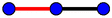
Consider the graph .

The corresponding LSSM is

$$\begin{aligned} \begin{pmatrix} y_1 &{}\quad y_2 &{}\quad 0\\ y_2 &{}\quad y_1 &{}\quad y_3\\ 0 &{}\quad y_3 &{}\quad y_1 \end{pmatrix}. \end{aligned}$$

The eigenvalues of this LSSM are $\mathbb {Q}$-linearly dependent: they satisfy the equation $2\lambda _2 = \lambda _1 + \lambda _3$. We have $\dim \textrm{GV}(\mathcal {L}) = 3 < n+p+q-2 = 3 + 1 + 2 - 2 =4$, which can be verified using Pavlov et al. (2023, Algorithm 1). Note that in this case $\dim \textrm{GV}(\mathcal {L}_\mathcal {G}) = \dim \textrm{GM}(\mathcal {L}_\mathcal {G})$.

In order to illustrate how different colorings of the same graph affect the Gibbs variety, we conclude this section with analysing colored graphs for which the underlying graph is the 3-chain. This is done using Pavlov et al. (2023, Algorithm 1).

• 1. The corresponding LSSM is

  $$\begin{aligned}\mathcal {L}_\mathcal {G} = \begin{pmatrix} y_1 &{}\quad y_4 &{}\quad 0\\ y_4 &{}\quad y_2 &{}\quad y_5\\ 0 &{}\quad y_5 &{}\quad y_3 \end{pmatrix}. \end{aligned}$$

  $\dim \textrm{GV}(\mathcal {L}_\mathcal {G}) = 6$ and there are no polynomial equations that hold on the Gibbs variety.

• 2. The corresponding LSSM is

  $$\begin{aligned}\mathcal {L}_\mathcal {G} = \begin{pmatrix} y_1 &{}\quad y_4 &{}\quad 0\\ y_4 &{}\quad y_2 &{}\quad y_4\\ 0 &{}\quad y_4 &{}\quad y_3 \end{pmatrix}.\end{aligned}$$

  $\dim \textrm{GV}(\mathcal {L}_\mathcal {G}) = 5$ and the Gibbs variety is a cubic hypersurface whose prime ideal is generated by the polynomial

  $$\begin{aligned}{} & {} x_{11}x_{13}x_{23}-x_{12}^2 x_{23} + x_{12}x_{22}x_{13}-x_{12}x_{13}^2\\{} & {} \quad -x_{12}x_{13}x_{33}+x_{12}x_{23}^2-x_{22}x_{13}x_{23}+x_{13}^2 x_{23}. \end{aligned}$$

• 3. The corresponding LSSM is

  $$\begin{aligned}\mathcal {L}_\mathcal {G} = \begin{pmatrix} y_1 &{}\quad y_3 &{}\quad 0\\ y_3 &{}\quad y_1 &{}\quad y_4\\ 0 &{}\quad y_4 &{}\quad y_2 \end{pmatrix}.\end{aligned}$$

  $\dim \textrm{GV}(\mathcal {L}_\mathcal {G}) = 5$ and the Gibbs variety is a cubic hypersurface. Its prime ideal is generated by the polynomial

  $$\begin{aligned}{} & {} -x_{11}x_{12}x_{23}+x_{11}x_{22}x_{13} - x_{11}x_{13}x_{33}+x_{12}x_{22}x_{23}\\{} & {} \quad -x_{22}^2 x_{13}+x_{22}x_{13}x_{33}+x_{13}^3-x_{13}x_{23}^2. \end{aligned}$$

• 4. The corresponding LSSM is

  $$\begin{aligned}\mathcal {L}_\mathcal {G} = \begin{pmatrix} y_1 &{}\quad y_3 &{}\quad 0\\ y_3 &{}\quad y_1 &{}\quad y_3\\ 0 &{}\quad y_3 &{}\quad y_2\\ \end{pmatrix}.\end{aligned}$$

  $\dim \textrm{GV}(\mathcal {L}_\mathcal {G}) = 4$. The Gibbs variety is a complete intersection, its prime ideal is generated by the polynomials

  $$\begin{aligned} x_{11} - x_{22} + x_{33}, \end{aligned}$$
  $$\begin{aligned} -x_{12}x_{23}+x_{22}x_{13}-x_{13}^2-x_{13}x_{33}+x_{23}^2. \end{aligned}$$

• 5. The corresponding LSSM is

  $$\begin{aligned}\mathcal {L}_\mathcal {G} = \begin{pmatrix} y_1 &{}\quad y_3 &{}\quad 0\\ y_3 &{}\quad y_2 &{}\quad y_4\\ 0 &{}\quad y_4 &{}\quad y_1 \end{pmatrix}. \end{aligned}$$

  $\dim \textrm{GV}(\mathcal {L}_\mathcal {G}) = 5$ and the Gibbs variety is a cubic hypersurface. Its prime ideal is generated by the polynomial

  $$\begin{aligned}-x_{11}x_{12}x_{23}+x_{12}^2 x_{13}+x_{12} x_{23} x_{33} - x_{13}x_{23}^2.\end{aligned}$$

  Rewriting this as $x_{12}(x_{12}x_{13}-x_{11}x_{23})+x_{23}(x_{12}x_{33}-x_{13}x_{23})$, we see that $\textrm{GV}(\mathcal {L}_{\mathcal {G}})$ contains the linear space $x_{12}=x_{23}=0$ and the toric variety $x_{12}x_{13}-x_{11}x_{23}=x_{12}x_{33}-x_{13}x_{23}=0$ as subvarieties of codimension one. Note that this Gibbs variety is stable under the linear automorphism of $\mathbb {S}^3$ given by exchanging $x_{12}$ and $x_{23}$. The same is true for the space $\mathcal {L}_G$ itself. This underscores that understanding which symmetries of the linear space $\mathcal {L}$ are inherited by its Gibbs variety beyond the context of Proposition 2.4 is an interesting question for future research.

• 6. The corresponding LSSM is

  $$\begin{aligned}\mathcal {L}_\mathcal {G} = \begin{pmatrix} y_1 &{}\quad y_3 &{}\quad 0\\ y_3 &{}\quad y_2 &{}\quad y_3\\ 0 &{}\quad y_3 &{}\quad y_1 \end{pmatrix}.\end{aligned}$$

  $\dim \textrm{GV}(\mathcal {L}_\mathcal {G}) = 4$ and the Gibbs variety is an affine subspace with the prime ideal generated by $x_{12}-x_{23}$ and $x_{11}-x_{33}$.

• 7. The corresponding LSSM

  $$\begin{aligned}\mathcal {L}_\mathcal {G} = \begin{pmatrix} y_1 &{}\quad y_2 &{}\quad 0\\ y_2 &{}\quad y_1 &{}\quad y_3\\ 0 &{}\quad y_3 &{}\quad y_1 \end{pmatrix}\end{aligned}$$

  appeared in Example 5.3. We have $\dim \textrm{GV}(\mathcal {L}_\mathcal {G}) = 3$. The prime ideal of the Gibbs variety is generated by seven polynomials:

  $$\begin{aligned}{} & {} x_{12}x_{13}-x_{22}x_{23}+x_{23}x_{33},\\{} & {} x_{11}x_{13}-x_{12}x_{23}+x_{13}x_{33},\\{} & {} x_{11}x_{22}-x_{11}x_{33}-x_{22}^2+x_{22}x_{33}+x_{13}^2,\\{} & {} x_{12}^2 - x_{22}^2 + x_{13}^2 + x_{33}^2,\\{} & {} x_{11}x_{12}-x_{12}x_{22}+x_{13}x_{23},\\{} & {} x_{11}^2-x_{22}^2+x_{13}^2+x_{23}^2,\\{} & {} -x_{12}x_{22}x_{23}+x_{12}x_{23}x_{33}+x_{22}^2 x_{13}-x_{13}^3-x_{13}x_{33}^2.\end{aligned}$$

• 8. The corresponding LSSM is

  $$\begin{aligned}\mathcal {L}_\mathcal {G} = \begin{pmatrix} y_1 &{}\quad y_2 &{}\quad 0\\ y_2 &{}\quad y_1 &{}\quad y_2\\ 0 &{}\quad y_2 &{}\quad y_1 \end{pmatrix}.\end{aligned}$$

  This is a commuting family and therefore, by Pavlov et al. (2023, Theorem 2.7) $\dim \textrm{GV}(\mathcal {L}_\mathcal {G}) = 2$ and $\textrm{GM}(\mathcal {L}_\mathcal {G}) = \textrm{GV}(\mathcal {L}_\mathcal {G}) \cap \textrm{int}(\mathbb {S}_+^3)$. The prime ideal of the Gibbs variety is generated by three linear forms and one quadric: $x_{22}-x_{13}-x_{33}$, $x_{12}-x_{23}$, $x_{11}-x_{33}$ and $-2x_{13}x_{33}+x_{23}^2$.

6 From analytic to algebraic equations

Since the logarithm is an analytic function on $\mathbb {R}_{>0}$, the set of matrices satisfying the logarithmic sparsity pattern given by a graph G can be defined via formal power series equations. One way to write these equations in a compact form is by using Sylvester’s formula (Theorem 2.7).

By setting f in Sylvester’s formula to be the logarithm function, we obtain a parametrization of $\log X$ with rational functions in the entries $x_{ij}$ of X, the eigenvalues $\lambda _i$ of X and their logarithms $\log \lambda _i$. The logarithmic sparsity condition induced on X requires that some components of this parametrization are zero and therefore gives a system of polynomial equations in $x_{ij}$, $\lambda _i$ and $\log {\lambda _i}$. By eliminating the variables $\lambda _i$ and $\log \lambda _i$ from this system while taking into account the polynomial relations between $\lambda _i$ and $x_{ij}$ given by the coefficients of the characteristic polynomial, we obtain a set of defining equations of $\textrm{GV}(\mathcal {L}_G)$. This procedure is described by Algorithm 2. The notation $I:a^\infty$ stands for saturation of an ideal I of a ring R by an element $a\in R$, that is, $I :a^{\infty }:= \{b \in R \mid \exists N \in \mathbb {Z}_{\geqslant 0} :a^Nb \in I\}$. The quantities $x_{ij}$, $\lambda _i$ and $\log \lambda _i$ are treated by the algorithm as variables in a polynomial ring, without a priori algebraic dependencies between them.

Algorithm 2

Implicitization of the Gibbs variety of $\mathcal {L}_G$ given by a graph G

Theorem 6.1

Algorithm 2 is correct. The ideal J computed in step  is the prime ideal of $\textrm{GV}(\mathcal {L}_G)$.

Proof

Since the eigenvalues of $\mathcal {L}_G$ are $\mathbb {Q}$-linearly independent, the ideal generated by $E_2$ is prime. Moreover, there is no $\mathbb {C}$-algebraic relation between the eigenvalues of X and their logarithms that holds for any positive definite X. This is a consequence of Theorem 2.8: any $\mathbb {Q}$-linear relation imposed on the logarithms of eigenvalues defines a set of positive codimension in the set of positive definite matrices, so one can assume that the logarithms of eigenvalues, considered as functions in the entries of an indeterminate positive definite matrix X, are $\mathbb {Q}$-linear independent and apply Theorem 2.8. These two facts ensure that all the algebraic relations between X, $\lambda$ and $\log \lambda$ are accounted for, and that the algorithm is thus correct. The ideal generated by $E_1$ and $E_2$ is therefore also prime, after saturation, and elimination in step  preserves primality. $\square$

Note that the primality of J means that $\textrm{GV}(\mathcal {L}_G)$ is irreducible, as stated in Pavlov et al. (2023, Theorem 3.6). The advantage of this algorithm compared to Pavlov et al. (2023, Algorithm 1) is that it uses a smaller polynomial ring and fewer variables are eliminated.

References

Ax, J.: On Schanuel’s conjectures. Ann. Math. 93(2), 252–268 (1971)
Battey, H.S.: Eigen structure of a new class of structured covariance and inverse covariance matrices. Bernoulli 23, 3166–3177 (2017)
Battey, H.S.: Inducement of population sparsity. Can. J. Stat. 51(3), 760–768 (2023)
Breiding, P., Kalisnik, S., Sturmfels, B., Weinstein, M.: Learning algebraic varieties from samples. Rev. Mat. Complut. 31, 545–593 (2018)
Fulton, W.: Intersection Theory. Springer, New York (1998)
Hartshorne, R.: Algebraic Geometry. Graduate Texts in Mathematics. Springer, New York (1977)
Højsgaard, S., Lauritzen, S.: Graphical Gaussian models with edge and vertex symmetries. J. R. Stat. Soc. 70, 1005–1027 (2008)
Horn, R.A., Johnson, C.R.: Matrix Analysis. Cambridge University Press, Cambridge (1985). https://doi.org/10.1017/CBO9780511810817
Horn, R.A., Johnson, C.R.: Topics in Matrix Analysis. Cambridge University Press, New York (1991). https://doi.org/10.1017/CBO9780511840371
Michałek, M., Sturmfels, B.: Invitation to Nonlinear Algebra. Graduate Studies in Mathematics, vol. 211. American Mathematical Society, Providence (2021)
Pavlov, D., Sturmfels, B., Telen, S.: Gibbs manifolds. Inf. Geom. (2023). https://doi.org/10.1007/s41884-023-00111-2
Sturmfels, B., Uhler, C.: Multivariate Gaussians, semidefinite matrix completion, and convex algebraic geometry. Ann. Inst. Stat. Math. 62, 603–638 (2010)
Sylvester, J.J.: On the equation to the secular inequalities in the planetary theory. Philos. Mag. Ser. 16, 267–269 (1883)
Acknowledgements
The author would like to thank Bernd Sturmfels, Simon Telen, and Piotr Zwernik for helpful discussions and suggestions. The author is grateful to anonymous referees for their helpful comments.
Funding
Open Access funding enabled and organized by Projekt DEAL.
Author information
Authors and Affiliations
Corresponding author
Ethics declarations
Conflict of interest
The author declares that there is no conflict of interest.
Additional information
Publisher's Note
Springer Nature remains neutral with regard to jurisdictional claims in published maps and institutional affiliations.
Rights and permissions
Open Access This article is licensed under a Creative Commons Attribution 4.0 International License, which permits use, sharing, adaptation, distribution and reproduction in any medium or format, as long as you give appropriate credit to the original author(s) and the source, provide a link to the Creative Commons licence, and indicate if changes were made. The images or other third party material in this article are included in the article’s Creative Commons licence, unless indicated otherwise in a credit line to the material. If material is not included in the article’s Creative Commons licence and your intended use is not permitted by statutory regulation or exceeds the permitted use, you will need to obtain permission directly from the copyright holder. To view a copy of this licence, visit http://creativecommons.org/licenses/by/4.0/.
About this article
Cite this article
Pavlov, D. Logarithmically sparse symmetric matrices. Beitr Algebra Geom (2024). https://doi.org/10.1007/s13366-024-00753-y
Received:
Accepted:
Published:
DOI: https://doi.org/10.1007/s13366-024-00753-y