Sobolev orthogonal polynomials, Gauss–Borel factorization and perturbations

Abstract

We present a comprehensive class of Sobolev bi-orthogonal polynomial sequences, which emerge from a moment matrix with an LU factorization. These sequences are associated with a measure matrix defining the Sobolev bilinear form. Additionally, we develop a theory of deformations for Sobolev bilinear forms, focusing on polynomial deformations of the measure matrix. Notably, we introduce the concepts of Christoffel–Sobolev and Geronimus–Sobolev transformations. The connection formulas between these newly introduced polynomial sequences and existing ones are explicitly determined.

1 Introduction

1.1 Historical background and motivation

Over the past few decades, the exploration of Sobolev orthogonal polynomials has evolved into a burgeoning field capturing increasing attention within the realms of Applied Mathematics and Mathematical Physics. This article aims to advance the concept of Sobolev orthogonality by presenting a comprehensive theoretical framework that facilitates the definition of an expansive set of Sobolev bi-orthogonal polynomial sequences (SBPS).

To situate our contribution within the existing scholarly landscape, we commence by highlighting key findings from the current body of literature. Our focus is specifically directed towards aspects of notable significance for our research. For a more comprehensive overview of contemporary results, historical context, and an up-to-date bibliography, interested readers are invited to consult [27] and [28].

The inception of Sobolev orthogonal polynomials dates back to 1962 with Althammer’s seminal work [2]. Althammer proposed a novel concept—namely, the definition of a polynomial class orthogonal in relation to a deformation of the Legendre inner product, as expressed by the following form:

$$\begin{aligned} \langle f,g \rangle _{A}= \int _{-1}^{1} f(x)g(x)\textrm{d}x + \lambda \int _{-1}^{1} f'(x) g'(x) \textrm{d}x. \end{aligned}$$

The polynomials stemming from this inner product are now commonly referred to as the Sobolev–Legendre polynomials.

Significant advancements in the theory emerged during the 1970s, particularly through notable contributions found in the works of [32] and [33]. In these influential studies, Schäfke and Wolf introduced a noteworthy family of inner products, laying a substantial foundation for the subsequent development of the field.

$$\begin{aligned} \langle f,g \rangle _{SW}= \sum _{j,k=0}^{\infty }\int _{a}^{b} f^{(j)}(x)g^{(k)}(x) v_{j,k}(x)w(x)\textrm{d}x. \end{aligned}$$

Here, the weight w and the corresponding integration interval are specifically intended to align with one of the three classical cases: Hermite, Laguerre, or Jacobi. Additionally, the functions $v_{j,k}(x)$ represent appropriate polynomials that exhibit symmetry in both indices, namely j and k.

Commencing with this polynomial deformation of classical measures and judiciously specifying the functions $v_{j,k}$, Schäfke and Wolf successfully defined eight new families of Sobolev orthogonal polynomials. Their work not only introduced these novel polynomial sequences but also extended the scope of all previously established results on Sobolev orthogonal polynomials.

A notable resurgence of interest in the field of Sobolev orthogonality has been evident since the last decade of the XX century, sparked by the influential paper [18]. This work introduced the concept of "coherent pairs," a fundamental idea that has spurred numerous subsequent developments. Consider a pair of Borel measures on the real line with finite moments, denoted as $\{d\mu _{1}, d \mu _{2}\}$. For this pair, an associated inner product is defined as $\langle f,g \rangle _{(\mu _{1}, \mu _{2})}= \int _{a}^{b} f(x)g(x)\,d \mu _{1} + \lambda \int _{a}^{b} f'(x) g'(x) \,d\mu _{2}$, where $a,b\in \mathbb {R}$. Essentially, the coherence of the pair $\{\textrm{d}\mu _{1}, \textrm{d}\mu _{2}\}$ is established when the sequence of polynomials associated with $\textrm{d}\mu _{2}$ can be intricately linked to the first derivatives of the polynomials associated with $\textrm{d}\mu _{1}$.

In the groundbreaking work by [25], a classification of coherent pairs was provided, specifically when one of the two involved measures is a classical one (Hermite, Laguerre, Jacobi, or Bessel). Additionally, [29] demonstrated that for $\{\textrm{d}\mu _{1}, \textrm{d}\mu _{2}\}$ to form a coherent pair, at least one of the two measures must be classical. This result underscored the completeness of the classification presented in [25].

In the work [20], the authors explore Sobolev bilinear forms represented as

$$\begin{aligned} B_N(p, q) = \sum _{i=0}^N \sum _{j=0}^N \left\langle \sigma _{i, j}, p^{(i)} q^{(j)} \right\rangle , \end{aligned}$$

where N is a fixed non-negative integer. In this expression, each $\sigma _{i, j}$ is a moment functional (i.e., a real or complex-valued linear functional on the space of real polynomials), $p^{(k)}$ denotes the kth derivative of the polynomial p, and $\langle \sigma , p \rangle$ indicates the action of $\sigma$ on p.

The authors in [22] establish necessary and sufficient conditions on $\sigma _{i, j}$ to ensure the symmetry of $B_N$. In the case of symmetry, a diagonal representation for $B_N$ emerges, taking the form $B_N(p, q) = \sum _{k=0}^N \left\langle \tau _k, p^{(k)} q^{(k)} \right\rangle$, where $\tau _k$ represents moment functionals for $k \in \{0, 1, \ldots , N\}$. A combinatorial interpretation of the coefficients present in the diagonal representation is provided in [20].

Furthermore, over the past two decades, a wealth of results has been established, spanning various analytic and algebraic facets of the theory. Noteworthy contributions include investigations into the relationship with differential operators [12, 21], the asymptotic behavior, and the examination of zeros of Sobolev polynomials [23], among other significant developments.

1.2 Main results

This paper presents a substantial generalization of the Schäfke and Wolf construction [33] by introducing a broad category of Sobolev bilinear forms $(*,*)_{\varvec{\mu }}$ that need not be symmetric. These forms are defined through a matrix of measures denoted as $\varvec{\mu }$, a fundamental mathematical structure in our investigation. For each measure matrix $\varvec{\mu }$, or equivalently, the corresponding bilinear form, a natural association exists with a moment matrix G.

Our analysis is specifically directed towards the class of moment matrices that possess an LU-factorization. Within this class, we can systematically generate Sobolev bi-orthogonal polynomial sequences (SBPS). Notably, we establish that numerous algebraic techniques associated with the LU-factorization, proven highly effective in deducing algebraic properties of standard orthogonal polynomial sequences (OPS), seamlessly extend to our Sobolev framework.

An essential concept introduced in this paper is that of additive Uvarov perturbations applied to a measure matrix $\varvec{\mu }$ within the Sobolev framework. Specifically, we delve into the study of conditions under which the introduction of an additive matrix perturbation to $\varvec{\mu }$ leads to the generation of families of Sobolev bi-orthogonal polynomial sequences (SBPS). This approach proves to be instrumental in extending the conventional methodology employed for discrete Sobolev bilinear forms.

Our investigation unfolds by splitting Sobolev bilinear functions into two distinctive components: a continuous part, which involves the entries of $\varvec{\mu }$ with continuous support, and a discrete part, encompassing entries with discrete support (e.g., $\delta$ distributions). Some authors categorize these types as type-I for continuous support only, and type-II and III for those involving continuous support along with finite subsets. Effectively interpreting the discrete part as an additive discrete perturbation of its continuous counterpart, we derive a compelling characterization of SBPS associated with the original measure matrix. This characterization is articulated through quasi-determinantal formulas, wherein only the continuous part of the bilinear function is involved.

Given the pivotal role of measure matrices in our approach, a natural concern arises: how can we establish a deformation theory for these matrices that make explicit the correlation between the deformed and undeformed Sobolev bi-orthogonal polynomial sequences (SBPS)?

To shed light on the interpretative aspect of these deformations, we meticulously explore a specific category of well-known transformations prevalent in the orthogonal polynomial literature: Christoffel’s transformations. Introduced in 1858 by Christoffel [10], these transformations represent a polynomial deformation of a given classical measure. Essentially, the standard Christoffel formulas establish connections among families of orthogonal polynomials, expressing a polynomial from one family solely in terms of a constant number of polynomials from another family.

Expanding upon this classical foundation, we introduce Christoffel–Sobolev transformations. These transformations involve a matrix polynomial deformation of the Sobolev measure matrix $\varvec{\mu }$ and can be implemented through either a right or left action on the matrix $\varvec{\mu }$. By defining suitable resolvents and their adjoints, we establish connections between deformed and non-deformed Sobolev polynomial sequences, including the associated Christoffel–Darboux kernels. Moreover, we derive quasi-determinantal expressions for the deformed polynomial sequences in relation to the original ones.

It’s noteworthy that these findings align with those in [4, 5], where, although from a bivariate functional standpoint, a comprehensive theory of polynomial deformations is presented.

We move on to generalize the second class of deformations, initially introduced by Geronimus in [16] (also explored in [17]). In our framework, we introduce the concept of a Geronimus–Sobolev transformation for a measure matrix. This expansive transformation involves a right or left multiplication of the original measure matrix $\varvec{\mu }$ by the inverse of a matrix polynomial, complemented by the addition of a discrete deformation.

Once again, we derive explicit formulas that establish connections between deformed and non-deformed polynomials, along with the associated Christoffel–Darboux kernels. These connections are succinctly expressed through compact quasi-determinantal expressions.

The structure of the paper unfolds as follows. In Section 2, we lay the foundation for our analysis by introducing key concepts. This includes a comprehensive exploration of measure matrices, Sobolev generalized bilinear forms, and moment matrices. Notably, we delve into the study of the LU-factorization. In Section 3 we systematically construct the family of Sobolev bi-orthogonal polynomial sequences emerging from moment matrices that admit an LU-factorization. Concurrently, we introduce their associated second-kind functions. Additionally, we define Christoffel–Darboux and Cauchy kernels intricately linked with these sequences. Finally, in Section 4 we put forth a robust theory encompassing additive perturbations of measure matrices. This theory proves instrumental in addressing discrete bilinear forms of Sobolev nature, offering a versatile approach to handling nuanced mathematical structures.

In the concluding Section 5, we present a comprehensive polynomial deformation theory for measure matrices. This encompasses pivotal instances such as the Christoffel–Sobolev transformations and the Geronimus–Sobolev transformations, offering a systematic and versatile framework for exploring the dynamic interplay of these mathematical structures.

We have employed the Jacobi–Sobolev polynomials [9] to illustrate how the various perturbations considered in this paper, namely Uvarov, Christoffel, and Geronimus, manifest in simpler cases.

2 The Sobolev setting

2.1 A generalized Sobolev bilinear form

Let’s begin by establishing the fundamental concepts that underpin our approach.

Definition 2.1

A measure matrix of order $\mathcalligra{n}$, where $\mathcalligra{n}\in \mathbb {N}$, is a semi-infinite matrix $\varvec{\mu }$ with entries $\{\mu _{i,j}(x)\}_{i,j=0}^{\infty }$ representing Borel measures supported on closed subsets $\Omega _{i,j}=\textrm{supp}\mu _{i,j}$, where $\mu _{i,j}=0$ for $i,j > \mathcalligra{n}$:

The associated bilinear form $(*,*;\varvec{\mu }): \mathbb {R}[x]\times \mathbb {R}[x]\longrightarrow \mathbb {R}$ linked with $\varvec{\mu }$ is defined by

$$\begin{aligned}&(x^i,x^j;\varvec{\mu }){:}{=} \sum _{k,l=0}^{\mathcalligra{n}}\left\langle \frac{\textrm{d}^{k} x^i}{\textrm{d}x^k},\frac{\textrm{d}^{l} x^j}{\textrm{d}x^l}\right\rangle _{k,l} \quad \text {where}\nonumber \\ {}&\left\langle \frac{\textrm{d}^{k} x^i}{\textrm{d}x^k},\frac{\textrm{d}^{l} x^j}{\textrm{d}x^l}\right\rangle _{k,l}{:}{=} \int _{\Omega _{k,l}}\frac{\textrm{d}^{k} x^i}{\textrm{d}x^k}\frac{\textrm{d}^{l} x^j}{\textrm{d}x^l} \textrm{d}\mu _{k,l}(x), \end{aligned}$$

(1)

subject to the condition $|(x^i,x^j;\varvec{\mu })|< \infty$ for $i,j\in \mathbb {N}_0$.

It’s noteworthy that the case $\mathcalligra{n}\longrightarrow \infty$ is admissible, as the bilinear form $(x^i,x^j;\varvec{\mu })$, for given $i,j\in \mathbb {N}_0$, inherently involves a finite number of terms only.

To extend the domain of the bilinear form (1) to a broader function space containing $\mathbb {R}[x]$ as a subspace, we introduce a more general function space. Let’s delve into the establishment of the function space and bilinear forms essential for our approach.

Definition 2.2

For $\Omega {:}{=} \bigcup _{i,j=0}^{\mathcalligra{n}} \Omega _{i,j}$, the function space $\mathbb {A}^{\mathcalligra{n}}_{\varvec{\mu }}(\Omega )$ is defined as

$$\begin{aligned} \mathbb {A}^{\mathcalligra{n}}_{\varvec{\mu }}(\Omega ){:}{=} \left\{ f(x)\in C^{\mathcalligra{n}}(\Omega ) : |(f,f;\varvec{\mu })|{:}{=} \left|\sum _{k,l=0}^{\mathcalligra{n}}\left\langle \frac{\textrm{d}^k f }{\textrm{d}x^k}, \frac{\textrm{d}^l f }{\textrm{d}x^l}\right\rangle _{k,l}\right|<\infty \right\} , \end{aligned}$$

where $C^{k}(\Omega )$ denotes the space of real-valued functions possessing continuous k-th order derivatives in $\Omega$.

To equip the space $\mathbb {A}^{\mathcalligra{n}}_{\varvec{\mu }}(\Omega )$ with the structure of a normed vector space, utilizing the norm $||f||^{2}{:}{=} (f,f;\varvec{\mu })$, along with the existence of finite moments, we require positive definiteness: $f\ne 0$ implies $(f,f;\varvec{\mu })>0$.

Henceforth, we will tacitly assume that this condition is satisfied.

It’s noteworthy that every continuous bilinear function is bounded, implying that whenever $f(x),g(x) \in \mathbb {A}^{\mathcalligra{n}}_{\varvec{\mu }}(\Omega )$, then $|(f,g;\varvec{\mu })|\le C ||f|| ||g||$, ensuring finiteness. Consequently, the notion of Sobolev bilinear function can be introduced.

A key instance of the bilinear form given in Equation (1) plays a crucial role in this paper:

Definition 2.3

For every $f(x),g(x)\in \mathbb {A}^{\mathcalligra{n}}_{\varvec{\mu }}(\Omega )$, we shall refer to the non-degenerate bilinear function $(*,*;\varvec{\mu }):\mathbb {A}^{\mathcalligra{n}}_{\varvec{\mu }}(\Omega ) \times \mathbb {A}^{\mathcalligra{n}}_{\varvec{\mu }}(\Omega ) \longrightarrow \mathbb {R}$ defined by

(2)

with $f^{(n)}{:}{=} \frac{\textrm{d}^{n}f(x)}{\textrm{d}x^n}$, as the Sobolev bilinear function associated with the measure matrix $\varvec{\mu }$.

Several comments are in order:

• Definition 2.3 encompasses, as a particular case, the standard inner product with no derivatives involved, corresponding to the choice $\mathcalligra{n}=0$, namely $\textrm{d}\mu _{i,j}=0$ for $i,j\in \mathbb {N}$.

• Opting for a non-symmetric $\varvec{\mu }$ naturally extends the concept of orthogonality to bi-orthogonality. It is possible to have $(f,g;\varvec{\mu })=0$ while $(g,f;\varvec{\mu })\ne 0$. This situation also arises in the study of standard matrix orthogonality with respect to a non-symmetric matrix measure (see, for example, [7]) or when dealing with scalar bivariate linear functionals (see, for example, [4, 5]).

• If $\varvec{\mu }=\varvec{\mu }^{\top }$, we obtain a positive definite symmetric bilinear form $(f,g;\varvec{\mu })=(g,f;\varvec{\mu })$, allowing us to define a standard inner product. Notably, the literature on the subject often focuses on diagonal $\varvec{\mu }$, for which $\varvec{\mu }=\varvec{\mu }^{\top }$.

2.2 The moment matrix

Our approach to Sobolev bi-orthogonal polynomial sequences (SBPS) requires the establishment of a suitable moment matrix. Notably, the conventional Hankel-type form of the moment matrix, prevalent in the non-Sobolev context, is expected to either be lost or extended. According to [31], the generalized form can aptly be termed Hankel–Sobolev matrices. The associated moment problem extends beyond a single sequence of integers; for a study of a diagonal $\varvec{\mu }$, refer to [8, 26]. A preliminary task involves determining the conditions under which a matrix can function as a suitable Sobolev moment matrix.

However, our approach diverges somewhat. Instead of seeking generalized Hankel–Sobolev matrices, we construct a moment matrix tailored for the Sobolev bilinear function (2). To set the stage, let’s establish some notation.

The truncations of a semi-infinite matrix A or a semi-infinite vector Y will be denoted as follows:

$$\begin{aligned} \begin{aligned} A^{[k]}&{:}{=}\begin{bmatrix} A_{0,0} &{} \dots &{} A_{0,k-1} \\ \vdots &{} &{} \vdots \\ A_{k-1,0} &{} \dots &{} A_{k-1,k-1} \end{bmatrix},&Y^{[k]}&{:}{=}\begin{bmatrix} Y_{0} \\ \vdots \\ Y_{k-1}\end{bmatrix}. \end{aligned} \end{aligned}$$

Now, given two non-negative integers m and n, we define the Pochhammer symbol, denoted as:

$$\begin{aligned} (m)_{n}{:}{=} m(m+1)(m+2)\dots (m+n-1), \end{aligned}$$

with $(m)_{0}{:}{=} 1$.

Additionally, the falling or lower factorial is defined as:

$$\begin{aligned} (m)_{-n}{:}{=} {\left\{ \begin{array}{ll} m(m-1)(m-2)\dots (m-(n-1)), &{} n<m,\\ 0, &{} n\ge m. \end{array}\right. } \end{aligned}$$

It’s worth noting that $(m)_{-n}=(-1)^n(-m)_n$. Let’s introduce the necessary vectors and matrices:

Definition 2.4

We define the vectors

$$\begin{aligned}&\chi (x){:}{=} \begin{bmatrix} 1 \\ x \\ x^2 \\ x^3 \\ \vdots \\ x^k \\ \vdots \\ \end{bmatrix},\qquad \chi '(x){:}{=} \begin{bmatrix} 0 \\ 1 \\ 2x \\ 3x^2 \\ \vdots \\ kx^{k-1} \\ \vdots \\ \end{bmatrix} ,\qquad \chi ''(x){:}{=} \begin{bmatrix} 0 \\ 0 \\ 2 \\ 6x \\ \vdots \\ k(k-1)x^{k-2} \\ \vdots \\ \end{bmatrix} ,\qquad&\dots ,&\\&\chi ^{(n)}(x){:}{=} \begin{bmatrix} 0 \\ \vdots \\ 0 \\ (n)_{-n} \\ \vdots \\ (k)_{-n}x^{k-n} \\ \vdots \\ \end{bmatrix} , \dots \end{aligned}$$

and the lower semi-infinite matrix

$$\begin{aligned} \varvec{\chi }(x)&{:}{=} \left[ \begin{matrix} \chi (x)&\chi '(x)&\chi ''(x)&\cdots&\chi ^{(k)}(x)&\cdots \end{matrix}\right] . \end{aligned}$$

We also define the auxiliary vector

$$\begin{aligned} \chi ^*(x){:}{=} \frac{1}{x}\chi \left( \frac{1}{x}\right) . \end{aligned}$$

This definition allows for the treatment of polynomials in a straightforward manner. Let $p(x)\in \mathbb {R}[x]$ be a polynomial of degree k, i.e., $p(x)=\sum _{l} p_{l} x^{l}$ with $p_l=0$ for $l>k$. Denote by . Consequently, we have

$$\begin{aligned} \begin{aligned} p(x)&=\varvec{p}\chi (x) ,&p^{(k)}(x)&=\varvec{p}\chi ^{(k)}(x). \end{aligned} \end{aligned}$$

For each $m\in \mathbb {N}$, we consider the ring of matrices $\mathbb {M}_m{:}{=} \mathbb {R}^{m\times m}$, and its direct limit $\mathbb {M}_{\infty }{:}{=} \lim _{m\rightarrow \infty } \mathbb M_m$, i.e., the ring of semi-infinite matrices. We will denote by $G_\infty$ the group of invertible semi-infinite matrices of $\mathbb {M}_\infty$. A subgroup of $G_\infty$ is $\mathscr {L}$, the set of lower triangular matrices with the identity matrix along its main diagonal. Diagonal matrices will be denoted by $\mathscr {D}=\{M \in \mathbb {M}_{\infty } : d_{i,j}= d_i \cdot \delta _{i,j}\}$.

Definition 2.5

The Sobolev moment matrix associated with the measure matrix $\varvec{\mu }$ is defined as

$$\begin{aligned}&G = \left( \chi , \chi ^{\top }; \varvec{\mu }\right) {:}{=}\int _{\Omega } \varvec{\chi } \, \textrm{d}\varvec{\mu }\, \varvec{\chi }^{\top }, \quad G^{[k]} {:}{=} \int _{\Omega } \varvec{\chi }^{[k]} \, \textrm{d}\varvec{\mu }^{[k]} \, \left( \varvec{\chi }^{[k]}\right) ^{\top }, \\&G_{m,n} {:}{=} (x^m, x^n; \varvec{\mu }). \end{aligned}$$

By employing the notation introduced earlier, the Sobolev bilinear form of two polynomials $p(x),q(x) \in \mathbb {R}[x]$ with $\deg \{p,q\} \le k$ can be expressed as

$$\begin{aligned} (p,q;\varvec{\mu }) = \varvec{p} \, G^{[k]} \, \varvec{q}^{\top }. \end{aligned}$$

The positive definiteness condition on the bilinear function is equivalent to that of G, i.e., every leading principal minor of G must be greater than zero, i.e., $\det [G^{[k]}] > 0$, for $k \in \mathbb {N}$. This condition will be discussed in detail later.

An intriguing question emerging from the developed theory is as follows: Given two measure matrices $\varvec{\mu }_1(\Omega ) \ne \varvec{\mu }_2(\Omega )$ defined over the same domain $\Omega$, suppose that the equality $G_{\varvec{\mu }_1}=G_{\varvec{\mu }_2}$ holds, or equivalently, $(p,q;\varvec{\mu }_1)=(p,q;\varvec{\mu }_2)$ for all $p, q \in \mathbb {R}[x]$. It is important to note that, even though these measure matrices share the same moment matrix and, consequently, the same Sobolev bi-orthogonal polynomial sequence (SBPS), it is not guaranteed that $\mathbb {A}^{\mathcalligra{n}_1}_{\varvec{\mu }_1}(\Omega )\ne \mathbb {A}^{\mathcalligra{n}_2}_{\varvec{\mu }_2}(\Omega )$. In other words, there might be some pairings in the bilinear function associated with $\varvec{\mu }_1$ that are not defined for $\varvec{\mu }_2$ and vice versa. However, the set $\mathbb {R}[x]\in \mathbb {A}^{\mathcalligra{n}_1}_{\varvec{\mu }_1}(\Omega ) \cap \mathbb {A}^{\mathcalligra{n}_2}_{\varvec{\mu }_2}(\Omega )$, and for every f, g in this intersection, the equality $(f,g;\varvec{\mu }_1)=(f,g;\varvec{\mu }_2)$ holds.

In light of these considerations, there is a natural motivation to introduce the concept of an equivalence class of measures.

Definition 2.6

Two measure matrices $\varvec{\mu }_{a}$ and $\varvec{\mu }_{b}$ are considered equivalent, denoted as $\varvec{\mu }_{a} \sim \varvec{\mu }_{b}$, if $(p,q;\varvec{\mu }_{a})=(p,q;\varvec{\mu }_{b})$ for every $p,q\in \mathbb {R}[x]$. The equivalence class of measure matrices equivalent to $\varvec{\mu }_{a}$ is denoted by $[\varvec{\mu }_{a}]=\{\varvec{\mu }_{b} : \varvec{\mu }_{b}\sim \varvec{\mu }_{a} \}$. Matrices within the same equivalence class are referred to as similar. The common moment matrix of an equivalence class is denoted as $G_{[\varvec{\mu }_a]}$.

Now, we rewrite the moment matrix in a slightly different way that will be more suitable for our purposes. To this end, we introduce the derivation matrix D and the shift operator $\Lambda$ defined by

These matrices are of interest since for any natural number n,

$$\begin{aligned} D^n \chi (x) = \chi ^{(n)}(x),&\Lambda ^n \chi (x)&= x^n \chi (x),&\Lambda D^n - D^n \Lambda {=}{:} [\Lambda , D^{n}] = nD^{n-1}. \end{aligned}$$

Definition 2.7

We introduce the operator

It is immediately verified that

$$\begin{aligned} \varvec{D} \chi (x) = \varvec{\chi }(x). \end{aligned}$$

The following result is a direct consequence of the previous discussion.

Proposition 2.8

The moment matrix and its truncations admit the following representation

This expression is a generalization of the case of a diagonal $\varvec{\mu }$, which has been studied previously in [8, 26].

3 Sobolev bi-orthogonal polynomial sequences

3.1 Main definitions and LU factorization

To introduce the Sobolev bilinear function, we imposed a positive definiteness condition, which requires that every leading principal minor of G be greater than zero. This condition, or quasi-definiteness, is essential for the application of LU factorization techniques to the moment matrix.

In the subsequent discussions, we will assume the validity of this condition for the minors of the moment matrix. While in this paper, we provide some requirements on the set $\{\textrm{d}\mu _{ij}\}_{i,j}$ that would ensure the definiteness of the associated moment matrix, a thorough analysis of this problem remains an open question.

In [8], a diagonal measure matrix $\varvec{\mu }$ (i.e., $\mu _{k,l} = 0$ for $k \ne l$) was considered. By choosing every $\mu _{i,i} {:}{=} \mu _i$ as a positive definite measure, the resulting Sobolev bilinear form becomes a positive symmetric definite one, constituting a proper inner product.

This result aligns with our framework. According to Proposition 2.8, the moment matrix for the diagonal case is expressed as

$$\begin{aligned} G = g_{0} + Dg_{1}D^{\top } + D^2g_{2}(D^2)^{\top } + D^3g_{3}(D^3)^{\top } + \cdots , \end{aligned}$$

where $g_i=g_{i,i}$. Introducing the matrix $\mathscr {N} {:}{=} \text {diag}(1, 2, 3, \dots )$, the truncation $G^{[m]}$ can be written as

The requirement of positive definiteness for $\textrm{d}\mu _i$ implies that for any nonzero vector $\varvec{v} = (\varvec{v}_0, \varvec{v}_1, \dots , \varvec{v}_{l-1})$ and any $l\ge 1$ the associated quadratic form $\varvec{v}(g_{i})^{[l]}\varvec{v}^{\top }$ must satisfy $\varvec{v}(g_{i})^{[l]}\varvec{v}^{\top } > 0$ for nonzero vectors $\varvec{v}$ and any l. Consequently, in the computation of $\varvec{v}G^{[m]}\varvec{v}^{\top }$, only the sum of positive terms is involved. This ensures $\varvec{v}G^{[m]}\varvec{v}^{\top } > 0$ for vectors $\varvec{v}$ and $m\in \mathbb {N}$, establishing the positive definiteness of G and, consequently, its LU factorizability.

We now delve into the Sobolev context, focusing on the key algebraic techniques of our theory: the LU factorization approach for the moment matrix and the existence of bi-orthogonal sequences of polynomials.

The moment matrix G admits an LU factorization if and only if $\det G^{[m]}\ne 0$ for $m\in \mathbb {N}$. In such cases, there exist two matrices $S_1, S_2\in \mathscr {L}$ such that

$$\begin{aligned} G {:}{=} S_1^{-1}H S_2^{-\top }, \end{aligned}$$

(3)

where $H_{m,n}{:}{=} \delta _{m,n}h_n\in \mathscr {D}$ with $h_n\ne 0$.

Definition 3.1

The monic Sobolev bi-orthogonal polynomial sequences associated with the LU-factorized moment matrix G in (3) are defined as follows:

$$\begin{aligned} \begin{aligned} P_1(x)&= \begin{bmatrix} P_{1,0}(x) \\ P_{1,1}(x) \\ \vdots \\ P_{1,k}(x) \\ \vdots \end{bmatrix}{:}{=} S_1\chi (x) ,&P_2(x)&= \begin{bmatrix} P_{2,0}(x) \\ P_{2,1}(x) \\ \vdots \\ P_{2,k}(x) \\ \vdots \end{bmatrix}{:}{=} S_2\chi (x). \end{aligned} \end{aligned}$$

A notable consequence of the preceding definitions, when expressing our polynomials in terms of the LU factorization matrices, is the formulation of the following concise relations.

Proposition 3.2

The Sobolev bi-orthogonal polynomial sequences (SBPS) can be expressed using the following quasi-determinantal formulas:

The monic SBPS, denoted as $P_{1}$ and $P_2$, satisfy the following biorthogonal relations:

$$\begin{aligned} (P_{1,k},P_{2,l};\varvec{\mu })&{:}{=} h_l\delta _{k,l} \end{aligned}$$

as well as the following orthogonality relations:

$$\begin{aligned} (P_{1,k},x^l;\varvec{\mu })= (x^l,P_{2,k},;\varvec{\mu })=\delta _{k,l}h_{k}, \end{aligned}$$

for $l\le k$.

The definition ensures that $\deg P_{\alpha ,k}=k$ for $\alpha =1,2$ and $k\in \mathbb {N}_0$, while the condition on the minors of G guarantees the meaningfulness of the definition. Here, the notation $\Theta _*[M]$ denotes the last quasi-determinant or Schur complement of the matrix in brackets. Specifically, given $\mathrm M=\left[ \begin{array}{c|c} A &{} B\\ \hline C &{} D \end{array}\right] \in \mathbb {M}_{(n+m)}$ with $A \in \mathbb {M}_{n}$, where $\det A \ne 0$ and $D\in \mathbb {M}_{m}$, its last quasi-determinant or Schur complement with respect to A is defined as

$$\begin{aligned} \Theta _*\left[ \begin{array}{c|c} A &{} B\\ \hline C &{} D \end{array}\right] {:}{=} D-CA^{-1}B. \end{aligned}$$

It is worth noting that the block Gauss factorization of M relies on the last quasi-determinant

$$\begin{aligned} \mathrm M= \begin{bmatrix} {I}_n &{}\,\, 0\\ CA^{-1} &{}\,\, {I}_m \end{bmatrix} \begin{bmatrix} A &{}\,\, 0\\ 0 &{}\,\, \Theta _*[\mathrm M] \end{bmatrix} \begin{bmatrix} {I}_n &{}\,\, AB^{-1}\\ 0 &{}\,\, {I}_m \end{bmatrix}. \end{aligned}$$

From the preceding expression, it is evident that

Therefore, when $m=1$ and D reduces to a scalar d, the quasi-determinants become a ratio of standard determinants.

$$\begin{aligned} \Theta _*\left[ \begin{array}{c|c} A &{} B\\ \hline C &{} d \end{array}\right] = \frac{\det \mathrm M}{\det A}. \end{aligned}$$

This is indeed the situation we will be dealing with. However, we prefer to use quasi-determinants because the expressions we obtain will be ready for further generalizations of the theory (such as matrix Sobolev and multivariate Sobolev), where the expressions in terms of determinants may no longer hold. For further details on the theory of quasi-determinants, refer to [30].

Remark 3.3

The orthogonality equations admit the expansion

$$\begin{aligned} \sum _{i=0}^{k}\sum _{j=0}^{l} \left\langle P_{1,k}^{(i)},\frac{\textrm{d}^j x^l}{\textrm{d}x^j} \right\rangle _{i,j}= \sum _{i=0}^{k}\sum _{j=0}^{l} \left\langle \frac{\textrm{d}^j x^l}{\textrm{d}x^j},P_{2,k}^{(i)} \right\rangle _{j,i} ={\left\{ \begin{array}{ll} 0, &{} l<k,\\ h_l,&{} k=l. \end{array}\right. } \end{aligned}$$

Definition 3.4

Let $f(x)=\frac{1}{y-x}$ belong to the subspace $\mathbb {A}_{\varvec{\mu }}^{\mathcalligra{n}}(\Omega )$. Then, we introduce the second kind functions

$$\begin{aligned} \begin{aligned} C_{1,l}(y)&{:}{=} \int _{\Omega } \sum _{i=0}^{l}\sum _{j=0}^{\mathcalligra{n}} P_{1,l}^{(i)}(x) \textrm{d}\mu _{i,j} \frac{\partial ^j}{\partial x^j} \left( \frac{1}{y-x}\right) =\left( P_{1,l}(x),\frac{1}{y-x} ;\varvec{\mu }(x) \right) ,&y&\notin \Omega ,\\ C_{2,l}(y)&{:}{=} \int _{\Omega } \sum _{i=0}^{\mathcalligra{n}}\sum _{j=0}^{l} \frac{\partial ^j}{\partial x^j} \left( \frac{1}{y-x}\right) \textrm{d}\mu _{j,i} P_{2,l}^{(i)}(x) =\left( \frac{1}{y-x},P_{2,l}(x) ;\varvec{\mu }(x) \right) ,&y&\notin \Omega . \end{aligned} \end{aligned}$$

Proposition 3.5

The associated Sobolev second kind functions $C_{\alpha }(y)$ admit the following representation in terms of the LU factorization matrices for all y such that $|y|>\sup \{|x|,x\in \Omega \}$

Proof

In order to prove any of the two expressions, it is enough to observe that whenever $|x|<|y|$

$$\begin{aligned} \chi ^{\top } (x) \chi ^*(y)=\frac{1}{y}\sum _{n=0}^{\infty } \left( \frac{x}{y}\right) ^{n}=\frac{1}{y-x}. \end{aligned}$$

Also, since the given expressions can be rewritten as

$$\begin{aligned} \begin{aligned} C_1(y)&=S_1 G \chi ^*(y),&\left( C_2(y)\right) ^{\top }&=\left( \chi ^*(y)\right) ^{\top } G S_2^{\top }, \end{aligned} \end{aligned}$$

we deduce that, for example for $C_1$, the following relation

holds, and similarly for $C_2(y)$. $\square$

3.2 Christoffel-Darboux kernels

The Christoffel–Darboux and Cauchy kernels are fundamental elements in the upcoming analysis. We provide their formal definitions in our specific context.

Definition 3.6

We introduce the Christoffel–Darboux kernel and its mixed version:

• Christoffel–Darboux kernel and Aitken–Berg–Collar (ABC) theorem:

  $$\begin{aligned} K^{[n]}(x,y)&{:}{=} \sum _{m=0}^{n-1}P_{2,m}(x) h_m^{-1} P_{1,m}(y)=\left( P^{[n]}_2(x)\right) ^{\top } \left( H^{[n]} \right) ^{-1}\\ P^{[n]}_1(y)&=\left( \chi ^{[n]}(x)\right) ^{\top }\left( G^{[n]}\right) ^{-1}\chi ^{[n]}(y), \end{aligned}$$

• First mixed CD kernel:

  $$\begin{aligned} \mathcal {K}_1^{[l]}(x,y){:}{=} \sum _{k=0}^{l-1}C_{2k}(x) h_k^{-1} P_{1k}(y)=\left( C_2^{[l]}(x)\right) ^{\top } \left( H^{[l]} \right) ^{-1} P^{[l]}_1(y), \end{aligned}$$

• Second mixed CD kernel:

  $$\begin{aligned} \mathcal {K}_2^{[l]}(x,y){:}{=} \sum _{k=0}^{l-1}P_{2k}(x) h_k^{-1} C_{1k}(y)=\left( P^{[l]}_2(x)\right) ^{\top } \left( H^{[l]} \right) ^{-1}C^{[l]}_1(y). \end{aligned}$$

Remark 3.7

Note that in the latter definition, the expressions of the standard Bézout kernels are absent. They would involve only two consecutive orthogonal polynomials (or second-kind functions) instead of all polynomials up to the degree of the kernel. The absence of this expression is not surprising, as the Bézout kernels would correspond to having a three-term recurrence relation for the orthogonal polynomials (and second-kind functions), which is, in principle, missing. Despite that, all of the expected properties of the Christoffel–Darboux kernel still hold. Specifically, the CD kernel retains its reproducing property,

$$\begin{aligned}&\left( K^{[l]}(x,z),K^{[l]}(z,y)\right) _{\varvec{\mu }}\\&\quad = \left( \chi ^{[l]}(x)\right) ^{\top } \left( G^{[l]}\right) ^{-1} \left[ \int _{\Omega } \varvec{\chi }^{[l]}(z) \varvec{\mu }(z) \left( \varvec{\chi }^{[l]}(z)\right) ^{\top } \right] \left( G^{[l]}\right) ^{-1} \chi ^{[l]}(y)\\&\quad =K^{[l]}(x,y) \end{aligned}$$

and acts as a projector onto the basis of the SBPS. Therefore, given any function $f(x)\in \mathbb {A}^{\mathcalligra{n}}_{\varvec{\mu }}(\Omega )$, one has

$$\begin{aligned} \Pi _1^{[l]}[f(y)]&=\left( f(x),K^{[l]}(x,y)\right) _{\varvec{\mu }}=\sum _{k}^{l-1} \left[ \left( f,P_{2,k}\right) _{\varvec{\mu }} h_k^{-1}\right] P_{1,k}(y) ,\\ \Pi _2^{[l]}[f(x)]&=\left( K^{[l]}(x,y),f(y)\right) _{\varvec{\mu }}=\sum _{k}^{l-1} P_{2,k}(x) \left[ h_k^{-1} \left( P_{1,k},f\right) _{\varvec{\mu }} \right] , \end{aligned}$$

where we denote $\Pi _{\alpha }^{[l]}[f(x)]$ as the best approximation of f (in $(*,*)_{\varvec{\mu }}$) in the basis $\{P_{\alpha ,l}\}_{k=0}^{(l-1)}$ for $\alpha =\{1,2\}$. It is worth noting that when $\varvec{\mu }$ is symmetric, only one of the two mixed kernels is needed, and there is no distinction between subindices 1 and 2.

3.3 Study case: Jacobi–Sobolev orthogonal polynomials

An example of diagonal Sobolev orthogonal polynomials, as presented in [9], is based on the Jacobi orthogonal polynomials defined in [19]. Given $\alpha , \beta > -1$, we consider the measure $\textrm{d}\mu ^{(\alpha ,\beta )}=(1-x)^\alpha (1+x)^\beta \textrm{d}x$ supported on $[-1,1]$, with entries in the measure matrix given by $\textrm{d}\mu _i=\textrm{d}\mu ^{(\alpha +i,\beta +i)}=(1-x)^{\alpha +i}(1+x)^{\beta +i}\textrm{d}x$, for $i\in \{0,\dots ,\mathcalligra{n}\}$. The corresponding Sobolev inner product is:

$$\begin{aligned} \langle f,g \rangle _{\alpha ,\beta ,\mathcalligra{n}} {:}{=} \sum _{i=0}^{\mathcalligra{n}}\int _{-1}^1 f^{(i)}(x) g^{(i)}(x)(1-x)^{\alpha +i}(1+x)^{\beta +i}\textrm{d}x. \end{aligned}$$

(4)

If $P_k^{(\alpha ,\beta )}(x)$, where $k\in \mathbb {N}_0$, denotes the Jacobi orthogonal polynomials [19], which are neither monic nor orthonormal, then:

(5)

are monic orthogonal Jacobi polynomials expressed in terms of the Gauss hypergeometric function $_2F_1$. Furthermore, they constitute the corresponding monic sequence of Sobolev orthogonal polynomials:

$$\begin{aligned} \begin{aligned} \left\langle Q_k^{(\alpha ,\beta )}, Q_l ^{(\alpha ,\beta )} \right\rangle _{\alpha ,\beta ,\mathcalligra{n}}&=\delta _{k,l} h_k^{(\alpha ,\beta ,\mathcalligra{n})},&k,l&\in \mathbb {N}_0. \end{aligned} \end{aligned}$$

Here, the squared norms within the Sobolev inner product of the monic Jacobi polynomials are:

$$\begin{aligned} h^{(\alpha ,\beta ,\mathcalligra{n})}_k=\frac{2^{\alpha +\beta +1}\Gamma (k+\alpha +1)\Gamma (k+\beta +1)}{(2k+\alpha +\beta +1)k! \Gamma (k+\alpha +\beta +1)} \sum _{i=0}^{\mathcalligra{n}}(k-i+1)_i(k+\alpha +\beta +1)_i \end{aligned}$$

(6)

The Christoffel–Darboux kernels are:

$$\begin{aligned} K_{l}^{(\alpha ,\beta ,\mathcalligra{n})}(x,y)=\sum _{j=0}^l \dfrac{Q^{(\alpha ,\beta )}_{j}(x)Q^{(\alpha ,\beta )}_{j}(y)}{h_j^{(\alpha ,\beta ,\mathcalligra{n})}}. \end{aligned}$$

(7)

It’s important to observe that the CD kernels (7) vary with $\mathcalligra{n}$ and do not coincide with the CD kernel for the Jacobi case $\mathcalligra{n}=0$. Specifically, only in the Jacobi case $\mathcalligra{n}=0$, the kernel $K_{l}^{(\alpha ,\beta ,0)} = K_{l}^{(\alpha ,\beta )}$ adheres to a Christoffel–Darboux formula:

$$\begin{aligned} K^{(\alpha ,\beta )}_l=\frac{1}{h^{(\alpha ,\beta )}_l}\frac{Q^{(\alpha ,\beta )}_{l+1}(x)Q^{(\alpha ,\beta )}_l(y)-Q^{(\alpha ,\beta )}_{l}(x)Q^{(\alpha ,\beta )}_{l+1}(y)}{x-y} . \end{aligned}$$

(8)

Moreover,

$$\begin{aligned} K_{l}^{(\alpha ,\beta ,\mathcalligra{n})}(x,y)=\sum _{j=0}^l \dfrac{Q^{(\alpha ,\beta )}_{j}(x)Q^{(\alpha ,\beta )}_{j}(y)}{h_j^{(\alpha ,\beta )}}\frac{1}{\sum _{i=0}^{\mathcalligra{n}}(j-i+1)_i(j+\alpha +\beta +1)_i}. \end{aligned}$$

The second-kind functions $C_k^{(\alpha ,\beta )}$ associated with the monic Jacobi polynomials $Q_k^{(\alpha ,\beta )}$ are provided in [19] as:

(9)

For the Sobolev inner product defined in (4), the corresponding second-kind function is:

$$\begin{aligned} C^{(\alpha ,\beta ,\mathcalligra{n})}_k(y)=\sum _{i=0}^{\mathcalligra{n}}(-1)^i\frac{\textrm{d}^i\,}{\textrm{d}y^i}\int _{-1}^1 \frac{\big (Q^{(\alpha ,\beta )}\big )^{(i)}(x)}{y-x}(1-x)^{\alpha +i}(1+x)^{\beta +i}\textrm{d}x. \end{aligned}$$

According to [19], we obtain:

$$\begin{aligned} \frac{\textrm{d}^iQ^{(\alpha ,\beta )}_k}{\textrm{d}x^i} =\frac{(k-i+1)_i}{(2k+\alpha +\beta )^i} Q^{(\alpha +i,\beta +i)}_{k-i}, \end{aligned}$$

and the second-kind functions for the Sobolev–Jacobi polynomials can be expressed in terms of the second-kind functions of the monic Jacobi polynomials:

$$\begin{aligned} C^{(\alpha ,\beta ,\mathcalligra{n})}_k(y)=\sum _{i=0}^{\mathcalligra{n}}(-1)^i \frac{(k-i+1)_i}{(2k+\alpha +\beta )^i}\frac{\textrm{d}^i\,}{\textrm{d}y^i} C^{(\alpha +i,\beta +i)}_{k-i}(y). \end{aligned}$$

(10)

Utilizing (9) and recalling that:

we observe that $C^{(\alpha ,\beta ,\mathcalligra{n})}_k(y)$ can also be expressed in terms of products of rational functions and Gauss hypergeometric series.

Finally, the mixed Christoffel–Darboux kernels are

$$\begin{aligned}&\mathcal K^{(\alpha ,\beta , \mathcalligra{n})}_{1,l}(x,y)=\sum _{j=0}^l \dfrac{C^{(\alpha ,\beta ,\mathcalligra{n})}_{j}(x)Q^{(\alpha ,\beta )}_{j}(y)}{h_j^{(\alpha ,\beta ,\mathcalligra{n})}},\\ {}&\mathcal K^{(\alpha ,\beta , \mathcalligra{n})}_{2,l}(x,y)=\sum _{j=0}^l \dfrac{Q^{(\alpha ,\beta )}_{j}(x)C^{(\alpha ,\beta ,\mathcalligra{n})}_{j}(y)}{h_j^{(\alpha ,\beta ,\mathcalligra{n})}}. \end{aligned}$$

4 Uvarov perturbations

In this section, our focus is on the following problem: given the pair $(G, \Gamma )$, where G is a moment matrix associated with a known SBPS, and $\Gamma$ is another moment matrix, we aim to determine the SBPS associated with the new moment matrix $\breve{G}=G+\Gamma$.

This problem, viewed from a different perspective, was also explored in [4, 5]. The results presented in this work, when equivalent, offer alternative proofs while being tailored for the Sobolev context under consideration.

Generally, the solution to this problem becomes particularly interesting when we impose specific properties on $\Gamma$. Two nontrivial examples include cases of coherent pairs and discrete Sobolev bilinear functions. Although we won’t delve into coherent pairs in this instance, discrete Sobolev bilinear forms will be pivotal in our subsequent discussion, warranting special attention.

As a starting point for our analysis, let’s assume that our moment matrix can be expressed as $\breve{G}=G+\Gamma$. Since we posit that G has an associated SBPS, it must be LU-factorizable. Simultaneously, the existence of the SBPS associated with $\breve{G}$ implies that this matrix should also be LU-factorizable. Consequently, we deduce the relation:

$$\begin{aligned} \breve{S}_1^{-1} \breve{H} \breve{S}_2^{-\top }=S_1^{-1} H S_{2}^{-\top }+\Gamma . \end{aligned}$$

This observation motivates the following considerations:

Definition 4.1

We introduce the matrices

$$\begin{aligned} \begin{aligned} A&{:}{=} S_1 \Gamma S_2^{\top },&M_1&{:}{=} \breve{S}_1 S_1^{-1},&M_2&{:}{=} \breve{S}_2 S_2^{-1}. \end{aligned} \end{aligned}$$

Proposition 4.2

The matrices $M_1$ and $M_2$ serve as connection matrices relating the original and perturbed polynomial sequences:

$$\begin{aligned} \begin{aligned} M_1 P_1(x)&= \breve{P}_1(x),&M_2 P_2(x)&= \breve{P}_2(x). \end{aligned} \end{aligned}$$

Moreover, they offer an LU factorization for the matrix $H + A$:

$$\begin{aligned} M_1^{-1} \breve{H} \left( M_2^{-1}\right) ^{\top } = H + A. \end{aligned}$$

The Christoffel formulas from the original SBPS to the additive Uvarov perturbed ones is given by

Proof

This conclusion is derived from the condition that both $\breve{G}$ and G have LU factorizations. Additionally, it is crucial to note that, by definition, both $M_1$ and $M_2$ are lower uni-triangular matrices. $\square$

See [6] for similar results for matrix orthogonal polynomials.

4.1 Discrete Sobolev bilinear forms

The given definition of the Sobolev bilinear function is presented in a general context, without explicit reference to the entries $\mu _{i,j}$ in $\varvec{\mu }$. An intriguing case arises when these entries are allowed to be Dirac delta distributions.

In this context, we define the continuous part of the Sobolev bilinear function as the component involving a continuous support, while the part involving a discrete support is considered to be its discrete part. By splitting a Sobolev bilinear function into its continuous and discrete parts, we can view the former as an additive perturbation of the latter. Following this philosophy, for a set of nodes and their multiplicities $\{x_i,n_i,m_i \}_{i=1}^{s}$, we study the Sobolev bilinear function:

$$\begin{aligned} \left( f,g \right) _{\breve{\varvec{\mu }}}{:}{=} \left( f,g \right) _{\varvec{\mu }}+\sum _{i=1}^{s} \sum _{k=0}^{n_i-1} \sum _{j=0}^{m_i-1} \xi ^{(i)}_{k,j} g^{(k)}(x_i) f^{(j)}(x_i), \end{aligned}$$

resulting in $\breve{G}=G+\Gamma$. It is noteworthy that the function space on which this Sobolev bilinear form is defined will be $\mathbb {A}^{\breve{n}}_{\breve{\varvec{\mu }}}(\breve{\Omega })\subseteq \mathbb {A}^{\breve{n}}_{\varvec{\mu }}({\Omega })$, where $\breve{\Omega }=\Omega \bigcup \{x_1,\dots ,x_s\}$ and $\breve{n}=\max \big \{\breve{n},n_1-1,\dots ,n_s-1,m_1-1,\dots ,m_s-1\big \}$.

To illustrate how the matrix A appears in this case, we propose the following:

Definition 4.3

Given a function $f\in \mathbb {A}^{\breve{n}}_{\breve{\varvec{\mu }}}(\breve{\Omega })$, we introduce the vectors

and the following block matrix, built up with rectangular blocks along its diagonal, $\Xi \in \mathbb {R}^{\sum _i n_i \times \sum _i m_i}$, here empty entries denote zero entries,

We also use the notation $\mathcal N=\sum _{i}n_i$ and $\mathcal M=\sum _{i}m_i$

Proposition 4.4

Given an additive perturbation of a discrete Sobolev type form, the matrix A can be written in terms of the non perturbed orthogonal polynomials as

$$\begin{aligned} A^{[k]}=N[P_1^{[k]}]\varvec{\Xi }^{[k]} \left( M[P_2^{[k]}]\right) ^{\top }. \end{aligned}$$

Proof

The result follows easily from the relations

$$\begin{aligned} \Gamma&=N[\chi ] \Xi \left( M[\chi ]\right) ^{\top },&A^{[k]}&=S_{1}^{[k]} \Gamma ^{[k]} \left( S_{2}^{[k]}\right) ^{\top } ,&S_{1}^{[k]}N[\chi ]&=N[P_1^{[k]}], \\ S_{2}^{[k]}M[\chi ]&=M[P_2^{[k]}]. \end{aligned}$$

$\square$

It is useful to define the following $\sum _i n_i \times \sum _i m_i$ matrix, suitable for the discrete Sobolev problem at hand, whose entries are the derivatives of the CD Kernel evaluated at the points $\{x_i\}$ up to $\{(n_i-1),(m_i-1)\}$ times.

Definition 4.5

We introduce the CD matrix

$$\begin{aligned} \mathbb {K}^{[k]}{:}{=} \left( M[P_2^{[k]}]\right) ^{\top }\left( H^{[k]}\right) ^{-1} N[P_1^{[k]}] = { \begin{bmatrix} \mathbb {K}^{[k]}_{[1][1]} &{} \mathbb {K}^{[k]}_{[1][2]} &{} \cdots &{} \mathbb {K}^{[k]}_{[1][s]} \\ \mathbb {K}^{[k]}_{[2][1]} &{} \mathbb {K}^{[k]}_{[2][2]} &{} \cdots &{} \mathbb {K}^{[k]}_{[2][s]} \\ \vdots &{} \vdots &{} &{} \vdots \\ \mathbb {K}^{[k]}_{[s][1]} &{} \mathbb {K}^{[k]}_{[s][2]} &{} \cdots &{} \mathbb {K}^{[k]}_{[s][s]} \end{bmatrix}}, \end{aligned}$$

where

$$\begin{aligned} \mathbb {K}^{[k]}_{[i][j]}{:}{=} \begin{bmatrix} \left( K^{[k]}(x_i,x_j)\right) ^{(0,0)} &{} \left( K^{[k]}(x_i,x_j)\right) ^{(0,1)} &{} \cdots &{} \left( K^{[k]}(x_i,x_j)\right) ^{(0,n_j-1)} \\ \left( K^{[k]}(x_i,x_j)\right) ^{(1,0)} &{} \left( K^{[k]}(x_i,x_j)\right) ^{(1,1)} &{} \cdots &{} \left( K^{[k]}(x_i,x_j)\right) ^{(1,n_j-1)} \\ \vdots &{} \vdots &{} &{} \vdots \\ \left( K^{[k]}(x_i,x_j)\right) ^{(m_i-1,0)} &{} \left( K^{[k]}(x_i,x_j)\right) ^{(m_i-1,1)} &{} \cdots &{} \left( K^{[k]}(x_i,x_j)\right) ^{(m_i-1,n_j-1)} \\ \end{bmatrix}. \end{aligned}$$

Here we have used the notation $\left( K^{[k]}(x_i,x_j)\right) ^{(n,m)}{:}{=} \frac{\partial ^{n+m} K^{[k]}(x,y)}{\partial x^n \partial y^m}\Big |_{(x,y)=(x_i,x_j)}$.

The previous discussion allows us to state the main result of this section.

Theorem 4.6

The discrete part of a Sobolev bilinear function is considered as an additive perturbation of its continuous counterpart. Moreover, the Sobolev biorthogonal polynomial sequences associated with the discrete and continuous contributions can be expressed using the following quasi-determinantal formulas, which involve only the continuous contribution of the Sobolev bilinear function

$$\begin{aligned}&\breve{P}_{1,k}(x)=\Theta _*\left[ \begin{array}{c|c} \mathbb {I}+\mathbb {K}^{[k]}\Xi &{} M[K^{[k]}(\cdot ,x)]^{\top } \\ \hline N[P_{1,k}] \Xi &{} P_{1,k}(x) \end{array} \right] , \nonumber \\ {}&\breve{P}_{2,k}(x)=\Theta _*\left[ \begin{array}{c|c} \mathbb {I}+\Xi \mathbb {K}^{[k]} &{} \Xi M[P_{2,k}]^{\top } \\ \hline N[K^{[k]}(x,\cdot )] &{} P_{2,k}(x) \end{array} \right] . \end{aligned}$$

(11)

Here the expression $M[K^{[k]}(\cdot ,x)]$ $(N[K^{[k]}(x,\cdot )])$ stands for the action of the operator M (resp. N), on the first (resp. second) variable of K.

Proof

Let us write the expression of the inverse of the matrix $\left( H+A\right) ^{[k]}$. By using Definition 4.5, one can check the equalities

$$\begin{aligned}&\left[ \left( H+A\right) ^{[k]}\right] ^{-1}=(H^{[k]})^{-1} \left[ \left( \mathbb {I}+AH^{-1}\right) ^{[k]}\right] ^{-1}\\&\quad = (H^{[k]})^{-1} \left( \mathbb {I}+N[P_1^{[k]}]\Xi (M[P_2^{[k]}])^{\top } (H^{[k]})^{-1} \right) ^{-1} \\&\quad =(H^{[k]})^{-1}\left( \mathbb {I}-N[P_1^{[k]}]\Xi (M[P_2^{[k]}])^{\top } (H^{[k]})^{-1}\right. \\&\qquad \left. + N[P_1^{[k]}]\Xi (M[P_2^{[k]}])^{\top } (H^{[k]})^{-1}N[P_1^{[k]}]\Xi (M[P_2^{[k]}])^{\top } (H^{[k]})^{-1}-\cdots \right) \\&\quad =(H^{[k]})^{-1}-(H^{[k]})^{-1}N[P_1^{[k]}]\Xi \left( \mathbb {I}-\mathbb {K}^{[k]}\Xi +(\mathbb {K}^{[k]}\Xi )^2-\dots \right) \\&\qquad \times (M[P_2^{[k]}])^{\top } (H^{[k]})^{-1}. \end{aligned}$$

Consequently, we get the following expression, assuming that the formal series converges

$$\begin{aligned} \left( \left( H+A\right) ^{[k]}\right) ^{-1}&=(H^{[k]})^{-1}- (H^{[k]})^{-1}N[P_1^{[k]}] \Xi \left( \mathbb {I}+\mathbb {K}^{[k]}\Xi \right) ^{-1}\nonumber \\&\qquad \times (M[P_2^{[k]}])^{\top }(H^{[k]})^{-1}. \end{aligned}$$

(12)

Besides, observe that

$$\begin{aligned}&\begin{bmatrix} A_{k,0}&A_{k,1}&\dots&A_{k,k-1} \end{bmatrix}=N[P_{1,k}]\Xi (M[P_2^{[k]}])^{\top }, \\ {}&\begin{bmatrix} A_{0,k} \\ A_{1,k} \\ \vdots \\ A_{k-1,k} \end{bmatrix}=N[P_{1}^{[k]}]\Xi (M[P_{2,k}])^{\top }. \end{aligned}$$

Once we substitute these expressions in the quasi-determinantal formulas given in Proposition 4.2, we obtain the relations (11). $\square$

Remark 4.7

This outcome aligns with expectations and serves as a natural extension of a well-known result in the literature [1] in the case where the bilinear form $\varvec{\mu }$ is linked to a scalar measure ($s = 1$). Additionally, it assumes that the matrix associated with the discrete part of the symmetric bilinear form is positive semi-definite.

Remark 4.8

Whenever the convergence of the series (12) is not fulfilled, no orthogonal polynomial sequences arise. This implies that the LU-factorization assumption for the moment matrix was not satisfied in the specific example considered

Example: Uvarov perturbation of Jacobi–Sobolev polynomials.

In the simplest scenario involving a single point $x_1=a$, we examine:

$$\begin{aligned} (f,g)_{\breve{\varvec{\mu }}}=(f,g)_{\varvec{\mu }}+\xi g(a) f(a), \end{aligned}$$

for $\xi \ge 0$. The Christoffel formulas for the Uvarov perturbation are as follows:

$$\begin{aligned} \breve{P}_{1,l}(x)&=P_{1,l}(x)-\frac{\xi P_{1,l}(a)}{1+\xi K^{[l]}(a,a)}K^{[l]}(a,x),\\ \breve{P}_{2,l}(x)&=P_{2,l}(x)-\frac{\xi P_{2,l}(a)}{1+\xi K^{[l]}(a,a)}K^{[l]}(x,a). \end{aligned}$$

This additive perturbation in the Sobolev–Jacobi case results in a diagonal scenario, with the new Sobolev orthogonal polynomials being expressed as:

$$\begin{aligned} \breve{Q}^{(\alpha ,\beta ,\mathcalligra{n})}_l(x)= {Q}^{(\alpha ,\beta )}_l(x)-\frac{\xi {Q}^{(\alpha ,\beta )}_l(a)}{1+\xi K_{l-1}^{(\alpha ,\beta ,\mathcalligra{n})}(a,a)}K_{l-1}^{(\alpha ,\beta ,\mathcalligra{n})}(a,x). \end{aligned}$$

In this example, it is noteworthy that the new orthogonal polynomials always exist, given that we are dealing with a diagonal positive matrix of measures.

$$\begin{aligned} 1+\xi K_{l-1}^{(\alpha ,\beta ,\mathcalligra{n})}(a,a)>1. \end{aligned}$$

Let us introduce a polynomial which will be useful in dealing with the additive discrete part of a bilinear Sobolev function. Precisely, we define the auxiliary polynomial

$$\begin{aligned} W(x){:}{=} \prod _{i=1}^{s}(x-x_i)^{\max \{n_i,m_i\}}. \end{aligned}$$

(13)

The auxiliary polynomial (13) is the keystone for the following result, which is in accordance with the analysis in [15] and slightly generalizes that of [24].

Proposition 4.9

Given a non-Sobolev standard inner product $\langle *,* \rangle$, consider the bilinear form

$$\begin{aligned} \left( f,h \right) _{\breve{\varvec{\mu }}}{:}{=} \langle f,h \rangle +\sum _{i=1}^{s} \sum _{k=0}^{n_i-1} \sum _{j=0}^{m_i-1} \xi ^{(i)}_{k,j} h^{(k)}(x_i) f^{(j)}(x_i) \end{aligned}$$

obtained by adding a discrete Sobolev part to the original standard inner product. Then, the SBPS associated with the new bilinear function $\left( *,* \right) _{\breve{\varvec{\mu }}}$ satisfies a $\big (2\left[ \deg W(x) \right] +1\big )$-term recurrence relation, which in matrix form reads

$$\begin{aligned} \begin{aligned} R_{\alpha } \breve{P}_{\alpha }(x)&=W(x)\breve{P}_{\alpha },&\alpha&\in \{1,2\}. \end{aligned} \end{aligned}$$

Here $R_{\alpha }$ are $\big (2\left[ \deg W(x) \right] +1\big )$ banded matrices, related to each other, $R_1\breve{H}=\breve{H}R_2^{\top }$.

Proof

It is straightforward to see that

$$\begin{aligned} (Wf,h)_{\breve{\varvec{\mu }}}=\langle Wf,h \rangle =\langle f, W h \rangle =(f,Wh)_{\breve{\varvec{\mu }}}. \end{aligned}$$

Therefore, the moment matrix satisfies the relation

$$\begin{aligned} W(\Lambda ) \breve{G}=\breve{G} W(\Lambda ^{\top }). \end{aligned}$$

Thus, taking into account the LU factorization of $\breve{G}$ and the definitions for the connection matrices, the proposition is proved. $\square$

Remark 4.10

Hence, we have

$$\begin{aligned} \begin{aligned} \sum _{j=k-\deg W}^{k+\deg W}(R_{\alpha })_{k,j}\breve{P}_{\alpha ,k}(x)&=W(x)\breve{P}_{\alpha ,k}&\alpha&\in \{1,2\}. \end{aligned} \end{aligned}$$

Remark 4.11

The matrices $R_1$ and $R_2$ are related to the Jacobi matrix $J{:}{=} S \Lambda S^{-1}$ of the non-perturbed standard orthogonal polynomial sequence (OPS), which describes the corresponding three-term recurrence relation $J P(x)=x P(x)$. The relations $R_{\alpha }=M_{\alpha } W(J) M_{\alpha }^{-1}$ hold.

Proposition 4.9 indicates that the multiplication operator by the polynomial W(x) is symmetric concerning the bilinear form determined by $\varvec{\mu }$. In connection with this observation, the general expression for symmetric bilinear forms, where the multiplication operator by a polynomial is symmetric, is provided in [11]. Under certain additional conditions, these forms yield Sobolev-type inner products. An important avenue of inquiry is to explore necessary and sufficient conditions for the existence of bi-orthogonal polynomials with respect to the mentioned bilinear form, as well as to determine its expression in terms of the bi-orthogonal polynomials related to the bilinear form determined by $\varvec{\mu }$, assuming they exist. This specific aspect has not been thoroughly analyzed in the current manuscript.

5 Polynomial deformations of the measure matrix

As we have established, moment matrices arising from a diagonal $\varvec{\mu }$ with positive definite measures (also symmetric $\varvec{\mu }$ reducible to a diagonal shape) are examples of Sobolev LU-factorizable moment matrices. In this section, we investigate deformations of a given factorizable case, with the idea of exploring the possibility of new factorizable ones.

The deformations of the measure matrix we are interested in can be understood as deformations of the moment matrix, which naturally translate into transformations of the associated bilinear form. These transformations of the bilinear form are expressed in terms of linear differential operators acting on each of its entries. Before studying the general case, we will start with the more simple and usual case of deformations involving polynomials.

In the standard case (corresponding to $\mu _{n,m}=0$ for $n,m>0$, which gives $(f,g;\varvec{\mu })=\langle f,g \rangle _{\mu _{0,0}}$), we have the symmetry $\langle xf,g \rangle _{\mu _{0,0}}=\langle f,xg \rangle _{\mu _{0,0}}=\langle f,g \rangle _{x\mu _{0,0}}$. This symmetry is responsible, for instance, for the three-term recurrence relation of the OPS or the Hankel shape of the moment matrix.

Given a measure matrix $\varvec{\mu }$, in general, $(xf,g;\varvec{\mu })\ne (f,xg;\varvec{\mu })\ne (f,g;x\varvec{\mu })$. However, we can equivalently say that there exist new measure matrices $\varvec{\mu }_2, \varvec{\mu }_3$ such that $(xf,g;\varvec{\mu }_1)=(f,g;\varvec{\mu }_2)$ and $(f,xg;\varvec{\mu }_1)=(f,g;\varvec{\mu }_3)$. While multiplication of any of the entries of the standard inner product by a polynomial produces another standard inner product, the same operation in any of the entries of a Sobolev-type bilinear function deforms the initial $\varvec{\mu }$, giving a different one, probably spoiling the symmetries of $\varvec{\mu }$ if it had any.

Let us introduce the following semi-infinite matrix X that will represent the multiplication by x in this Sobolev context:

With in this section we will use, when convenient, the following notation $G_{\varvec{\mu }}$ to denote the Gram matrix G of the matrix of measures $\varvec{\mu }$.

Theorem 5.1

The following relations hold

$$\begin{aligned} (xf,g;\varvec{\mu })&=(f,g;{X}\varvec{\mu }) ,&\Lambda G_{\varvec{\mu }}&= G_{{X}\varvec{\mu }} ,\\ (f,xg;\varvec{\mu })&=(f,g;\varvec{\mu }X^{\top }) ,&G_{\varvec{\mu }} \Lambda ^{\top }&= G_{\varvec{\mu }X^{\top }}. \end{aligned}$$

Proof

Using the definition of the moment matrix and taking into account the commutation relations between $D^k$ and $\Lambda$, we get

$\square$

Remark 5.2

Being the initial moment matrix G a LU-factorisable moment matrix does not imply the new moment matrix $G_{{X}\varvec{\mu }}$ to be LU-factorisable as well.

This argument can be generalized. First, let us compute the powers of X. Then, we can observe that ${X}^k$ is an upper triangular banded matrix, whose entries for $n\in \mathbb {N}$ are

$$\begin{aligned} ({X}^k)_{(n-1),(n-1)+i}={\left\{ \begin{array}{ll} \left( {\begin{array}{c}k\\ i\end{array}}\right) (n)_{i} x^{k-i}, &{} i\in \{0,\dots ,k\} , \\ 0, &{} i > k. \end{array}\right. } \end{aligned}$$

In addition, due to the bilinearity of the function, we obtain the following

Proposition 5.3

Given two real polynomials P(x) and Q(x), the relations

$$\begin{aligned} \begin{aligned} (P(x)f,Q(x)g;\varvec{\mu })&=(f,g; P({X})\varvec{\mu }Q({X}^\top )),&P(\Lambda )GQ(\Lambda ^\top )&= G_{P({X})\varvec{\mu }Q({X}^\top )} \end{aligned} \end{aligned}$$

hold. If $\deg P(x)=k$, then P(X) is an upper triangular matrix whose entries are

Thus, if $\varvec{\mu }$ is a $(\mathcalligra{n}+1) \times (\mathcalligra{n}+1)$ measure matrix, then $P({X})\varvec{\mu }Q({X})^{\top }$ will still be a $(\mathcalligra{n}+1) \times (\mathcalligra{n}+1)$ measure matrix.

Although, in principle, there is no reason why $G_{P({X})\varvec{\mu }Q({X})^{\top }}$ should be LU-factorizable if G is, there will be important cases where equations like the one on the right-hand side of the proposition will lead to relations between the SBPS associated with the deformed and non-deformed measure matrices. Therefore, this proposition will be crucial in order to study the special case when the standard three-term recurrence relation holds and to generalize the concept of Christoffel transformations [3] to the Sobolev context.

As pointed out, given an arbitrary measure matrix $\varvec{\mu }$, in general, $(xf,g;\varvec{\mu })\ne (f,xg;\varvec{\mu })$. However, if we impose some additional symmetry on $\varvec{\mu }$, or we specialize it conveniently, we may get the desired equality.

We introduce the set of matrices

$$\begin{aligned} \varvec{\mu }_x {:}{=} \{\varvec{\mu }: {X}\varvec{\mu }\sim \varvec{\mu }{X}^{\top }\}. \end{aligned}$$

Proposition 5.4

If $\varvec{\mu }\in \varvec{\mu }_x$, then G is Hankel and the associated SOPS satisfy the standard three term recurrence relation

$$\begin{aligned} xP_n&=J_{n,n-1}P_{n-1}+J_{n,n}P_n+P_{n+1},&\begin{aligned} J_{n,n-1}&=\frac{h_{n}}{h_{n-1}},&J_{n,n}&=S_{n,n-1}-S_{n+1,n} \end{aligned}. \end{aligned}$$

Proof

The condition ${X}\varvec{\mu }\sim \varvec{\mu }{X}^{\top }$, due to Theorem 5.1 is equivalent to $\Lambda G=G_{{X}\varvec{\mu }}=G_{\varvec{\mu }{X}^{\top }}=G \Lambda ^{\top }$. This symmetry of the moment matrix leads to its Hankel shape and allows to construct the well known tri-diagonal Jacobi matrix ($J{:}{=} S\Lambda S^{-1}$) with its entries in terms of the elements of S, h. Note also that if $\varvec{\mu }\in \varvec{\mu }_x$ then ${X}\varvec{\mu }\in \varvec{\mu }_x$ as well. $\square$

Note that $\varvec{\mu }_x$ is not an empty set, for example a Sobolev bilinear form of such type is $(f,g;\varvec{\mu })=\sum _{j=0}^{\mathcalligra{n}} \int _{\Omega _n} (fg)^{(j)} \textrm{d}\mu _n(x)$.

5.1 Christoffel–Sobolev transformations

In this section, we will proceed, with the aid of Proposition 5.3, to deform the measure matrix by means of a (right or left) multiplication by a polynomial in X. Subsequently, we shall study the relation between the new and old SBPS associated with the deformed and non-deformed measure matrices, respectively. The reason for the name of these deformations is that whenever $\varvec{\mu }=E_{0,0}\mu _{0,0}$ (the "standard" case), then our deformations reduce to the “standard” Christoffel transformations.

Let us introduce the polynomial $R(x){:}{=} \prod _{i=1}^{d}(x-r_i)^{m_i}$ of degree $\sum _{i=1}^{d}m_i=M$.

Definition 5.5

The right and left Christoffel–Sobolev deformed measure matrices and moment matrices are

The resolvents and adjoint resolvents are defined as

$$\begin{aligned} \hat{\omega }_L&{:}{=} \hat{S}_{L,1}R(\Lambda )S_1^{-1},&\hat{\Omega }_L&{:}{=} S_2 \hat{S}_{L,2}^{-1}, \\ \hat{\omega }_R&{:}{=} \hat{S}_{R,2}R(\Lambda )S_2^{-1},&\hat{\Omega }_R&{:}{=} S_1 \hat{S}_{R,1}^{-1}. \end{aligned}$$

Proposition 5.6

The resolvents are related to the adjoint resolvents by the formulas

$$\begin{aligned} \hat{\omega }_L=\hat{H}_L\hat{\Omega }_L^\top H^{-1},&\hat{\omega }_R=\hat{H}_R\hat{\Omega }_R^\top H^{-1}, \end{aligned}$$

and both matrices have the following upper banded matrix form with $(M+1)$ consecutive superdiagonals

where $\hat{\omega }_{k,k+M}=1$ and $\hat{\omega }_{k,k}=\frac{\hat{h}_k}{h_k}$.

Proof

The previous relations follow from a LU-factorization of the expressions defining the Christoffel–Sobolev deformed moment matrices. $\square$

Let us now establish Christoffel-type connection formulas that relate deformed polynomials to non-deformed ones. These formulas are based on the notion of resolvent, as clarified by the following:

Proposition 5.7

The original and perturbed sequences of Sobolev orthogonal polynomials are connected through the resolvents:

$$\begin{aligned} \begin{aligned} \hat{\omega }_LP_1(x)&=R(x)\hat{P}_{L,1}(x) ,&\hat{\Omega }_L\hat{P}_{L,2}(x)=P_2(x), \\ \hat{\omega }_RP_2(x)&=R(x)\hat{P}_{R,2}(x) ,&\hat{\Omega }_R\hat{P}_{R,1}(x)=P_1(x), \end{aligned} \end{aligned}$$

while original and perturbed Christoffel–Darboux kernels are related as follows

Proof

The first set of relations is a direct consequence of the definition of the resolvents, taking into account their action on the SBPS. The second set of relations is obtained by writing explicitly the equalities

$$\begin{aligned} \hat{P}^{\top }_{L,2}(x) \hat{\Omega }_L^{\top }H^{-1}P_1(y)=\hat{P}_{L,2}^{\top }(x)\hat{H}_L^{-1}\hat{\omega }_LP_1(y) \end{aligned}$$

for the first one and

$$\begin{aligned} \hat{P}_{R,1}^{\top }(x) \hat{\Omega }_R^{\top }H^{-1}P_2(y)=\hat{P}_{R,1}^{\top }(x)\hat{H}_R^{-1}\hat{\omega }_L)P_2(y) \end{aligned}$$

for the second one. $\square$

Let us introduce a vector of “germs" of a function near the points $r_i$, having multiplicities $m_i$.

Definition 5.8

Given a function f(x) and a set $r{:}{=} \{(r_i,m_i)\}_{i=1}^{d}$ of points $r_i\in \mathbb {R}$ with associated multiplicities $m_i\in \mathbb {N}$, we define the vector of germs $\Pi _r[f]:\mathbb {A}^{\mathcalligra{n}}_{\varvec{\mu }}(\Omega )\longrightarrow \mathbb {R}^{\sum m_i}$ as

Now we can state an useful result.

Theorem 5.9

The perturbed SBPS polynomials and their norms are given in terms of the original ones by means of the Christoffel type relations

Proof

We shall focus on the proof of the left-type deformation; the right-type one can be obtained in a completely analogous way. Selecting the n-th component of the connection formula one gets

$$\begin{aligned} \begin{bmatrix}(\hat{\omega }_L)_{n,n}&(\hat{\omega }_L)_{n,n+1}&\dots&(\hat{\omega }_L)_{n,n+M-1}&1 \end{bmatrix} \begin{bmatrix} (P_1)_{n}(x) \\ (P_1)_{n+1}(x) \\ \vdots \\ (P_1)_{n+M-1}(x) \\ (P_1)_{n+M}(x)\end{bmatrix}=R(x)\hat{P}_{1,L,n}(x). \end{aligned}$$

Evaluating now in the zeroes of R(x) it is easy to see that

$$\begin{aligned} \begin{bmatrix}(\hat{\omega }_L)_{n,n}&(\hat{\omega }_L)_{n,n+1}&\cdots&(\hat{\omega }_L)_{n,n+M-1}&1 \end{bmatrix} \Pi _r\begin{bmatrix} (P_1)_{n} \\ (P_1)_{n+1} \\ \vdots \\ (P_1)_{n+M-1} \\ (P_1)_{n+M}\end{bmatrix}= \begin{bmatrix} 0&0&\cdots&0 \end{bmatrix}. \end{aligned}$$

Therefore,

$$\begin{aligned} \begin{bmatrix}(\hat{\omega }_L)_{n,n}&(\hat{\omega }_L)_{n,n+1}&\dots&(\hat{\omega }_L)_{n,n+M-1} \end{bmatrix} \Pi _r\begin{bmatrix} (P_1)_{n} \\ (P_1)_{n+1} \\ \vdots \\ (P_1)_{n+M-1} \end{bmatrix}&= -\Pi _r[(P_1)_{n+M}], \end{aligned}$$

from which the result for $\hat{P}_{1,L}$ and $\hat{h}_L$ follows. In order to obtain the analogous result for $\hat{P}_{2,L}$, it is sufficient to start from the equation that relates the CD-Kernels, and to use the same procedure of evaluation on the zeroes of R(x). $\square$

Example: Christoffel perturbation of Jacobi–Sobolev polynomials. If we choose $r=x-a$ for a outside the support of the original measures $\textrm{d}\mu _{i,j}$, for $l\in \mathbb {N}_0$, we obtain the following formulas:

$$\begin{aligned} \hat{P}_{1,l}(x)&=\frac{1}{x-a}\left( P_{1,l+1}(x)-\dfrac{P_{1,l+1}(a)}{P_{1,l}(a)}P_{1,l}(x)\right) ,\\ \hat{h}_l&=-\frac{P_{1,l+1}(a)}{P_{1,l}(a)}h_l,\\ \hat{P}_{2,l} (x)&=h_l\dfrac{K^{[l+1]}(x,a)}{P_{1,l}(a)}. \end{aligned}$$

Specifically, considering the Sobolev–Jacobi inner product defined in (4), where $a \notin [-1,1]$, and for $l \in \mathbb {N}_0$, we derive:

$$\begin{aligned} \hat{Q}^{(\alpha ,\beta )}_{1,l}(x)&=\frac{1}{x-a}\left( Q^{(\alpha ,\beta )}_{l+1}(x)-\dfrac{Q^{(\alpha ,\beta )}_{l+1}(a)}{Q^{(\alpha ,\beta )}_{l}(a)}Q^{(\alpha ,\beta )}_{l}(x)\right) , \\ \hat{h}^{(\alpha ,\beta ,\mathcalligra{n})}_l&=-\frac{Q^{(\alpha ,\beta )}_{l+1}(a)}{Q^{(\alpha ,\beta )}_{l}(a)}h_l^{(\alpha ,\beta ,\mathcalligra{n})},\\ \hat{Q}^{(\alpha ,\beta ,\mathcalligra{n})}_{2,l} (x)&=h^{(\alpha ,\beta ,\mathcalligra{n})}_l\dfrac{ K_{l}^{(\alpha ,\beta ,\mathcalligra{n})}(x,a)}{Q^{(\alpha ,\beta )}_{l}(a)}, \end{aligned}$$

expressed in terms of the monic Jacobi polynomials (5), squared norms (6), and the CD kernel (7). In other words, the following biorthogonal relations hold:

$$\begin{aligned} \sum _{i=0}^{\mathcalligra{n}} \int _{-1}^{1} \frac{\textrm{d}^i \left( (x-a)\hat{Q}^{(\alpha ,\beta )}_{1,l}\right) }{\textrm{d}x^i}\frac{\textrm{d}^i\hat{Q}^{(\alpha ,\beta ,\mathcalligra{n})}_{2,k}}{\textrm{d}x^i} (1-x)^{\alpha +i}(1+x)^{\beta +i}\textrm{d}x=\delta _{l,k}\hat{h}^{(\alpha ,\beta ,\mathcalligra{n})}_l. \end{aligned}$$

Several important points merit consideration:

• (i) Since $a \notin [-1,1]$ and the zeros of the Jacobi polynomials lie within $[-1,1]$, it is permissible to divide by $Q^{(\alpha ,\beta )}_{l}(a)$. Hence, the perturbed polynomials due exist.

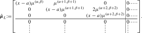
• (ii) The modified Sobolev orthogonality is neither diagonal nor symmetric. The matrix of measures takes the form of an upper bidiagonal matrix. For instance, with $\mathcalligra{n}=3$, the matrix $\hat{\varvec{\mu }}_L$ is given by:

  

• (iii) The monic polynomials $\hat{Q}^{(\alpha ,\beta )}_{1,l}$ are independent of $\mathcalligra{n}$; they represent the Christoffel perturbations of Jacobi polynomials corresponding to the measure $(x-a)(1-x)^\alpha (1+x)^\beta \textrm{d}x$. These polynomials satisfy Sobolev-type orthogonality relations:

  $$\begin{aligned} \begin{aligned}&\sum _{i=0}^{\mathcalligra{n}}\int _{-1}^1 \left( (x-a)\hat{Q}^{(\alpha ,\beta )}_{1,l}(x) \right) ^{(i)} (x^k)^{(i)}(1-x)^{\alpha +i}(1+x)^{\beta +i}\textrm{d}x =0, \\ {}&\qquad \quad l\in \{0,1,\dots ,k-1\}. \end{aligned} \end{aligned}$$

• (iv) Due to the fact that for the Jacobi polynomials $Q^{(\alpha ,\beta )}_l$ the Christoffel–Darboux formula (8) holds, we have

  $$\begin{aligned} \hat{Q}^{(\alpha ,\beta ,\mathcalligra{n})}_{1,l} (x)=h^{(\alpha ,\beta )}_l\dfrac{ K_{l}^{(\alpha ,\beta )}(x,a)}{Q^{(\alpha ,\beta )}_{l}(a)}. \end{aligned}$$

  Consequently, both perturbed biorthogonal SBPS are kernel polynomials, the first with respect to the Jacobi CD kernel and the second with respect to Jacobi–Sobolev CD kernel.

• (v) For the non-Sobolev case, the Christoffel perturbations of the squared norms are

  $$\begin{aligned} \hat{h}^{(\alpha ,\beta )}_l=\frac{Q^{(\alpha ,\beta )}{l+1}(a)}{Q^{(\alpha ,\beta )}_{l}(a)}h_l^{(\alpha ,\beta )}. \end{aligned}$$

  Therefore, the modified squared norms for the Sobolev orthogonality situation are given by:

  $$\begin{aligned} \hat{h}^{(\alpha ,\beta ,\mathcalligra{n})}_l= \hat{h}_l^{(\alpha ,\beta )}\sum _{i=0}^{\mathcalligra{n}}(l-i+1)_i(l+\alpha +\beta +1)_i. \end{aligned}$$

Definition 5.10

We introduce the $(2M+1)$ banded matrices

$$\begin{aligned} \begin{aligned} \hat{\omega }_L\hat{\Omega }_R&{:}{=} \hat{J}_{1,LR},&\hat{\omega }_R\hat{\Omega }_L&{:}{=} \hat{J}_{2,RL}. \end{aligned} \end{aligned}$$

We point out that a generalization of the notion of recurrence relation can be realized by allowing an intertwining of SBPS associated with different measure matrices, instead of using the same one.

Proposition 5.11

The right and left deformed SBPS satisfy the following $(2M+1)$ the relations

$$\begin{aligned} \begin{aligned} \hat{J}_{1,LR}\hat{P}_{R,1}(x)&=R(x)\hat{P}_{L,1}(x),&\hat{J}_{2,RL}\hat{P}_{L,2}(x)&=R(x)\hat{P}_{R,2}(x), \end{aligned} \end{aligned}$$

with

$$\begin{aligned} \hat{J}_{1,LR}=\hat{H}_L\hat{J}_{2,RL}^{\top }\hat{H}_R^{-1}. \end{aligned}$$

Observe that if $\varvec{\mu }\in \varvec{\mu }_{x}$, then there would be no distinction between L and R sequences. In addition, if we choose R(x) to be a polynomial of degree one, then $\hat{\omega } \cdot \hat{\Omega }$ is a $2(1)+1$-diagonal matrix and the standard three term recurrence relation is re-obtained.

5.2 Geronimus-Sobolev transformations

Let us now focus on the class of Geronimus transformations. To this aim, a polynomial $Q(x){:}{=} \prod _{i=1}^{s}(x-q_i)^{n_i}=Q_0+Q_1x+\dots +Q_{N-1}x^{N-1}+x^N$ of degree $\sum _{i=1}^{s}n_i=N$ is needed in order to define the left and right transformed measure matrices. We introduce the following auxiliary matrix, related to the polynomial Q(x):

The right and left Geronimus–Sobolev deformed measure matrices and moment matrices are

Definition 5.12

For $\{ q_i\}_{i=1}^s\cap \Omega =\varnothing$, the Geronimus–Sobolev deformed measure matrices are defined to be

We introduce the following masses where $\xi ^{(i)}$ are the $n_i \times n_i$ matrices of free parameters

Proposition 5.13

The more general perturbed matrix of measures that satisfies the requirements of Definition 5.12 are

Proposition 5.14

The transformed measure matrices and associated moment matrices are related to the original ones by the formulas

$$\begin{aligned} \varvec{\mu }{:}{=} Q({X})\check{\varvec{\mu }}_L,&\qquad \varvec{\mu }{:}{=} \check{\varvec{\mu }}_RQ({X}^{\top }),&\qquad G=Q(\Lambda )G_{\check{\varvec{\mu }}_L},&\qquad G=G_{\check{\varvec{\mu }}_R}Q\left( \Lambda ^{\top } \right) . \end{aligned}$$

The latter proposition and the assumption that the transformed moment matrices are LU-factorizable motivate the definition of the resolvents in terms of the following matrices.

Definition 5.15

We introduce the matrices

$$\begin{aligned} \check{\omega }_L&{:}{=} \check{H}_L \check{S}_{1,L}^{-\top }Q(\Lambda ^{\top })S_1^{\top }H^{-1}=\check{S}_{2,L}S_{2}^{-1},\\ \check{\omega }_R&{:}{=} \check{H}_R \check{S}_{2,R}^{-\top }Q(\Lambda ^{\top })S_2^{\top }H^{-1}=\check{S}_{1,R}S_{1}^{-1}. \end{aligned}$$

The right-hand side expressions are derived from the LU factorization of both the transformed and non-transformed moment matrices. Notably, it can be observed that these equalities entail that the resolvents are lower uni-triangular matrices, featuring only N non-vanishing diagonals below the main diagonal. To be specific:

where $\check{\omega }_{k,k-N}=\frac{\check{h}_k}{h_{k-N}}$ for $k>N$ and $\check{\omega }_{k,k}=1$.

Proposition 5.16

The perturbed Geronimus—Sobolev polynomials and their corresponding second-kind functions are interconnected with the original ones through the following formulas:

$$\begin{aligned}&\begin{aligned} \check{\omega }_LP_2(x)&=\check{P}_{2,L}(x),&\check{\omega }_L C_2(x)&=Q(x)\check{C}_{2,L}(x)-\check{H}_L\check{S}_{1,L}^{-\top }\textbf{Q}\,\chi (x) , \end{aligned}\\&\begin{aligned} \check{\omega }_RP_1(x)&=\check{P}_{1,R}(x),&\check{\omega }_R C_1(x)&=Q(x)\check{C}_{1,R}(x)-\check{H}_R\check{S}_{2,R}^{-\top }\textbf{Q}\,\chi (x). \end{aligned} \end{aligned}$$

Proof

The connection formulas for the polynomials are straightforward to derive, recalling their definition in terms of the factorization matrices and considering the definition of $\check{\omega }$. Conversely, the connection formulas for the second-kind functions follow as a consequence of the former, as we are about to demonstrate. We will present the proof for the right transformation, and it’s worth noting that the proof for the left transformation relies on similar ideas.

Firstly, let’s introduce the following definition and present a result that can be easily verified:

$$\begin{aligned} \Delta Q(x,y){:}{=} Q(x)-Q(y),&\quad \chi (x)^{\top }\textbf{Q} \,\chi (y)=-\frac{\Delta Q(x,y)}{y-x}. \end{aligned}$$

Using this result the next chain of equalities can be followed

$\square$

Let us now study the deformations of Christoffel–Darboux kernels.

Proposition 5.17

The deformed Christoffel–Darboux kernels are related to the original ones by means of the formulas

$$\begin{aligned} \check{K}_R^{[k]}(x,y)&=Q(x)K^{[k]}(x,y)- \begin{bmatrix}\check{P}_{2,R,k}(x)&\cdots&\check{P}_{2,R,k+N-1}(x) \end{bmatrix}\\&\quad \times \begin{bmatrix} \check{h}_{R,k}^{-1} &{} &{} \\ &{} \ddots &{} \\ &{} &{}\check{h}_{R,k+N-1}^{-1} \end{bmatrix} \begin{bmatrix} (\check{\omega }_R)_{k,k-N} &{} \cdots &{} (\check{\omega }_R)_{k,k-1} \\ &{} \ddots &{} \vdots \\ &{} &{}(\check{\omega }_R)_{k+N-1,k-1} \end{bmatrix} \begin{bmatrix} P_{1,k-N}(y) \\ P_{1,k+1-N}(y) \\ \vdots \\ P_{1,k-1}(y) \end{bmatrix},\\ \check{K}_L^{[k]}(x,y)&=Q(y)K^{[k]}(x,y)-\begin{bmatrix}\check{P}_{1,L,k}(x)&\cdots&\check{P}_{1,L,k+N-1}(x) \end{bmatrix}\\&\quad \times \begin{bmatrix} \check{h}_{L,k}^{-1} &{} &{} \\ &{} \ddots &{} \\ &{} &{}\check{h}_{L,k+N-1}^{-1} \end{bmatrix} \begin{bmatrix} (\check{\omega }_L)_{k,k-N} &{} \cdots &{} (\check{\omega }_L)_{k,k-1} \\ &{} \ddots &{} \vdots \\ &{} &{}(\check{\omega }_L)_{k+N-1,k-1} \end{bmatrix} \begin{bmatrix} P_{2,k-N}(x) \\ P_{2,k+1-N}(x) \\ \vdots \\ P_{2,k-1}(x) \end{bmatrix}. \end{aligned}$$

Similarly, the mixed kernels $k \ge N$ are related as follows

Proof

These expressions are a direct consequence of the connection formulas. $\square$

We shall also introduce a couple of useful matrices, which will be relevant in the subsequent discussion.

Definition 5.18

Let us introduce

and define the $N \times N$ matrices

where

$$\begin{aligned} \Xi _{R,j}{:}{=}\mathring{\xi }_R^{(j)}\eta _j \begin{bmatrix} \frac{Q_j^{(0)}(q_j)}{0!} &{}\frac{Q_j^{(1)}(q_j)}{1!}&{} \dots &{}\frac{Q_j^{(n_j-2)}(q_j)}{(n_j-2)!} &{} \frac{Q_j^{(n_j-1)}(q_j)}{(n_j-1)!} \\ 0 &{}\frac{Q_j^{(0)}(q_j)}{0!}&{} &{} &{}\frac{Q_j^{(n_j-2)}(q_j)}{(n_j-2)!}\\ \vdots &{} \ddots &{}\ddots &{} &{} \vdots \\ &{} &{} &{}\ddots &{}\frac{Q_j^{(1)}(q_j)}{1!} \\ 0 &{} \cdots &{} &{} 0 &{}\frac{Q_j^{(0)}(q_j)}{0!} \end{bmatrix} \\ \end{aligned}$$

and

$$\begin{aligned} \Xi _{L,j}{:}{=} \left( \mathring{\xi }^{(j)}_L\right) ^{\top } \eta _{j} {\begin{bmatrix} \frac{Q_j^{(0)}(q_j)}{0!} &{}\frac{Q_j^{(1)}(q_j)}{1!}&{} \dots &{}\frac{Q_j^{(n_j-2)}(q_j)}{(n_j-2)!} &{} \frac{Q_j^{(n_j-1)}(q_j)}{(n_j-1)!} \\ 0 &{}\frac{Q_j^{(0)}(q_j)}{0!}&{} &{} &{}\frac{Q_j^{(n_j-2)}(q_j)}{(n_j-2)!}\\ \vdots &{} \ddots &{}\ddots &{} &{} \vdots \\ &{} &{} &{}\ddots &{}\frac{Q_j^{(1)}(q_j)}{1!} \\ 0 &{} \cdots &{} &{} 0 &{}\frac{Q_j^{(0)}(q_j)}{0!} \end{bmatrix}}. \end{aligned}$$

An interesting characterization of the class of Geronimus-type transformed polynomials can be obtained in terms of quasi-determinants, as clarified by the following:

Theorem 5.19

For $k\ge N$, the Geronimus–Sobolev transformed polynomials are expressed in terms of the original polynomials via the formulas for the R objects

and for L objects

Proof

We shall focus on the case of right transformations. We start looking at the Geronimus transformed second kind functions

Therefore, multiplying the previous expression by Q(y) and letting $y\rightarrow q_j$, we obtain the Taylor expansion

$$\begin{aligned} Q(y)\check{C}_{1,R,k}(y)&= \begin{bmatrix}\frac{\check{P}_{1,R,k}^{(0)}(q_j)}{0!}&\frac{\check{P}_{1,R,k}^{(1)}(q_j)}{1!}&\dots&\frac{\check{P}_{1,R,k}^{(n_j-1)}(q_j)}{(n_j-1)!} \end{bmatrix} \Xi _{R,j} \begin{bmatrix} 1 \\ y-q_j\\ \vdots \\ (y-q_j)^{n_j-1} \end{bmatrix}\\&\quad +O(y-q_j)^{n_j}. \end{aligned}$$

The previous reasoning can be repeated for each j. Consequently, collecting all the information in the same matrix we can write the relation

$$\begin{aligned} \Pi _q[Q\check{C}_{1,R,k}]=\Pi _q[\check{P}_{1,R,k}]\Xi _R. \end{aligned}$$

By using the connection formula for the second kind functions, and applying $\Pi _q$ to both sides, if we also take into account the previous relation, we get the equations

$$\begin{aligned} \check{\omega }_R\Pi _q[C_1]&=\Pi _q[Q\check{C}_{1,R}]-\check{H}_R\check{S}_{2R}^{-\top }\textbf{Q}\Pi _q[\chi (x)],\\ \check{\omega }_R\Pi _q[C_1]&=\Pi _q[\check{P}_{1,R}]\Xi _R-\check{H}_R\check{S}_{2R}^{-\top }\textbf{Q}\Pi _q[\chi (x)]. \end{aligned}$$

Rearranging terms and using the connection formula for the polynomials, we arrive at the expression

$$\begin{aligned} \check{\omega }_R\left( \Pi _q[C_1]-\Pi _q[P_1]\Xi _R \right)&=-\check{H}_R\check{S}_{2R}^{-\top }\textbf{Q}\Pi _q[\chi (x)]. \end{aligned}$$

For $k\ge N$, this result can be made more explicit once written in the form

$$\begin{aligned} \begin{bmatrix}(\check{\omega }_R)_{k,k-N}&\dots&(\check{\omega }_R)_{k,k-1}&1 \end{bmatrix} \left( \Pi _q\begin{bmatrix} C_{1,k-N} \\ C_{1,k-N+1} \\ \vdots \\ C_{1,k} \end{bmatrix}- \Pi _q\begin{bmatrix} P_{1,k-N} \\ P_{1,k-N+1} \\ \vdots \\ P_{1,k} \end{bmatrix}\Xi _R \right)&=0, \end{aligned}$$

whence, the expression for the first right-family and their norms follows straightforwardly. In order to obtain the expression for the second right-family, a similar approach can be used, based now on the relations between CD kernels and their mixed versions. $\square$

Example: Geronimus perturbation of Jacobi–Sobolev polynomials. When we choose $q = x - a$ for a not belonging to the support of the original measures $\textrm{d}\mu _{i,j}$, for $l \in \mathbb {N}_0$, the resulting formulas are as follows:

$$\begin{aligned} \check{P}_{1,l}(x)&= P_{1,l}(x)-\dfrac{C_{1,l}(a)-\xi P_{1,l}(a)}{C_{1,l-1}(a)-\xi P_{1,l-1}(a)}P_{1,l-1}(x),\\ \check{h}_l&=-\dfrac{C_{1,l}(a)-\xi P_{1,l}(a)}{C_{1,l-1}(a)-\xi P_{1,l-1}(a)}h_{l-1},\\ \check{P}_{2,l} (x)&=h_{l-1}\dfrac{C_{1,l}(a)-\xi P_{1,l}(a)}{(C_{1,l-1}(a)-\xi P_{1,l-1}(a))^2} \left( (x-a) \left( 1+\mathcal {K}_2^{[l]}(x,a)-\xi K^{[l]}(x,a)]\right) \right) . \end{aligned}$$

Especially, for the Sobolev–Jacobi inner product defined in (4), where $a \notin [-1,1]$, and for $l \in \mathbb {N}_0$, we obtain:

$$\begin{aligned} \check{Q}^{(\alpha ,\beta ,\mathcalligra{n})}_{1,l}(x)&= Q^{(\alpha ,\beta )}_{l}(x)-\dfrac{C^{(\alpha ,\beta ,\mathcalligra{n})}_{l}(a)-\xi Q^{(\alpha ,\beta )}_{l}(a)}{C^{(\alpha ,\beta ,\mathcalligra{n})}_{l-1}-\xi Q^{(\alpha ,\beta )}_{l-1}(a)}Q^{(\alpha ,\beta )}_{l-1}(x),\\ \check{h}_l^{(\alpha ,\beta ,\mathcalligra{n})}&=-\dfrac{C^{(\alpha ,\beta ,\mathcalligra{n})}_{l}(a)-\xi Q^{(\alpha ,\beta )}_{l}(a)}{C^{(\alpha ,\beta ,\mathcalligra{n})}_{l-1}-\xi Q^{(\alpha ,\beta )}_{l-1}(a)}h^{(\alpha ,\beta ,\mathcalligra{n})}_{l-1},\\ \check{Q}^{(\alpha ,\beta ,\mathcalligra{n})}_{2,l} (x)&=h^{(\alpha ,\beta ,\mathcalligra{n})}_{l-1}\dfrac{C^{(\alpha ,\beta ,\mathcalligra{n})}_{l}(a)-\xi Q^{(\alpha ,\beta )}_{l}(a)}{\left( C^{(\alpha ,\beta ,\mathcalligra{n})}_{l-1}(a)-\xi Q^{(\alpha ,\beta )}_{l-1}(a)\right) ^2} \\&\quad \times \left( (x-a) \left( 1+\mathcal {K}^{(\alpha ,\beta ,\mathcalligra{n})}_{2,l-1}(x,a)-\xi K^{(\alpha ,\beta ,\mathcalligra{n})}_{l-1}(x,a)\right) \right) . \end{aligned}$$

Some observations follow:

• (i) These polynomials adhere to the following biorthogonal relations:

  $$\begin{aligned} \sum _{i=0}^{\mathcalligra{n}} \int _{-1}^{1} \frac{\textrm{d}^i \check{Q}^{(\alpha ,\beta ,\mathcalligra{n})}_{1,l}}{\textrm{d}x^i}\frac{\textrm{d}^i\left( (x-a)^{-1}\check{Q}^{(\alpha ,\beta ,\mathcalligra{n})}_{2,k}\right) }{\textrm{d}x^i} (1-x)^{\alpha +i}(1+x)^{\beta +i}\textrm{d}x=\delta _{l,k}\check{h}^{(\alpha ,\beta ,\mathcalligra{n})}_l. \end{aligned}$$

• (ii) The function $C^{(\alpha ,\beta )}_{l}(z)$ exhibits analyticity for $z\notin [-1,1]$, and by extension, in accordance with (10), so does $C^{(\alpha ,\beta ,\mathcalligra{n})}_{l}$. Consequently, the coefficients defined as

  $$\begin{aligned} c_l(a){:}{=} \frac{C^{(\alpha ,\beta ,\mathcalligra{n})}_{l}(a)}{Q^{(\alpha ,\beta )}_l(a)} \end{aligned}$$

  are well-defined.

  In light of this, by choosing the mass term such that $\xi \notin \{c_l(a)\}_{l=0}^\infty$, we establish that perturbed polynomials can be constructed.

• (iii) Note that $\check{\mu }_R$ is presently a lower triangular matrix, with entries representing the Jacobi-type measures multiplied by inverse powers of $(x-a)$. There is a potential mass term $\xi \delta (x-a)$ in the $\check{\mu }_{0,0}$ entry. To illustrate, for $\mathcalligra{n}=3$, we have:

  

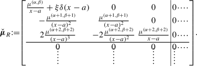
  Thus, while the original Sobolev orthogonality is diagonal, the Geronimus-perturbed version is neither diagonal nor symmetric.

We shall conclude this section with an observation on the recurrence relations for Geronimus-type polynomials arising from our transformation approach.

Definition 5.20

Let us define the following matrices

$$\begin{aligned} \check{J}_{1,RL}{:}{=} \check{S}_{1,R}Q(\Lambda )\check{S}_{1,L}^{-1} ,&\check{J}_{2,LR}{:}{=} \check{S}_{2,L}Q(\Lambda )\check{S}_{2,R}^{-1}. \end{aligned}$$

Proposition 5.21

The matrices $\check{J}_{1RL}$ and $\check{J}_{2LR}$ possess a $2N+1$ diagonal structure and are related to each other according to the formulas

$$\begin{aligned} \check{J}_{1R,L} \check{H}_L=\check{H}_R \check{J}_{2,LR}^{\top }. \end{aligned}$$

These induce a left and right $2N+1$ term recurrence relation involving the Geronimus transformed polynomials:

$$\begin{aligned} \check{J}_{1,RL}\check{P}_{1,L}=Q(x)\check{P}_{1,R},&\check{J}_{2,LR}\check{P}_{2,R}=Q(x)\check{P}_{2,L}. \end{aligned}$$

Proof

The proposition is a consequence of the relation

$$\begin{aligned} Q(\Lambda ) \check{G}_L&=\check{G}_R Q(\Lambda ^{\top }) \end{aligned}$$

combined with a LU-factorization of the moment matrices. $\square$

6 Conclusions and outlook

We have introduced an extensive class of Sobolev bi-orthogonal polynomial sequences derived from a moment matrix featuring an LU factorization. These sequences are associated with a measure matrix that defines the Sobolev bilinear form. Additionally, we have presented a theory of deformations for Sobolev bilinear forms, with a specific focus on additive Uvarov perturbations and polynomial deformations of the measure matrix. Notably, we introduce the concepts of Christoffel–Sobolev and Geronimus–Sobolev transformations. We explicitly determine the Christoffel-type formulas between these newly introduced polynomial sequences and existing ones in terms of quotients of determinants, in the line done for standard orthogonality in [34]. We have chosen the Jacobi–Sobolev polynomials [9] as a case study to demonstrate the impact of Uvarov, Christoffel, and Geronimus perturbations in the simplest scenarios.

It is noteworthy that in [12, 13], the authors derive differential equations for Laguerre–Sobolev and Jacobi–Sobolev types, assuming that the discrete parts are supported at the ends of the interval. This leads to the bispectrality of such polynomials. On a different note, as indicated in [14], a connection exists between Sobolev-type and standard matrix orthogonal polynomials. However, an intriguing open question remains: does a similar theory exist for the additive Uvarov perturbations discussed in Section 4.1?

When $\varvec{\mu }$ is a symmetric matrix of measures, the study of polynomials orthogonal with respect to the symmetric bilinear form $(f, h; \varvec{\mu }) = (f, h; P (X)WP (X^\top ))$ presents an intriguing perturbation of Christoffel type. This perturbation lies beyond the scope of the methods discussed in this manuscript, and its detailed analysis remains an open problem to be explored in future work.

References

Alfaro, M., Marcellán, F., Rezola, M.L., Ronveaux, A.: Sobolev-type orthogonal polynomials: the nondiagonal case. J. Approx. Theory 83, 266–287 (1995)
Althammer, P.: Eine Erweiterung des Orthogonalitätsbegriffes bei Polynomen und deren Anwendung auf die beste Approximation. J. Reine Angew. Math. 211, 192–204 (1962)
Álvarez Fernández, C., Ariznabarreta, G., Garcia-Ardila, J.C., Mañas, M., Marcellán, F.: Christoffel transformations for matrix orthogonal polynomials in the real line and the non-Abelian 2D Toda lattice hierarchy. Int. Math. Res. Not. 5, 1285–1341 (2017)
Ariznabarreta, G., García-Ardila, J.C., Mañas, M., Marcellán, F.: Non-Abelian integrable hierarchies: matrix biorthogonal polynomials and perturbations. J. Phys. A: Math. Theor. 51, 205204 (2018)
Ariznabarreta, G., García-Ardila, J.C., Mañas, M., Marcellán, F.: Matrix biorthogonal polynomials on the real line: Geronimus transformations. Bull. Math. Sci. 9, 1950007 (2019)
Ariznabarreta, G., García-Ardila, J.C., Mañas, M., Marcellán, F.: Uvarov Perturbations for Matrix Orthogonal Polynomials. arXiv:2312.05137 (2023)
Ariznabarreta, G., Mañas, M.: Matrix orthogonal matrix polynomials on the unit circle and Toda type integrable systems. Adv. Math. 264, 396–463 (2014)
Barrios Rolania, D., López Lagomasino, G., Pijeira Cabrera, H.: The moment problem for a Sobolev inner product. J. Approx. Theory 100, 364–380 (1999)
Ciaurri, Ó., Mínguez Ceniceros, J.: Fourier series of Jacobi–Sobolev polynomials. Integral Transforms Spec. Funct. 30(4), 334–346 (2019)
Christoffel, E.B.: Über die Gaussische Quadratur und eine Verallgemeinerung derselben. J. Reine Angew. Math. 55, 61–82 (1858). (in German)
Durán, A.J.: A generalization of Favard’s theorem for polynomials satisfying a recurrence relation. J. Approx. Theory 74, 83–109 (1993)
Durán, A.J., de la Iglesia, M.D.: Differential equations for discrete Laguerre–Sobolev orthogonal polynomials. J. Approx. Theory 195, 70–88 (2015)
Durán, A.J., de la Iglesia, M.D.: Differential equations for discrete Jacobi–Sobolev orthogonal polynomials. J. Spectr. Theory 8, 191–234 (2018)
Durán, A.J., Van Assche, W.: Orthogonal matrix polynomials and higher-order recurrence relations. Linear Algebra Appl. 219, 261–280 (1995)
Evans, W.D., Littlejohn, L.L., Marcellán, F., Markett, C., Ronveaux, A.: On recurrence relations for Sobolev orthogonal polynomials. SIAM J. Math. Anal. 26, 446–467 (1995)
Geronimus, J.: On polynomials orthogonal with regard to a given sequence of numbers and a theorem by W. Hahn. Izv. Akad. Nauk SSSR 4, 215–228 (1940). (in Russian)
Golinskii, L.: On the scientific legacy of Ya. L. Geronimus (to the hundredth anniversary), in Self-Similar Systems (Proceedings of the International Workshop (July 30–August 7, Dubna, Russia, 1998)), 273–281, Edited by V.B. Priezzhev and V. P. Spiridonov, Publishing Department, Joint Institute for Nuclear Research, Moscow Region, Dubna
Iserles, A., Koch, P.E., Norsett, S.P., Sanz Serna, J.M.: On polynomials orthogonal with respect to certain Sobolev inner products. J. Approx. Theory 65, 151–175 (1991)
Ismail, M.E.H.: Classical and Quantum Orthogonal Polynomials in One Variable. Cambridge University Press, Cambridge (2005)
Kim, H.K., Kwon, K.H., Littlejohn, L.L., Yoon, G.J.: Diagonalizability and symmetrizability of Sobolev-type bilinear forms: a combinatorial approach. Linear Algebra Appl. 460, 111–124 (2014)
Koekoek, R.: The search for differential equations for certain sets of orthogonal polynomials. J. Comput. Appl. Math. 49, 111–119 (1993)
Kwon, K.H., Littlejohn, L.L., Yoon, G.J.: Ghost matrices and a characterization of symmetric Sobolev bilinear forms. Linear Algebra Appl. 431, 104–119 (2009)
Marcellán, F., Moreno-Balcázar, J.J.: Asymptotics and zeros of Sobolev orthogonal polynomials on unbounded supports. Acta Appl. Math. 94, 163–192 (2006)
Marcellán, F., Pérez-Valero, M.F., Quintana, Y., Urieles, A.: Recurrence relations and outer relative asymptotics of orthogonal polynomials with respect to a discrete Sobolev type inner product. Bull. Math. Sci. 4, 83–97 (2014)
Marcellán, F., Petronilho, J.C.: Orthogonal polynomials and coherent pairs: the classical case. Indag. Math. 3, 287–307 (1995)
Marcellán, F., Szafraniec, F.H.: A matrix algorithm towards solving the moment problem of Sobolev type. Linear Algebra Appl. 331, 155–164 (2001)
Marcellán, F., Xu, Yuan: On Sobolev orthogonal polynomials. Expo. Math. 33, 308–352 (2015)
Meijer, H.G.: A short history of orthogonal polynomials in a Sobolev space. I. The non-discrete case. 31st Dutch Mathematical Conference (Groningen, 1995). Nieuw Arch. Wisk. (4) 14(1), 93–112 (1996)
Meijer, H.G.: Determination of all coherent pairs. J. Approx. Theory 89, 321–343 (1997)
Olver, P.J.: On multivariate interpolation. Stud. Appl. Math. 116, 201–240 (2006)
Pijeira Cabrera, H.E.: Teoría de Momentos y Propiedades Asintíticas para Polinomios Ortogonales de Sobolev. Doctoral Dissertation, Universidad Carlos III de Madrid (1998)
Schäfke, F.W.: Zu den Orthogonalpolynomen von Althammer. J. Reine Angew. Math. 252, 195–199 (1972)
Schäfke, F.W., Wolf, G.: Einfache verallgemeinerte klassische Orthogonal polynome. J. Reine Angew. Math. 262(263), 339–355 (1973)
Zhedanov, A.: Rational spectral transformations and orthogonal polynomials. J. Comput. Appl. Math. 85, 67–86 (1997)
Acknowledgements
The authors would like to express their gratitude for the diligent work of the reviewer. Their observations, remarks, and suggestions have significantly enhanced the legibility and clarity of this paper. The research of M.M. has received support from the Spanish “Agencia Estatal de Investigación” research project PID2021-122154NB-I00, titled Orthogonality and Approximation with Applications in Machine Learning and Probability Theory. G.A. also expresses gratitude to the Program "Ayudas para Becas y Contratos Complutenses Predoctorales en España", Universidad Complutense de Madrid, Spain. The research of P.T. has been supported by the research project PGC2018-094898-B-I00, MINECO, Spain, and by the ICMAT Severo Ochoa Programme for Centres of Excellence in R &D (CEX2019-000904-S), Ministerio de Ciencia, Innovación y Universidades, Spain. P.T. is a member of the Gruppo Nazionale di Fisica Matematica (INDAM), Italy. The authors express gratitude to the anonymous reviewer whose insightful suggestions have significantly enhanced the readability and clarity of the paper.
Funding
Open Access funding provided thanks to the CRUE-CSIC agreement with Springer Nature.
Author information
Authors and Affiliations
Contributions
All the authors wrote the paper and reviewed it. G.A. had a determinant role in the development of this project.
Corresponding author
Ethics declarations
Conflict of intersts
The authors declare that they have no competing interests.
Ethical approval
Not applicable.
Additional information
Publisher's Note
Springer Nature remains neutral with regard to jurisdictional claims in published maps and institutional affiliations.
Rights and permissions
Open Access This article is licensed under a Creative Commons Attribution 4.0 International License, which permits use, sharing, adaptation, distribution and reproduction in any medium or format, as long as you give appropriate credit to the original author(s) and the source, provide a link to the Creative Commons licence, and indicate if changes were made. The images or other third party material in this article are included in the article’s Creative Commons licence, unless indicated otherwise in a credit line to the material. If material is not included in the article’s Creative Commons licence and your intended use is not permitted by statutory regulation or exceeds the permitted use, you will need to obtain permission directly from the copyright holder. To view a copy of this licence, visit http://creativecommons.org/licenses/by/4.0/.
About this article
Cite this article
Ariznabarreta, G., Mañas, M. & Tempesta, P. Sobolev orthogonal polynomials, Gauss–Borel factorization and perturbations. Anal.Math.Phys. 14, 89 (2024). https://doi.org/10.1007/s13324-024-00883-5
Received:
Revised:
Accepted:
Published:
DOI: https://doi.org/10.1007/s13324-024-00883-5