
Abstract
The inherently stochastic nature of community detection in real-world complex networks poses an important challenge in assessing the accuracy of the results. In order to eliminate the algorithmic and implementation artifacts, it is necessary to identify the groups of vertices that are always clustered together, independent of the community detection algorithm used. Such groups of vertices are called constant communities. Current approaches for finding constant communities are very expensive and do not scale to large networks. In this paper, we use binary edge classification to find constant communities. The key idea is to classify edges based on whether they form a constant community or not. We present two methods for edge classification. The first is a GCN-based semi-supervised approach that we term Line-GCN. The second is an unsupervised approach based on image thresholding methods. Neither of these methods requires explicit detection of communities and can thus scale to very large networks of the order of millions of vertices. Both of our semi-supervised and unsupervised results on real-world graphs demonstrate that the constant communities obtained by our method have higher F1-scores and comparable or higher NMI scores than other state-of-the-art baseline methods for constant community detection. While the training step of Line-GCN can be expensive, the unsupervised algorithm is 10 times faster than the baseline methods. For larger networks, the baseline methods cannot complete, whereas all of our algorithms can find constant communities in a reasonable amount of time. Finally, we also demonstrate that our methods are robust under noisy conditions. We use three different, well-studied noise models to add noise to the networks and show that our results are mostly stable.
1 Introduction
Detecting communities is a fundamental operation in large-scale real-world networks. Unfortunately, this operation is also inherently stochastic. The communities detected can vary based on the algorithm, the parameters, and even the order in which the vertices are processed. One method to reduce the effect of these algorithmic artifacts is to identify constant communities. Constant communities are a group of vertices which are always assigned to the same community and thus exhibit stable partitions. In Fig. 1, the first two rows represent the community structure from two different algorithms, and the third row shows the constant communities that are common across the two results.
Current approaches to detecting constant communities involve executing a community detection algorithm multiple times, or running different community detection algorithms, and then combining the results to identify the set of vertices that are grouped together across all the runs. These approaches are, however, very expensive in terms of time and memory and do not scale to large networks. In this paper, we propose binary edge classification as a method to identify constant communities. The edges of a network are classified as whether or not they are part of a constant community. Since the classification depends only on easily computable properties of edges and not on finding communities, our methods are much faster and can be applied to very large networks.
Our contribution Our primary contributions are as follows;
-
Applying semi-supervised methods, namely the Graph Convolution Network (GCN) (Kipf and Welling 2017), to implement binary classification of edges. Since GCN is typically used for classifying nodes, we convert the graph into a line graph where each edge becomes a node (see Fig. 2).
-
Applying unsupervised methods based on image thresholding (namely bi-level dos Anjos and Reza Shahbazkia 2008, histogram concavity Rosenfeld and De La Torre 1983, Binary Otsu and TSMO aka Multi-Otsu Otsu 1979) to implement binary classification. We create a histogram of the values of the features, and then classify the edges based on the thresholds in the histogram (see Fig. 3).
-
We evaluate the accuracy and performance of our methods with two baseline approaches: CHAMP (Weir et al. 2017) and the Consensus community algorithm (Aditya et al. 2019). Our experiments demonstrate that our proposed methods provide comparable or higher accuracy, as per F1-score or normalized mutual information (NMI). For medium and large networks, the baseline methods do not complete, but all our methods finish at a reasonable time.
-
Studying the effect of noise with respect to our approaches. Over three different noise models (Uniform, Crawled, and Censored), we show that our methods provide high accuracy, even when noise is introduced.

Example of constant communities. Different colors (red and green) represent different communities to which vertices are assigned for each type of algorithm. Constant communities are the clusters that occur across all the outputs

Steps to detect the constant community using semi-supervised workflow. In Step 1, the line graph is generated from the input graph. In Step 2, features are extracted from the original graph. In Step 3, the feature vector for each node in the line graph is constructed using the features in Step 2. In Step 4, the dimensions of the feature vectors are reduced using PCA. In Step 5, with the help of the selected training nodes, GCN is applied to the line graph to classify the nodes. Finally, the edges of the input graph are classified using the classified nodes in the line graph to find the constant community

Steps to detect the constant community using unsupervised workflow. In Step 1, features are extracted using the neighbors of each edge. In Step 2, histograms are generated for each feature. In Step 3, by applying an image thresholding algorithm, an optimum threshold is obtained for each histogram. In Step 5, edges are filtered out based on the thresholds, and finally we get the constant communities
The present paper is an extension of our previous work (Chowdhury et al. 2021) published in the Proceedings of the ASONAM 2021 conference. In the earlier work, we only studied an unsupervised approach to detecting constant community while considering only the variants of the classic Otsu’s image thresholding algorithm to filter out the constant community edges. In this paper, we consider both the semi-supervised and unsupervised approaches to obtaining constant community. In the semi-supervised approach, we have used GCN and Line graph of the input graph to detect the constant community. In the unsupervised approach, in addition to Otsu’s algorithm, we also study the bi-level and histogram concavity methods for better generalization in thresholding. We have also added the study on noisy environment to the present work, and have empirically demonstrated that our method still performs better than the baselines.
This paper is organized as follows: In Sect. 2, we provide an overview of the semi-supervised and unsupervised methods used for our algorithms. In Sect. 3, we describe how we use these algorithms to find constant communities. In Sect. 4, we present the experimental results that demonstrate the advantages of our approach, as well as how our methods perform in a noisy setting. We present related work in Sect. 5, reproducibility in Sect. 6, and conclude with a discussion of future directions in Sect. 7.
2 Overview of the methods
In this section, we describe the different semi-supervised and unsupervised methods that we used for binary classification of edges.
2.1 Semi-supervised classification
We use graph convolutional network (GCN) (Kipf and Welling 2017) as our semi-supervised technique. Since GCN is a node-based classifier and we are doing an edge classification task, we convert our graph G to its corresponding line graph (Frank and Z 1960) L. A brief description of the line graph and the GCN is given as follows.
-
Line graph The line graph L(\(V_l\), \(E_l\)) (Frank and Z 1960) of a graph G(V, E) can be defined as follows:
-
Each vertex \(u_l\) in L represents an edge e in G.
-
(\(u_l, v_l\)) \(\in E_l\) iff the edges \(e_u\) and \(e_v\) in G representing \(u_l\) and \(v_l\), respectively, are incident in G.
A toy example of the construction of the line graph is given in Fig. 4. We can obtain the number of nodes and edges in a line graph easily. The number of nodes in a line graph L is \(\vert V_l \vert = \vert E \vert\) and the number of edges in L is \(\vert E_l \vert = \frac{1}{2}\sum _{i=1}^{\vert V \vert }deg_{i}^{2} - \vert E \vert\), where \(deg_i\) is the degree of vertex \(v_i \in V\). Conversion of a graph G to its line graph L can be done in linear time (Lehot 1974; Roussopoulos 1973).
Fig. 4 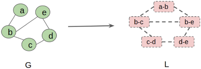
Construction of the line graph L from the graph G. Edges in G are converted to nodes in L
-
-
GCN The Graph Convolutional Neural Network (GCN) (Kipf and Welling 2017) is a type of Graph Neural Network (GNN) used for semi-supervised node classification on graphs. It is a first-order approximation of the Spectral Graph Convolution (Hammond et al. 2011). Formally, the GCN can be described as the following equation:
$$\begin{aligned} H^{k+1} = {\sigma }(\hat{A}H^{k}W^{k}) \end{aligned}$$where \(\hat{A} = \tilde{D}^{-0.5}\tilde{A}\tilde{D}^{-0.5}\), \(\tilde{A} = A + I\), I be the identity matrix of order \(\vert V \vert \times \vert V \vert\). \(\tilde{D} = \sum _j\tilde{A}_{ij}\), A be the adjacency matrix of the undirected graph G of size \(\vert V \vert \times \vert V \vert\), \(\sigma\) is the activation function (e.g., \(ReLU(\cdot ) = max\{0,\cdot \}\)), \(H^{k}\) is the feature representation at layer k; \(H^{0} = X = [x_1, x_2, ..., x_n]^{T} \in {\mathbb {R}}^{\vert V \vert \times c}\) be the feature matrix, \(x_i \in {\mathbb {R}}^{c}\) be the feature vector of dimension c and \(W^{{k}}\) is the weight matrix at layer k. In the output layer, the softmax function can be used as the activation function to classify the nodes in the graph.
Fig. 5 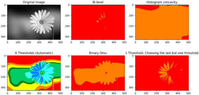
Various image thresholding techniques that delineate the foreground of an image from its background


2.2 Unsupervised classification
In our unsupervised method, we use some popular image thresholding algorithms such as bi-level (dos Anjos and Reza Shahbazkia 2008), Binary Otsu Otsu (1979), Multi-Otsu Huang and Wang (2009), and histogram concavity (Rosenfeld and De La Torre 1983).
2.2.1 Bi-level thresholding
A histogram is perfectly balanced if it has the same distribution of background and foreground. In bi-level thresholding method, an unbalanced histogram is tried to balance to find out the optimum threshold. It assumes that the input image is divided into two main classes: (i) the background and (ii) the foreground.
-
Formal overview Let m(g) be the number of entries having feature value g, L be the number of feature values, \(e_{0}\) and \(e_{L-1}\) be the first and last feature values (along the x-axis) in the histogram. So, \(e_{mid} = \frac{e_{0}+e_{L-1}}{2}\) be the middle of these two feature values. Now, the weight of the left side of the \(e_{mid}\) be \(W_{l} = \sum _{i=e_{0}}^{e_{mid}-1}m(i)\) and the right side would be \(W_{r} = \sum _{i=e_{mid}}^{e_{L-1}}m(i)\). Based on the proposed algorithm in dos Anjos and Reza Shahbazkia (2008) (Algorithm 4.1), it checks which side is heavier and update \(W_l\), \(W_r\), \(e_{0}\) and \(e_{L-1}\) accordingly until \(e_{0}\) = \(e_{L-1}\) = T = optimum threshold.
2.2.2 Binary Otsu
Otsu’s binary classification (Otsu 1979) is used to binarize grayscale images such that the object in the foreground can be distinguished from the background. The output is a single intensity threshold that separates pixels into two classes: foreground and background. To determine this optimal threshold, the algorithm adjusts the threshold values to maximize the variance in intensity between the two classes.
-
Formal overview The probability distribution of g is, \(p(g) = m(g)/m\); m is the total number of entries. For a threshold T, all entries with feature value below T are given by \(n_{B}(T) = \sum _{i=e_{0}}^{t}p(i)\) and all entries with feature value over the threshold are given by \(n_{O}(T) = \sum _{i=T}^{e_{L-1}}p(i)\). \(e_{i}\) is the \(i^{th}\) feature value, L is the number of the feature values, \(t \in \{e_{0}, ..., e_{L-1}\}\) is the maximum value just below T.
Let \(\mu _{B}(T)\) be the mean, and \(\sigma _{B}^{2}(T)\) be the variance of all entries with feature value less than the threshold, which in this case is analogous to the background of the image. Let \(\mu _{O}(T)\) be the mean, and \(\sigma _{O}^{2}(T)\) be the variance of all entries with feature value above the threshold, which in this case is analogous to the foreground, i.e., the object present in the image. Let \(\sigma ^{2}\) is the combined variance and \(\mu\) is the combined mean over all edges. Given these values, the within class variance can be defined as \(\sigma _{W}^{2}(T) = n_{B}(T)\sigma _{B}^{2}(T) + n_{O}(T)\sigma _{O}^{2}(T)\) and between class variance can be defined as; \(\sigma _{X}^{2}(T) = \sigma ^{2} - \sigma _{W}^{2}(T) = n_{B}(T)n_{O}(T)[\mu _{B}(T) - \mu _{O}(T)]^{2}\).
We apply Otsu’s method to obtain T such that \(\sigma _{X}^{2}(T)\) is maximized. However, as shown in Fig. 5, the single threshold-based binarization may not always yield the best results. In this case, the flower (object) cannot be demarcated from the background by the conventional Binary Otsu.
2.2.3 Multi-Otsu
Otsu’s binary-level thresholding (Otsu 1979) can be extended to multi-level thresholding (Huang and Wang 2009) in order to determine a number of thresholds to segment an image into clusters and recognize the various parts of it. Fig. 5 provides an example of an image segmentation task using multi-level Otsu thresholding.
We have used the Two-Stage Multi-threshold Otsu algorithm (TSMO) (Huang and Wang 2009; Huang and Lin 2011). Our goal was to see if, from among the multiple thresholds, we might judiciously arrive at one that better demarcates the object and the background as compared to the Binary Otsu. Clearly, this improves the result over that of Binary Otsu in Fig. 5.
-
Formal overview In multi-level thresholding, if a graph is segmented into K clusters (\(C_0, C_1, ..., C_{K-1}\)) then we need to look for \(K-1\) thresholds. The histogram of L values of a given feature is divided into \(M (> (K-1))\) groups. So, L can be written as \(\bigcup \nolimits _{q=0}^{M-1} L_{q}\), where each \(L_{q}\) is a non-empty subset of L and \(L_{q1} \cap L_{q2} = \phi\), where \(q1 \not = q2\) and \(q1, q2 \in \{0,...,M-1\}\). The occurrence probability \(P_{L_{q}}\) and the mean feature value \(M_{L_{q}}\) of \(L_{q}\) can be written as \(P_{L_{q}} = \sum _{i \in L_{q}}p(i) \text { and } M_{L_{q}} = \frac{\sum _{i \in L_{q}} i*p(i)}{ P_{L_{q}}}\). Therefore, for each cluster, \(C_{k}\), where \(k \in \{0,... K-1\}\), the cumulative probability \(w_{k} = \sum _{L_{q} \in C_{k}}P_{L_{q}}\) and mean feature value \(\mu _{k} = \sum _{L_{q} \in C_{k}}\frac{M_{L_{q}}*P_{L_{q}}}{w_{k}}\). Hence, the mean feature value of the whole graph \(\mu = \sum _{k=0}^{K-1}\mu _{k}w_{k}\) and between class variance \(\sigma ^{2}_{B} = \sum _{k=0}^{K-1}w_{k}(\mu _{k} - \mu )^{2}\). In the first stage of TSMO, Multi-level Otsu thresholding is used to find the optimal sets with number \(\{q_{0}^{*}, q_{1}^{*}, ..., q_{K-2}^{*}\)} for which \(\sigma ^{2}_{B}\) is maximum; Formally, \(\{q^{*}_{0}, q^{*}_{1},..., q^{*}_{K-2}\}\) = \({{\,\mathrm{arg\,max}\,}}_{e_{0}\le q_{0}< q_{1}...<q_{K-2}<M-1}\{\sigma ^{2}_{B}(q_{0}, q_{1},..., q_{K-2})\}\). Hence, optimal thresholds fall into \(\{ L_{q_{0}^{*}}, L_{q_{1}^{*}}, ..., L_{q_{K-2}^{*}}\}\). In the second stage, the optimal threshold \(th^{*}_{k}\) for each group \(L_{q_{k}^{*}}\) is computed using the Binary Otsu thresholding as \(th^{*}_{k} = {{\,\mathrm{arg\,max}\,}}_{th_{k} \in L_{q_{k}^{*}}}\{\sigma ^{2}_{B}(th_{k})\}\), \(k = 0, 1, ..., K-2\), finding the optimal threshold \(th^{*}_{k}\) for which \(\sigma ^{2}_{B}\) is maximum.
2.2.4 Histogram concavity analysis
For a histogram of an image, the ranges can be easily separated iff the image can be clearly segmented into object and background. In this case, the valley can be easily seen and the threshold is the point at the bottom of the valley. But when the ranges overlap, then there are no valleys in the histogram. In that case, the optimum threshold could be found at the root of the shoulder (where the object peak and background pick overlap). Finding the valleys and the shoulders is not a trivial task. But both of them are part of the concavities in the histogram. By analyzing the concavity structure, one can find the optimum threshold.
-
Formal overview We can see a histogram H as a 2-D bounded region as: (\(e_{0}, 0\)), (\(e_{0}, m(e_{0})\)), (\(e_{L-1}, m(e_{L-1})\)) and (\(e_{L-1}, 0\)). By constructing the convex hull of H, we can find the concavity of H. A convex hull \(\bar{H}\) of H is the smallest convex polygon that contains H. The concavity can be measured by the set difference \(H - \bar{H}\). To construct \(\bar{H}\), we start from (\(e_{0}, m(e_{0})\)) compute the slope \(\theta _{i}\) between points (\(e_{0}, m(e_{0})\)) and (\(e_{i}, m(e_{i})\)) for \(1 \le i < L\). So, (\(e_{0}, m(e_{0})\)), (\(e_{k_1}, m(e_{k_1})\)) be the side of the convex hull if \(\theta _{k_1}\) be the largest among the slopes. This process will be repeated, i.e., we find the slope of (\(e_{k_1}, m(e_{k_1})\))(\(e_{i}, m(e_{i})\)), \(k_2+1 \le i < L\) and \(\theta _{k_2}\) be the largest slope yielding (\(e_{k_1}, m(e_{k_1})\))(\(e_{k_2}, m(e_{k_2})\)) and so on, until we reach \(L-1\).
Let \(\bar{m}(e_{i})\) be the height of \(\bar{H}\) at property value \(e_{i}\). A point \(e_{i}\) is in a concavity if (\(\bar{m}(e_{i})\) - \(m(e_{i})\)) \(> 0\). Optimum thresholds can be found at \(e_{t}\) for which (\(\bar{m}(e_{t})\) - \(m(e_{t})\)) is maximum.
-
Example An example of how the optimum threshold can be found using histogram concavity is provided in Fig. 6. In Fig. 6(a), we can see a histogram H. In Fig. 6(b) to 6(f), the construction of the convex hull \(\bar{H}\) of H is shown. Fig. 6(f) shows the convex hull \(\bar{H}\) of H along with H. In Fig. 6(g), we scan from left to right and compute \(\bar{m}(e_{i})\) - \(m(e_{i})\), \(\forall i \in \{0, 1, ..., L-1\}\), and finally, a value \(e_t\) is found for which (\(\bar{m}(e_{t})\) - \(m(e_{t})\)) is maximum. Therefore \(e_t\) is chosen as the optimum threshold.
Fig. 6 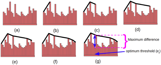
Finding the optimum threshold using histogram concavity. Fig. a denotes the histogram H constructed using the feature values and their frequencies. Figs. b to f represent the construction of the convex hull \(\bar{H}\) over H (represented by black lines). In Fig. g, a point \(e_t\) is found for which the difference between \(\bar{m}(e_{t})\), the frequency of \(e_t\) in \(\bar{H}\) and \(m(e_{t})\), the frequency of \(e_t\) in H is maximum

3 Our contribution
We first propose a semi-supervised edge classification method for constant community identification. We also propose an unsupervised edge classification task for the same purpose. In both of our classification methods, we find the constant communities by transforming the problem to a binary classification of edges.
3.1 Semi-supervised edge classification method
In the semi-supervised (graph-based) technique, we only know a few node labels, and the goal is to predict the labels of other nodes. A popular deep learning approach that uses graph-based semi-supervised learning techniques is GCN. GCN is primarily used to classify the nodes in a graph.
In our work, we use the GCN for the edge classification task and find constant communities. To enable the GCN to classify the edges, we convert the input graph to its corresponding line graph. In this way, each edge in the input graph is represented by a unique node in its corresponding line graph. Finally, the classification of nodes in the line graph implies the classification of edges in the input graph.
A schematic diagram of how this approach works is provided in Fig. 2 . Details of the key steps are given as follows:
-
Step 1: Line graph generation By default, GCN is a node classifier. So, to make the GCN work as an edge classifier, we first convert the input graph G to its corresponding line graph L, and then we classify the nodes in the line graph. Since each node in the line graph L represents an edge in the input graph G, classifying the nodes in L is the same as classifying the edges in G.
-
Step 2: Feature generation from the input graph One of the requirements to classify the nodes in L is to have a feature vector for each node. Each feature vector comprises a sequence of features. In this step, we will discuss the generation of the features required to construct a feature vector.
The likelihood that an edge will always be within a community is determined by the connections between the neighbors of the endpoints. To classify the edges in G, we select several features that indicate that the neighbors of the endpoints and the endpoints themselves form dense clusters. Since an edge e in G represents a node \(u_{le}\) in L, therefore, constructing features for \(e \in E\) is the same as constructing features for \(u_{le} \in V_l\).
We extracted the features of an edge \(e = (u, v)\) in G based on four methods that use the neighbors of u and v to create four vectors of features, viz., \(F_{EI}(e)\), \(F_{EU}(e)\), \(F_{NI}(e)\), and \(F_{NU}(e)\). Each element in the vectors represents a feature. The construction of these four vectors is given below:
-
(i)
\(F_{EI}(e)\): For each edge e, we generate a vector \(F_{EI}(e)\) of size \(\vert E \vert\) while initializing each cell to zero. Note that each cell represents an edge in G and hence a node in L. Then, we collect the set of common edges \(EI_{e}\) between the neighbors of the two terminals of the edge e. We then mark those cells in the vector to 1, corresponding to the edges in \(EI_{e}\).
-
(ii)
\(F_{EU}(e)\): For each edge e, we create a vector \(F_{EU}(e)\) of size \(\vert E \vert\) while initializing each cell to zero. Note that each cell represents an edge in G and hence a node in L. Then, we collect the union of edges \(EU_{e}\) between the neighbors of the two terminals of the edge e. We then mark those cells in the vector to 1, corresponding to the edges in \(EU_{e}\).
-
(iii)
\(F_{NI}(e)\): For each edge e, we create a vector \(F_{NI}(e)\) of size \(\vert V \vert\) while initializing each cell to zero. Note that each cell represents a node in G. Then, we collect the set of common nodes \(NI_{e}\) between the neighbors of the two terminals of the edge e. We then mark those cells in the vector to 1 corresponding to the nodes in \(NI_{e}\).
-
(iv)
\(F_{NU}(e)\): For each edge e, we create a vector \(F_{NU}(e)\) of size \(\vert V \vert\) while initializing each cell to zero. Note that each cell represents a node in G. Then, we collect the set of union of nodes \(NU_{e}\) between the neighbors of the two terminals of the edge e. We then mark those cells in the vector to 1, corresponding to the nodes in \(NU_{e}\).
-
(i)
-
Step 3: Feature vector generation for the line graph Let \(F(u_{le})\) represent the feature vector of a node \(u_{le} \in V_l\). We can write \(F(u_{le})\) as F(e), where F(e) represents the feature vector of the edge (corresponding to \(u_{le}\)) in V. F(e) is constructed by horizontally concatenating four vectors: \(F_{EI}(e)\), \(F_{EU}(e)\), \(F_{NI}(e)\), and \(F_{NU}(e)\).
Therefore the length of the feature vector F(e) and hence \(F(u_{le})\) will be: \(\vert E \vert\) + \(\vert E \vert\) + \(\vert V \vert\) + \(\vert V \vert\).
-
Step 4: Dimension reduction of the feature vectors The length of the feature vector is too large for a large graph, which causes an increase in the training time of the GCN. Therefore we reduce the dimension of the feature vector to 20 by applying Principle Component Analysis (PCA) (Karl 1901).
-
Step 5: Training nodes selection and applying GCN.
-
(a)
Training nodes selection Since semi-supervised learning requires a set of known label nodes for its training purpose, we run a particular community detection algorithm a few times (2 - 3 times) on G and select two sets of edges: (a) edges that always belong to the same community \(E_{C}\) and (b) edges that do not belong to any particular community \(E_{NC}\) for all runs. We then label the nodes in L corresponding to edges in \(E_{C}\) to 1, constructing the node set \(V_{Cl} \subset V_l\), and the nodes in L corresponding to edges in \(E_{NC}\) to 0, constructing the node set \(V_{NCl} \subset V_l\). The set of training nodes is thus: \(V_{Tl} = V_{Cl} \cup V_{NCl}\).
-
(b)
Applying GCN for node classification After generating the feature vectors and selecting the training nodes, we apply GCN to L. GCN classifies the node set \(V_l\) into two classes: \(V_{l1}\) and \(V_{l0}\). The edges in G representing the nodes in \(V_{l1}\) denote the set of constant community edges and the edges in G representing the nodes in \(V_{l0}\) denote the set of non-constant community edges.
-
(a)
3.2 Unsupervised edge classification methods
Although the semi-supervised approach performs well, it has some drawbacks. (i) It needs a set of training nodes (known labeled nodes) and obtaining a sufficient number of training nodes can be difficult; (ii) Generation of line graph is time and memory consuming; (iii) Training a large line graph is also time-consuming. In order to deal with these problems, we tried a novel unsupervised approach. In this approach, we find four local properties of each edge with the help of the neighbors of its two terminals and generate a histogram for each of these properties. Then, using a popular image thresholding algorithm, we find optimum thresholds for each histogram. Finally, we plug these thresholds into our novel Algorithms 1 and 2 to filter out the edges in the graph and generate the constant communities. A schematic diagram of how this approach works is provided in Fig. 3. Our unsupervised approach consists of the following key steps:
-
Step 1: Extracting the features for each edge For a vertex u, let N(u) denote the set of neighbors; \(\Delta (u)\) denotes the set of triangles containing vertex u; Also, for a vertex set Y, let \(\Gamma (Y)\) denote the density of the subgraph that is induced by the nodes in Y, i.e., the ratio of the number of edges in the subgraph to the total possible edges in the subgraph. To classify these edges, we compute four features (see Fig. 7) as follows:
-
Subgraph density induced by both u and v’s neighbors ( \(D_{both}\)). Formally, \(D_{both}(u,v)=\Gamma (N(v) \cap N(u))\).
-
Subgraph density caused by u and v, as well as their neighbors ( \(D_{any}\)). Formally, \(D_{any}(u,v)=\Gamma (N(v) \cup N(u))\).
-
The Proportion of triangles containing both u and v to triangles containing at least one of u or v. (\(D_{tri}\)). Formally, \(D_{tri}(u,v)=\frac{\vert \Delta (u) \cap \Delta (v) \vert }{\vert \Delta (u) \cup \Delta (v) \vert }\).
-
The Jaccard index of u and v’s neighbors ( JI). Formally, \(JI(u,v)=\frac{\vert N(v)\cap N(u) \vert }{\vert N(v) \cup N(u)\vert }\).
Fig. 7 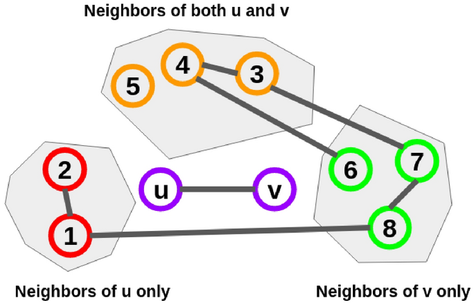
Features used for edge classification. For an edge (u, v); the red vertices are connected to u only, the green vertices are connected to v only, and the orange vertices are connected to u and v both. For ease of visualization, the connections to u and v are not shown.
\(D_{both}(u,v)\) = density of (3, 4, 5) = \(\frac{1}{3}\) \(D_{any}(u,v)\) = density of \((1,2,3,4,5,6,7,8,u,v) = \frac{18}{45}\) \(D_{tri}(u,v) = \vert \{(u,v,3),(u,v,4),(u,v,5)\} \vert \div \vert \{(u,v,3),(u,v,4),(u,v,5), (u,1,2),(u,3,4),\) \((v,7,8),(v,4,6),(v,3,7),(v,3,4) \} \vert = \frac{1}{3}\) JI(u, v) = \(\vert \{3,4,5\} \vert \div \vert \{1,2,3,4,5,6,7,8,u,v\}\vert\) = \(\frac{3}{10}\)
-
-
Step 2: Formation of histograms We create a histogram for each of the features (the x-axis has values; the y-axis has frequency). We named the histograms as \(H_{any}, H_{both}, H_{tri}\), and \(H_{JI}\), corresponding to \(D_{any}, D_{both}, D_{tri}\), and JI, respectively.
-
Step 3: Obtaining threshold using image thresholding algorithm In this step, we obtain an optimum threshold for each of the histograms. We use a popular image thresholding algorithm to obtain these thresholds: \(T_{any}, T_{both}, T_{tri}\) and \(T_{JI}\) correspond to \(H_{any}, H_{both}, H_{tri}\) and \(H_{JI}\), respectively.
-
Step 4: Filtering the edges Suppose B100 denotes the set that contains the edges that always belong to a community, and B0 denotes the rest of the edges that may or may not belong to some community. The following conditions hold for an edge to be classified as B100:
-
(i)
JI is high, i.e., it has a high percentage of common neighbors, and also, \(D_{both}\) is high, i.e., the density of the subgraph induced by the common neighbors is high.
-
(ii)
\(D_{any}\) is high, i.e., the subgraph induced by all the neighbors of u and v (including u and v) has a high density.
-
(iii)
\(D_{tri}\) is high, which means the proportion of triangles containing both u and v to triangles containing at least one of u or v is high. Since many triangles are supported by an edge, it is very likely that their terminals are co-clustered.
-
(i)

3.2.1 Variants of Image thresholding algorithm for edge classification
In Step 3 of the above unsupervised approach, we used two variants of thresholding algorithm: (i) binary-thresholding and (ii) multi-thresholding. In addition to this, we also studied two modifications of the multi-thresholding approach to obtain better output.
-
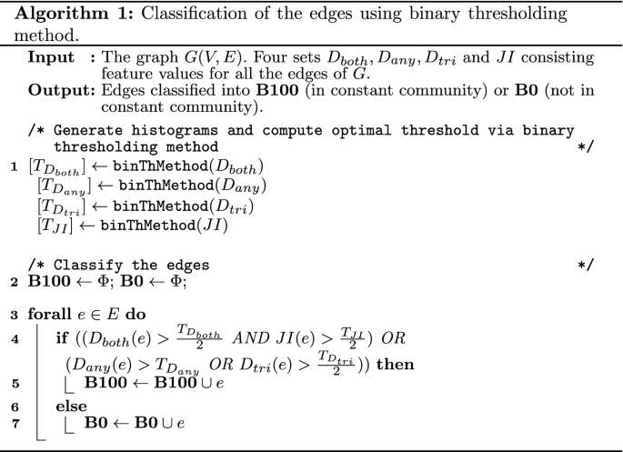
Edge classification using binary-thresholding algorithm (Algorithm 1). In the binary classification algorithm, an optimal threshold for each histogram is separately found and the results are combined for the classification of the edges as per the rules in Step 4 above. We define a high value of the features as being higher than the threshold given by the corresponding thresholding algorithm. We used three variants of binary-thresholding approaches viz; bi-level, histogram concavity, and Binary Otsu in our study.
-
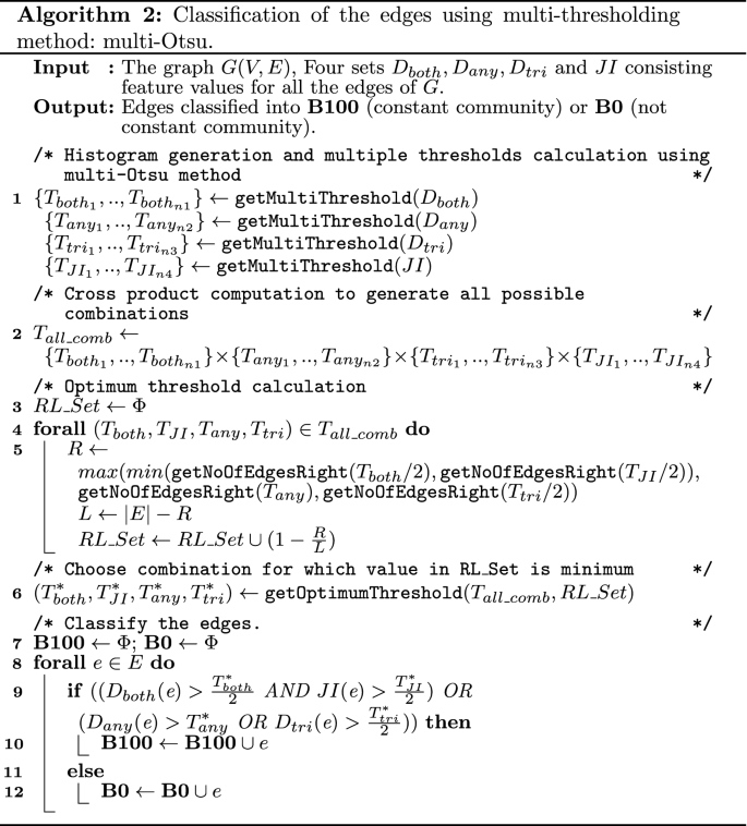
Edge classification using multi-thresholding algorithm (Algorithm 2). We used TSMO (henceforth called Multi-Otsu) as the multi-thresholding algorithm to find the optimum thresholds. The main challenge in applying Multi-Otsu is that once the set of thresholds is generated, all the possible combinations of the thresholds and features have to be tested to find the optimal one. For example, if the Multi-Otsu algorithm returns k different thresholds, then with 4 features, \({\mathcal {O}}(k^{4})\) combinations should be checked. Checking each edge’s property against all these thresholds is computationally expensive.
To make classification computationally feasible, we consider the thresholds for each feature separately rather than in combination. For each threshold, we compute how many edges are to the right (i.e., are higher) than the threshold and how many edges are to the left (i.e., are lower) than the threshold. Given a strong community structure, the number of edges within communities should be at least as much as the number of edges across communities – if not higher. Therefore, as a first cut, we identify the threshold that produces an almost equal number of edges on the left (lower) and right (higher) sides. This optimal threshold gives us the initial set of edges that will always be within communities.
-
Modification 1: Using iterative multi-thresholding We further improve the accuracy of Algorithm 2 by iteratively applying Multi-Otsu on the subgraph induced by the edges in B0, which can potentially contain more within community edges.
We recompute the histograms for the edges in B0 based on the feature values of only these edges. Using Algorithm 2, we find the optimal threshold on this set and obtain a split of B0 into B0’ and B100’ where the assumptions for B0’ and B100’ are the same as for B0 and B100, respectively. We then move the edges of B100’ into B100 and set B0 to B0’
This iteration is continued until the change in threshold is very low(\(\le\) \(\delta\), where we set \(\delta\) = 0.01) and no new edges move from B0 to B100. We named this method Multi-Otsu iterative.
-
Modification 2: Fixing the singleton communities Once the edges in B100 have been classified, i.e., they are always within a community, the subgraph induced by the edges in B100 forms the constant communities. However, as seen in the case of the blue vertex in Fig. 1, some communities may be composed of just one vertex, i.e., form singleton communities.
Most community detection algorithms do not retain singleton communities and absorb this vertex into a neighboring community. We identify nodes that are not part of the constant communities. If the node (vertex) has degree 2, then, if both of its neighbors belong to the same community, we put the node into that community. If the neighbors are in different communities, then we move the node to one of those communities, since there is a 50% chance that at least one of them will be included in one of the two communities. We named this method Multi-Otsu iterative+SC.
We have seen empirically that this heuristic produces a slightly higher F1-score. However, the accuracy decreases as the heuristic is applied to vertices of a higher degree. This is because if the vertex was classified as a singleton, then it could be in any of its neighboring communities. The probability that the vertex is in a certain community decreases with the number of neighboring communities.
-
To summarize, we present multiple heuristics to classify edges that form constant communities. First, we study the semi-supervised method where we convert a graph G to its corresponding line graph L. By classifying the nodes in the line graph L using GCN, we classify the edges in the input graph G to obtain the edges that are possible candidates for constant communities. Then, we discuss the pitfalls of the semi-supervised approach, which includes the problem of obtaining the training set and time and memory requirements. After that, we discuss some unsupervised approaches where we use different local neighborhood properties and generate histograms based on these properties. This is followed by applying a popular image thresholding algorithm to find the optimum threshold in the histogram. After the generation of the threshold for each histogram, we apply certain rules based on the combination of these thresholds to filter out the constant community edges. In our unsupervised approach, we use both binary and multi-thresholding algorithms. We use several variants of binary-thresholding algorithms like bi-level, histogram concavity, and Binary Otsu. In our multi-thresholding algorithm, we use the extended version of Binary Otsu’s (Multi-Otsu) algorithm. To improve the results, we applied two modifications to the Multi-Otsu method: (i) Multi-Otsu iterative, where we apply the Multi-Otsu method to the predicted non-constant community edges set, and (ii) Multi-Otsu iterative+SC, where we take care of the singleton communities.


4 Empirical results
In this section, we present our experimental setup and the results from these experiments.
4.1 Experimental setup
-
Datasets and Ground Truth A set of real-world networks are used for our work (Table 1). We obtain ground truth constant community by executing a community detection 50 times. The order of the vertices is permuted at each execution. As shown in Chakraborty et al. (2013), changing the order in which vertices are processed changes the results. The communities that were common to all of these runs were designated as the constant community ground truth for the given community detection method.
We used three community detection algorithms: Louvain Blondel et al. (2008), Infomap Rosvall and Bergstrom (2008), and Label Propagation Raghavan et al. (2007) to create the ground truth for the small-sized networks.
For medium-sized (nodes = 10K+ and edges in the range of 10K+ to 1M+) and large-sized networks (nodes = 1M+ and edges in the range of 1M+ to 10M+), it is very expensive to run a community detection algorithm multiple times. Therefore, we used only the Louvain method (which is faster than the other two methods) for the ground truth creation.
Table 1 The test suite of real-world networks -
Specifics of the classification algorithms For the semi-supervised method, we used GCN to classify the nodes in the line graph (and hence the edges in the corresponding graph). For this GCN model, we use Optuna Akiba et al. (2019) for hyper-parameter tuning. The list of hyper-parameters, we used, can be found in Table 2. We have used 15% training nodes from both classes. To measure the F1-scores, we have used all the nodes in the network.
For the unsupervised methods, we implemented bi-level, histogram concavity, and Otsu’s thresholding (both Binary and Multi-Otsu) algorithms.
Table 2 The list of hyper-parameters used in Optuna -
Baselines methods We use two baseline algorithms to compare with our method. The first method is the consensus community algorithm presented in Aditya et al. (2019). This involves forming a consensus matrix D based on multiple (we selected 100) executions of community detection, where \(D_{ij}\) represents the number of times vertices i and j were co-clustered in the same community. A community detection algorithm is iteratively applied to the weighted graphs formed from the consensus matrices until less than a convergence percent (default value of 2%) of all nonzero entries in \(D_i\) have weights of less than one.
The second method is called CHAMP (Convex Hull of Admissible Modularity Partitions) (Weir et al. 2017). Given a set of partitions, CHAMP identifies the modularity optimization for each partition to obtain the subset of partitions that are potentially optimal while discarding the other partitions. These baseline methods can typically handle only one type of community detection algorithm at a time. For equitable comparison, we also compared our classification algorithms with a fixed community detection method.
-
Implementation details We implemented the algorithms in python (version 3.6). Code to implement Multi-Otsu can be found in George (2019). The codes for the baseline methods, consensus community and CHAMP, are at (Tandon et al. 2019) and (Weir et al. 2017), respectively. All algorithms were run on an IntelXeon(R) Processor with CPU E3-1270 V2, 3.50GHz8, and 128 GB of memory.
4.2 Comparisons among various methods
We compared both our proposed semi-supervised ((i) Line-GCN) and unsupervised methods; ((ii) bi-level; (iii) histogram concavity; (iv) Binary Otsu; (v) multi-level Otsu thresholding (Multi-Otsu); (vi) iterative multi-level Otsu thresholding (Multi-Otsu iterative); (vii) Multi-Otsu iterative+SC) with the baseline methods Consensus and CHAMP. Since the baselines are stochastic, the average results from several runs are reported.
-
Comparison of F1-scores with the ground truth communities In our results, B100 holds the set of constant community edges. We compared the set B100 with the set of edges in the constant communities that are obtained from the ground truth.
Figs. 8, 9, and 10 depict the results (F1-score) for the small-sized networks. Fig. 11 shows the results for the medium and large-sized networks. In Figs. 8, 9, and 10, the ground truth community edges are obtained by executing the Louvain, Infomap, and Label propagation algorithms, respectively, whereas in Fig. 11, only the Louvain algorithm is used to obtain the ground truth community edges.
For the few small networks (Jazz, Email, and Polbooks) and all the large networks, the semi-supervised (Line-GCN) approach gives the maximum F1-score. For the few networks like Jazz, Email, Com-amazon, Com-Youtube, and Com-liveJ, the bi-level thresholding approach gives poor performance. Other binary and multi-thresholding methods performed well in most of the networks. Compared to the baselines, our methods, especially Line-GCN, histogram concavity, Binary Otsu, Multi-Otsu, and its variants, exhibit better results in most cases. For medium- and large-scale networks, baseline methods (not shown in Fig. 11) were not completed within a reasonable time (i.e., within 2 days) except for the co-authorship network (F1-scores = 70%).
-
NMI comparison with the ground truth communities How well are the predicted constant communities overlapped with the ground truth constant communities? To know that, we construct the constant communities from the edges in B100 by obtaining the connected components. After that, the normalized mutual information (NMI) is computed between the set of predicted constant communities and the set of ground truth communities. As we can see in Table 3, our results are giving comparable or better NMI scores than the baselines. More specifically, for the small-sized networks, in most cases (except for the Football graph), Line-GCN gives comparable scores (second best or best) to the baselines. The unsupervised approach gives the worst performance in Jazz and Email networks, but in other cases, this approach gives the best or second-best performance. For all the medium and large-sized graphs, both the semi-supervised (Line-GCN) and the unsupervised approaches (especially the Multi-Otsu iterative with singleton community) perform well. Both methods give equally good results for Com-amazon and Wiki-topcats networks. For Com-dblp and Co-authorship networks, L-GCN gives the best result, whereas the unsupervised method gives the second best, and for the Com-Youtube network, the unsupervised method gives the best result, whereas L-GCN gives the second best.
-
Execution time Table 4 reports the time to compute ground truth constant communities, which increases to as much as 963 hours for the largest network. Thus, finding constant communities empirically is not feasible for large networks and an efficient algorithm of the like proposed in this paper is essential.
Table 5 shows the execution time for obtaining constant communities using our algorithms as well as the baselines for the small networks. Our unsupervised algorithms are ~ 10 times faster. For medium and large networks (see Table 5), our unsupervised algorithms are fast, even for networks with 10M+ nodes and 100M+ edges. Although sometimes the semi-supervised algorithms give comparable results to the unsupervised ones, it takes longer time. The baseline methods take either a long time to finish or do not finish within a feasible time frame.
Fig. 8 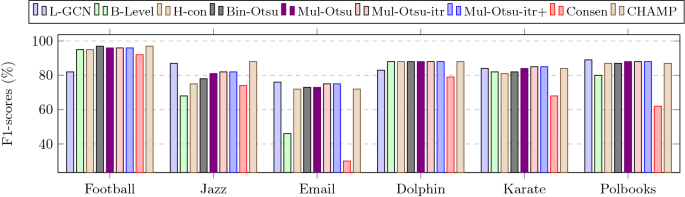
Performance of different methods for obtaining constant communities for small networks. The ground truth constant community edges are obtained by executing the Louvain algorithm. The abbreviated names are as follows; L-GCN: Line-GCN, B-Level: Bi-level, H-Con: Histogram concavity, Bin-Otsu: Binary Otsu, Mul-Otsu: Multi-Otsu, Mul-Otsu-itr: Multi-Otsu iterative, Mul-Otsu-itr+: Multi-Otsu iterative with singleton community, Consen: Consensus
Fig. 9 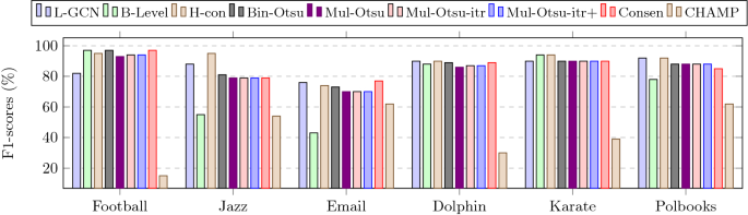
Performance of different methods for obtaining constant communities for small networks. The ground truth constant community edges are obtained by executing the Infomap algorithm. The abbreviated names are as follows; L-GCN: Line-GCN, B-Level: Bi-level, H-Con: Histogram concavity, Bin-Otsu: Binary Otsu, Mul-Otsu: Multi-Otsu, Mul-Otsu-itr: Multi-Otsu iterative, Mul-Otsu-itr+: Multi-Otsu iterative with singleton community, Consen: Consensus
Fig. 10 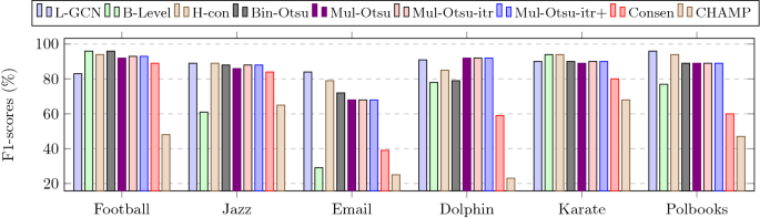
Performance of different methods for obtaining constant communities for small networks. The ground truth constant community edges are obtained by executing the Label propagation algorithm. The abbreviated names are as follows; L-GCN: Line-GCN, B-Level: Bi-level, H-Con: Histogram concavity, Bin-Otsu: Binary Otsu, Mul-Otsu: Multi-Otsu, Mul-Otsu-itr: Multi-Otsu iterative, Mul-Otsu-itr+: Multi-Otsu iterative with singleton community, Consen: Consensus
Fig. 11 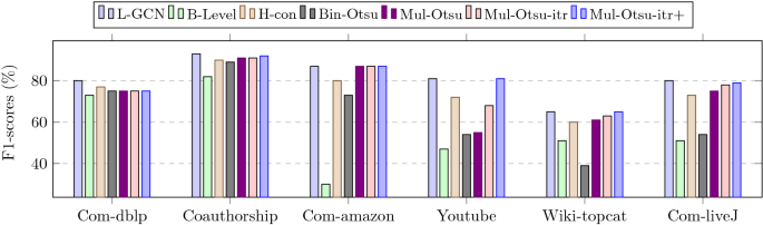
Performance of different methods for obtaining constant communities for medium and large networks. The ground truth constant community edges are obtained by executing the Louvain algorithm. The baselines are not shown here because they did not end within a sizable amount of time. Only for co-authorship network (not shown in the figure), the consensus method gives 70% F1-scores
Table 3 Comparison of NMI. Best results are highlighted in green, second-best results are highlighted in blue, and the worst in red. X: The process did not end within a sizable amount of time. L-GCN: Line-GCN Table 4 Time required for ground truth generation (#iterations = 50) Table 5 Time for identifying constant communities for all networks. Best timing performances for each dataset are denoted by green cells and the worst by red cells. X: The process did not end within a sizable amount of time. The abbreviated names are as follows; L-GCN: Line-GCN, B-Level: Bi-level, H-Con: Histogram concavity, Bin-Otsu: Binary Otsu, Mul-Otsu: Multi-Otsu, Mul-Otsu-itr: Multi-Otsu iterative, Mul-Otsu-itr+: Multi-Otsu iterative with singleton community, Consen: Consensus


4.3 Results under noisy domains
Real-world networks are often noisy and can be missing some edges. We use three noise models from Yan and Gregory (2011) as follows to test how well our method performs under noise.
-
Uniform: The edges are removed randomly and repeatedly until a certain number of edges remain.
-
Crawled: Starting from a node with the smallest maximum distance from all other nodes, use BFS to crawl the network and keep the required number of edges.
-
Censored: At each step, randomly choose one of the maximum degree nodes and then randomly delete one of its edges, until a certain number of edges remain in the network.
Because introducing noise into small networks causes them to disconnect, we only tested on larger networks. For each noise type and percentage of edges removed, we created the ground truth and computed the F1-score of our predicted edge labels. In Fig. 12, we show that even when the network is noisy, our method gives good accuracy.

F1-scores under different noise scenarios
5 Related work
5.1 Classification using Image Thresholding
We didn’t find any work where image thresholding algorithms are applied to detect communities or any graph-related problems. However, the image thresholding algorithms are very commonly used for classification of images such as Mahdy et al. (2020) where they use the image thresholding algorithms to classify detection of COVID-19 patients. Iqbal et al. (2018) presented a survey for the detection and classification of citrus plant diseases, and Amin et al. (2020) presented a method to detect and classify tumors. Survey papers by Garcia-Lamont et al. (2018), Asokan and Anitha (2019), and Chouhan et al. (2018) present an overview of all the works related to image thresholding algorithms for classifying images. This paper is the first attempt to use this approach for graph-related classification problems. We believe this approach will be extended to other classification problems in the future.
5.2 Graph neural networks
Graph Convolution Networks are categorized as a sub-class of techniques under the broader domain of Graph Neural Networks (GNNs). There are various types of GNNs based on their application domains. A graph neural network can be used in many fields, such as classifying the nodes (Kipf and Welling 2017; Hagenbuchner and Monfardini 2009), link prediction (Zhang and Chen 2018; Li et al. 2021), graph classification (Defferrard et al. 2016; Wu et al. 2022; Mueller et al. 2022), graph generation (Li et al. 2018; Liao et al. 2019; Hu et al. 2020), and community detection (Sun et al. 2021; Luo et al. 2021). A comprehensive survey on GNNs can be found here (Wu et al. 2019, 2020). Souravlas et al. (2021) gave a brief overview of current state& advances in deep learning techniques for community detection. We have also seen many attempts to detect communities using GNN such as Bruna and Li (2017), Shchur and Günnemann (2019), and Moradan et al. (2021). We didn’t find any work that has attempted to use GNN for detecting constant communities.
In recent studies, GNNs have also been used with line graphs. For example, a supervised community detection task using a GNN model called line graph neural network (LGNN) is proposed in Chen et al. (2017). LGNN uses both the graph G and its corresponding line graph L(G) to find the communities in G. Using the LGNN, the authors in Cai et al. (2021) study the link prediction task in the graph.
5.3 Constant or consensus community
Community detection is a well-studied problem and numerous algorithms exist (see survey el-Moussaoui et al. 2019). However, finding the non-stochastic communities is a much less studied and much more challenging problem.
Community detection algorithms are primarily based on optimizing objective functions. Due to underlying stochasticity, resulting structures show considerable variations. Riolo and Newman (2020) suggest that stochasticity can be reduced by identifying “building blocks,” i.e., groups of network nodes that are usually found together in the same community. In Chakraborty et al. (2013), a precursor of this work, the authors have investigated the properties of constant communities with respect to within community and across community edges.
A popular approach to finding stable communities is via consensus clustering as introduced in Lancichinetti and Fortunato (2012). Variations include multi-resolution consensus clustering (Jeub et al. 2018), ensemble clustering (Poulin and Théberge 2019; Chakraborty et al. 2016) and fast consensus (Aditya et al. 2019) clustering and CHAMP Weir et al. (2017). Nevertheless, as seen here, these are not yet fast enough for large networks.
6 Reproducibility
All our source code and implementations, including the baseline implementation, are available at https://github.com/anjangit000/ImgThAlgoConsComm. The URL provided above has a Readme file which explains the steps to reproduce the results presented in this paper. For large networks such as Com-Amazon, Com-Dblp, Youtube, and wiki-topcats, we recommend to use a HPC cluster with a minimum RAM of 128GB and Python parallel framework such as mpi4py (Dalcin and Fang 2021), and Dask (Rocklin 2015). The results can also be executed on non-HPC clusters, but it will take a long time for large networks.
7 Conclusions and future work
We applied the semi-supervised and the unsupervised classification techniques for identifying constant communities that scale to large networks. Although the semi-supervised approach gives good results, it requires training data, which is sometimes difficult to obtain. We also applied an image segmentation inspired unsupervised approach. We showed that the unsupervised approach gives results as good as the semi-supervised approach and in less time. Our work is an important contribution to stabilizing community detection results for large networks.
One of the important future works that we wish to take up is the detection of overlapping constant communities. Overlapping community detection requires grouping the nodes into clusters so that there exist some nodes that belong to more than one community; in other words, some nodes may have multiple community ID’s. In the overlapping constant communities, the nodes should maintain two properties, (i) they should always belong to the same overlapping community (s), and, (ii) nodes may have multiple labels. To identify the edges of the overlapping communities we have to explore which features are the most informative for classification. Another challenge for overlapping communities is the increased memory footprint as nodes can have multiple communities. To make our application scalable and handle large-scale graphs for detecting constant overlapping communities, we need to run this on distributed clusters. We plan to modify our data structure and use high-performance computing framework (HPC) such as MPI/Open ACC to implement the proposed algorithm and overlapping version.
Other future plans include applying the constant communities obtained using our method to design various downstream applications, including outlier detection, domain adaptation, feature selection, and other important problems in data mining. On the implementation side, we aim to develop a parallel version of our algorithms to further improve their performance.
References
Aditya T, Aiiad A, Vijey T, Wadee A, Santo F (2019) Fast consensus clustering in complex networks. Physical Review E. https://doi.org/10.1103/physreve.99.042301
Akiba T, Sano S, Yanase T, Ohta T, Koyama M (2019) Optuna: A next-generation hyperparameter optimization framework. In: Proceedings of the 25rd ACM SIGKDD International Conference on Knowledge Discovery and Data Mining
Amin J, Sharif M, Yasmin M, Fernandes SL (2020) A distinctive approach in brain tumor detection and classification using mri. Pattern Recogn Lett 139:118–127
Asokan A, Anitha J (2019) Change detection techniques for remote sensing applications: a survey. Earth Sci Inf 12(2):143–160
Blondel VD, Guillaume J-L, Lambiotte R, Lefebvre E (2008) Fast unfolding of communities in large networks. J. of Stat. Mech. (10), 10008
Bruna J, Li X (2017) Community detection with graph neural networks. stat 1050, 27
Cai L, Li J, Wang J, Ji S (2021) Line graph neural networks for link prediction. IEEE Transactions on Pattern Analysis and Machine Intelligence
Chakraborty T, Srinivasan S, Ganguly N, Bhowmick S, Mukherjee A (2013) Constant communities in complex networks. Sci Rep 3(1):1–9
Chakraborty T, Park N, Subrahmanian VS (2016). Ensemble-based algorithms to detect disjoint and overlapping communities in networks. https://doi.org/10.1109/ASONAM.2016.7752216
Chakraborty T, Srinivasan S, Ganguly N, Mukherjee A, Bhowmick S (2014) On the permanence of vertices in network communities., 1396–1405
Chen Z, Li X, Bruna J (2017) Supervised community detection with line graph neural networks. arXiv preprint arXiv:1705.08415
Chouhan SS, Kaul A, Singh UP (2018) Soft computing approaches for image segmentation: a survey. Multimed Tools Appl 77(21):28483–28537
Chowdhury A, Srinivasan S, Bhowmick S, Mukherjee A, Ghosh K (2021) Constant community identification in million scale networks using image thresholding algorithms. In: Proceedings of the 2021 IEEE/ACM International Conference on Advances in Social Networks Analysis and Mining. ASONAM ’21, pp. 116–120. Association for Computing Machinery, New York, NY, USA . https://doi.org/10.1145/3487351.3488350
Dalcin L, Fang Y-LL (2021) mpi4py: Status update after 12 years of development. Comput Sci Eng. https://doi.org/10.1109/MCSE.2021.3083216
Defferrard M, Bresson X, Vandergheynst P (2016) Convolutional Neural Networks on Graphs with Fast Localized Spectral Filtering
dos Anjos A, Reza Shahbazkia H (2008) Bi-level Image Thresholding - A Fast Method. In: Proceedings of the First International Conference on Bio-inspired Systems and Signal Processing - Volume 2: BIOSIGNALS, (BIOSTEC 2008), pp. 70–76 . https://doi.org/10.5220/0001064300700076. INSTICC
el-Moussaoui M, Agouti T, Tikniouine A, el Adnani M, (2019) A comprehensive literature review on community detection: approaches and applications. Procedia Comput Sci. https://doi.org/10.1016/j.procs.2019.04.042
Frank H, Z NR, (1960) Some properties of line digraphs. Rendiconti del Circolo Matematico di Palermo. https://doi.org/10.1007/BF02854581
Garcia-Lamont F, Cervantes J, López A, Rodriguez L (2018) Segmentation of images by color features: A survey. Neurocomputing 292:1–27
George P (2019) Improved two-stage multithreshold Otsu method. https://github.com/ps-george/multithreshold
Guimerà R, Danon L, Díaz-Guilera A, Giralt F, Arenas A (2003) Self-similar community structure in a network of human interactions. Phys Rev E. https://doi.org/10.1103/physreve.68.065103
Guimerà R, Danon L, Díaz-Guilera A, Giralt F, Arenas A (2003) Self-similar community structure in a network of human interactions. Phys Rev E. https://doi.org/10.1103/physreve.68.065103
Hagenbuchner FSMGACTM, Monfardini G (2009) The graph neural network model. Appl Netw Sci 20(1):61–80
Hammond DK, Vandergheynst P, Gribonval R (2011) Wavelets on graphs via spectral graph theory. Appl Comput Harmon Anal 30(2):129–150. https://doi.org/10.1016/j.acha.2010.04.005
Huang Deng-Yuan WCH, Ta-Wei Lin (2011) Automatic multilevel thresholding based on two-stage otsu’s method with cluster determination by valley estimation. Int J Innovative Comput, Inf Control 7(10):5631–5644
Huang D-Y, Wang C-H (2009) Optimal multi-level thresholding using a two-stage otsu optimization approach. Pattern Recogn Lett 30:275–284. https://doi.org/10.1016/j.patrec.2008.10.003
Hu Z, Dong Y, Wang K, Chang K-W, Sun Y (2020) Gpt-gnn: Generative pre-training of graph neural networks. In: Proceedings of the 26th ACM SIGKDD International Conference on Knowledge Discovery & Data Mining, pp. 1857–1867
Iqbal Z, Khan MA, Sharif M, Shah JH (2018) An automated detection and classification of citrus plant diseases using image processing techniques: a review. Comput and Electron Agric 153:12–32
Jeub L, Sporns O, Fortunato S (2018) Multiresolution consensus clustering in networks. Sci Rep. https://doi.org/10.1038/s41598-018-21352-7
Karl P (1901) On lines and planes of closest fit to systems of points in space. LIII. https://doi.org/10.1080/14786440109462720
Kipf TN, Welling M (2017) Semi-Supervised Classification with Graph Convolutional Networks. In: Proceedings of the 5th International Conference on Learning Representations. ICLR ’17 . https://openreview.net/forum?id=SJU4ayYgl
Lancichinetti A, Fortunato S (2012) Consensus clustering in complex networks. Sci Rep. https://doi.org/10.1038/srep00336
Lehot PGH (1974) An optimal algorithm to detect a line graph and output its root graph. J ACM 21(4):569–575. https://doi.org/10.1145/321850.321853
Leskovec J, Krevl A (2014) SNAP Datasets: Stanford Large Network Dataset Collection. http://snap.stanford.edu/data
Liao R, Li Y, Song Y, Wang S, Hamilton W, Duvenaud DK, Urtasun R, Zemel R (2019) Efficient graph generation with graph recurrent attention networks. Advances in Neural Information Processing Systems 32
Li Y, Vinyals O, Dyer C, Pascanu R, Battaglia P (2018) Learning Deep Generative Models of Graphs
Li B, Xia Y, Xie S, Wu L, Qin T (2021) Distance-enhanced graph neural network for link prediction. ICML 2021 Workshop on Computational Biology
Luo L, Fang Y, Cao X, Zhang X, Zhang W (2021) Detecting communities from heterogeneous graphs: A context path-based graph neural network model. In: Proceedings of the 30th ACM International Conference on Information & Knowledge Management, pp. 1170–1180
Mahdy LN, Ezzat KA, Elmousalami HH, Ella HA, Hassanien AE (2020) Automatic x-ray covid-19 lung image classification system based on multi-level thresholding and support vector machine. MedRxiv
Moradan A, Draganov A, Mottin D, Assent I (2021) Ucode: Unified community detection with graph convolutional networks. arXiv preprint arXiv:2112.14822
Mueller TT, Paetzold JC, Prabhakar C, Usynin D, Rueckert D, Kaissis G (2022) Differentially private graph classification with gnns. arXiv preprint arXiv:2202.02575
Otsu NA (1979) Threshold Selection Method from Gray-level Histograms. IEEE Transa Sys, Man and Cybernetics 9(1):62–66. https://doi.org/10.1109/TSMC.1979.4310076
Poulin V, Théberge F (2019) Ensemble clustering for graphs: comparisons and applications. Appl Netw Sci 4(1):51
Raghavan UN, Albert R, Kumara S (2007) Near linear time algorithm to detect community structures in large-scale networks. Phys Rev E. https://doi.org/10.1103/physreve.76.036106
Riolo MA, Newman MEJ (2020) Consistency of community structure in complex networks. Phys Rev E. https://doi.org/10.1103/physreve.101.052306
Rocklin M (2015) Dask: Parallel computation with blocked algorithms and task scheduling. In: Proceedings of the 14th Python in Science Conference . Citeseer
Rosenfeld A, De La Torre P (1983) Histogram concavity analysis as an aid in threshold selection. IEEE Trans Systems, Man, and Cybernetics SMC 13(2):231–235. https://doi.org/10.1109/TSMC.1983.6313118
Rosvall M, Bergstrom CT (2008) Maps of random walks on complex networks reveal community structure. PNAS 105(4):1118–1123
Roussopoulos N (1973) A max m, n algorithm for determining the graph h from its line graph g. Inf Process Lett 2:108–112
Shchur O, Günnemann S (2019) Overlapping community detection with graph neural networks. arXiv preprint arXiv:1909.12201
Souravlas S, Anastasiadou S, Katsavounis S (2021) A survey on the recent advances of deep community detection. Appl Sci 11(16):7179
Sun J, Zheng W, Zhang Q, Xu Z (2021) Graph neural network encoding for community detection in attribute networks. IEEE Transactions on Cybernetics
Tandon A, Albeshri A, Thayananthan V, Alhalabi W, Fortunato S (2019) Fast consensus clustering in complex networks. https://github.com/adityat/fastconsensus
Weir W, Emmons S, Gibson R, Taylor D, Mucha P (2017) Post-processing partitions to identify domains of modularity optimization. Algorithms. https://doi.org/10.3390/a10030093
Weir W, Emmons S, Gibson R, Taylor D, Mucha P (2017) CHAMP - Convex Hull of Admissible Modularity Partitions. https://github.com/wweir827/CHAMP
Wu Z, Pan S, Chen F, Long G, Zhang C, Yu PS (2019) A comprehensive survey on graph neural networks. IEEE transact neural netw learn syst 32(1):4–24
Wu L, Cui P, Pei J, Zhao L, Song L (2022) In: Wu, L., Cui, P., Pei, J., Zhao, L. (eds.) Graph Neural Networks, pp. 27–37. Springer, Singapore . https://doi.org/10.1007/978-981-16-6054-2_3
Wu S, Sun F, Zhang W, Cui B (2020) Graph neural networks in recommender systems: a survey. arXiv preprint arXiv:2011.02260
Yan B, Gregory S (2011) Finding missing edges and communities in incomplete networks. J Phys A: Math Theor 44(49):495102. https://doi.org/10.1088/1751-8113/44/49/495102
Zhang M, Chen Y (2018) Link prediction based on graph neural networks. In: Proceedings of the 32nd International Conference on Neural Information Processing Systems. NIPS’18, pp. 5171–5181. Curran Associates Inc., Red Hook, NY, USA
Acknowledgements
S.B.’s work was supported by NSF CCF# 1956373.
Author information
Authors and Affiliations
Corresponding author
Additional information
Publisher's Note
Springer Nature remains neutral with regard to jurisdictional claims in published maps and institutional affiliations.
Rights and permissions
About this article

Cite this article
Chowdhury, A., Srinivasan, S., Bhowmick, S. et al. Constant community identification in million-scale networks. Soc. Netw. Anal. Min. 12, 70 (2022). https://doi.org/10.1007/s13278-022-00895-8
Received:
Revised:
Accepted:
Published:
DOI: https://doi.org/10.1007/s13278-022-00895-8