Developing Integer Calibration Weights for Census of Agriculture

Abstract

When conducting a national survey or census, administrative data may be available that can provide reliable values for some of the variables. Survey and census estimates should be consistent with reliable administrative data. Calibration can be used to improve the estimates by further adjusting the survey weights so that estimates of targeted variables honor bounds obtained from administrative data. The commonly used methods of calibration produce non-integer weights. For the Census of Agriculture, estimates of farms are provided as integers so as to insure consistent estimates at all aggregation levels; thus, the calibrated weights are rounded to integers. The calibration and rounding procedure used for the 2012 Census of Agricultural produced final weights that were substantially different from the survey weights that had been adjusted for under-coverage, non-response, and misclassification. A new method that calibrates and rounds as a single process is provided. The new method produces integer, calibrated weights that tend to be consistent with more calibration targets and are more correlated with the modeled census weights. In addition, the new method is more computationally efficient. Supplementary materials accompanying this paper appear online.

Appendices

Appendices

A Gradients of the Objective Functions

The gradient of the objective function used for the rounding is

$$\begin{aligned} \nabla F(\mathbf {w})=-\,\mathbf {A}^\top \mathbf {v}, \end{aligned}$$

where the components of $\mathbf {v}$ are given by

$$\begin{aligned} v_i=2 \; \frac{\mathrm {sign}(\varepsilon _i)}{u_{i} - l_{i}}+ {\left\{ \begin{array}{ll} 1 / (u_i - \delta ), &{}\quad \text {if } \mathbf {a}_i^\top \mathbf {w} > u_{i} - \delta ,\\ -1/ (l_i + \delta ), &{}\quad \text {if } \mathbf {a}_i^\top \mathbf {w} < l_{i} + \delta ,\\ 0, &{}\quad \text {otherwise,} \end{array}\right. } \end{aligned}$$

(14)

where $\varepsilon _i = y_i - \mathbf {a}_i^\top \mathbf {w}$, for any $i = 1, \ldots , n$.

The gradient of the objective function used for the calibration is

$$\begin{aligned} \nabla F(\mathbf {w})=-\mathbf {A}^\top \mathbf {v}, \end{aligned}$$

where the components of $\mathbf {v}$ are given by

$$\begin{aligned} v_i= {\left\{ \begin{array}{ll} 1 / (y_i - u_{i} + \delta ), &{}\quad \text {if } \mathbf {a}_i^\top \mathbf {w} > u_{i} - \delta , \\ 1 / (y_i - l_{i} - \delta ), &{}\quad \text {if } \mathbf {a}_i^\top \mathbf {w} < l_{i} + \delta , \\ 0, &{}\quad \text {otherwise.} \end{array}\right. } \end{aligned}$$

(15)

B Example

Consider the following illustration of the INCA methodology. To simplify the computation of the objective function and its gradient, let $\phi = 0$.

• The setup Bounds on final calibrated weights

  $$\begin{aligned}{}[1,6] \end{aligned}$$

  The targets

  $$\begin{aligned} \mathbf {y}^\top = \left[ \begin{array}{rrr} 92&\quad 61&\quad 72 \end{array} \right] \end{aligned}$$

  Targets’ lower bound

  $$\begin{aligned} \mathbf {l}_\mathbf {y} = \left[ \begin{array}{rrr} 88&\quad 58&\quad 69 \end{array} \right] \end{aligned}$$

  Targets’ upper bound

  $$\begin{aligned} \mathbf {u}_\mathbf {y} = \left[ \begin{array}{rrr} 96&\quad 64&\quad 75 \end{array} \right] \end{aligned}$$

  The data matrix

  $$\begin{aligned} \mathbf {A} = \left[ \begin{array}{rrrrr} 3 &{} \quad 0 &{} \quad 5 &{} \quad 7 &{} \quad 9 \\ 1 &{} \quad 2 &{} \quad 0 &{} \quad 8 &{} \quad 5 \\ 6 &{} \quad 9 &{} \quad 5 &{} \quad 4 &{} \quad 0 \end{array} \right] \end{aligned}$$

  The DSE weights

  $$\begin{aligned} \mathbf {w}_{\mathrm{DSE}}^\top = \left[ \begin{array}{rrrrr} 15.9&\quad 0.5&\quad 1.3&\quad 3.2&\quad 1.8 \end{array} \right] \end{aligned}$$

  Initial totals

  $$\begin{aligned} \hat{\mathbf {y}}^\top = \left[ \begin{array}{rrr} 63.1&\quad 42.6&\quad 64.3 \end{array} \right] \end{aligned}$$

• Rounding

  • Truncation (Pre-rounding adjustments) First, truncate the weights outside the bounds to either 1 or 6.

    $$\begin{aligned} \mathbf {w}^\top = \left[ \begin{array}{rrrrr} 6&\quad 1&\quad 1.3&\quad 3.2&\quad 1.8 \end{array} \right] \end{aligned}$$

  • Initial errors and objective function calculations Initial errors are given by

    $$\begin{aligned} \varvec{\varepsilon }= & {} \mathbf {y} - \mathbf {A w} \\ \left[ \begin{array}{r} 28.9 \\ 18.4 \\ 7.7 \end{array} \right]= & {} \left[ \begin{array}{r} 92 \\ 61 \\ 72 \end{array} \right] - \left[ \begin{array}{rrrrr} 3 &{} \quad 0 &{} \quad 5 &{} \quad 7 &{} \quad 9 \\ 1 &{} \quad 2 &{} \quad 0 &{} \quad 8 &{} \quad 5 \\ 6 &{} \quad 9 &{} \quad 5 &{} \quad 4 &{}\quad 0 \end{array} \right] \left[ \begin{array}{r} 6 \\ 1 \\ 1.3 \\ 3.2 \\ 1.8 \end{array} \right] \end{aligned}$$

    For example, by setting $\delta = 2$, the initial total loss is given by

    $$\begin{aligned} 17.48=&2*(92-63.1)/(95-89)+(-\,63.1+89+2)/91+\\&2*(61-42.6)/(65-57)+(-\,42.6+57+2)/59+\\&2*(72-64.3)/(75-69)+(-\,64.3+69+2)/71\\ \end{aligned}$$

  • The gradient of the rounding objective function

    $$\begin{aligned} \nabla F(\mathbf {w})= & {} -\mathbf {A}^\top \mathbf {v}.\\ -{\mathbf {A}}^{\top }= & {} - \left[ \begin{array}{rrr} 3 &{} \quad 1 &{} \quad 6 \\ 0 &{} \quad 2 &{} \quad 9 \\ 5 &{} \quad 0 &{} \quad 5 \\ 7 &{} \quad 8 &{} \quad 4 \\ 9 &{} \quad 5 &{} \quad 0 \end{array} \right] \\ \mathbf {v}= & {} \left[ \begin{array}{r} 0.239 \\ 0.317\\ 0.319 \end{array} \right] \\ \nabla F(\mathbf {w})= & {} \left[ \begin{array}{r} -\,2.948 \\ -\,3.505 \\ -\,2.790 \\ -\,5.485 \\ -\,3.736 \end{array}\right] = - \left[ \begin{array}{rrr} 3 &{} \quad 1 &{} \quad 6 \\ 0 &{} \quad 2 &{} \quad 9 \\ 5 &{} \quad 0 &{} \quad 5 \\ 7 &{} \quad 8 &{} \quad 4 \\ 9 &{} \quad 5 &{} \quad 0 \end{array} \right] \left[ \begin{array}{r} 0.239 \\ 0.317\\ 0.319\end{array} \right] \end{aligned}$$

  • Order of processing By taking the absolute value of the gradient

    $$\begin{aligned} |\nabla F(\mathbf {w})|=\left[ \begin{array}{rrrrr} 2.948&\quad 3.505&\quad 2.790&\quad 5.485&\quad 3.736 \end{array}\right] , \end{aligned}$$

    the following processing order of the weights is obtained:

    $$\begin{aligned} w_4, ~ w_5, ~ w_2, ~ w_1, ~ w_3 \end{aligned}$$

  • Processing the weight in position 4

    $$\begin{aligned} \mathbf {w}_{lw_4}= & {} \left[ \begin{array}{rrrrr} 6&\quad 1&\quad 1.3&\quad 3&\quad 1.8 \end{array}\right] \\ \mathbf {w}_{uw_4}= & {} \left[ \begin{array}{rrrrr} 6&\quad 1&\quad 1.3&\quad 4&\quad 1.8 \end{array}\right] \end{aligned}$$

    The total loss using $\mathbf {w}_{lw_4}$ is given by

    $$\begin{aligned} 18.67=\,&2*(92-61.7)/(95-89)+(-\,61.7+89+2)/91\\&+\,2*(61-41)/(65-57)+(-\,41+57+2)/59\\&+\,2*(72-63.5)/(75-69)+(-\,63.5+69+2)/71 \end{aligned}$$

    The total loss using $\mathbf {w}_{uw_4}$ is given by

    $$\begin{aligned} 12.73=\,&2*(92-68.7)/(95-89)+(-\,68.7+89+2)/91\\&+2*(61-49)/(65-57)+(-\,49+57+2)/59\\&+2*(72-67.5)/(75-69)+(-\,67.5+69+2)/71 \end{aligned}$$

    Since the objective function is smaller using $\mathbf {w}_{uw_4}$ than using $\mathbf {w}_{lw_4}$, $w_4$ is rounded to 4. The new total loss is 12.73.

  • Processing the remaining non-integer weights The weight $w_5$ is similarly rounded, and then, $w_3$ is processed in the same way. The following output is the resulting vector of weights after the completion of the rounding sub-algorithm:

    $$\begin{aligned} w^\top = \left[ \begin{array}{rrrrr} 6&\quad 1&\quad 2&\quad 4&\quad 2 \end{array} \right] , \end{aligned}$$

    with a total rounding loss of 9.089.

• Calibration

  • Computing the calibration total loss

    $$\begin{aligned} 20=\,&(92-74)/(92-88-2)\\&+(61-50)/(61-58-2) \end{aligned}$$

  • The gradient of the calibration objective function

    

  • Order of processing By taking the absolute value of the gradient

    $$\begin{aligned} |\nabla F(\mathbf {w})|=\left[ \begin{array}{rrrrr} 2.5&\quad 2&\quad 2.5&\quad 11.5&\quad 9.5 \end{array}\right] , \end{aligned}$$

    the following processing order of the weights is obtained:

    $$\begin{aligned} w_4, ~ w_5, ~ w_3, ~ w_1, ~ w_2 \end{aligned}$$

  • Iteration 1: processing$w_4$ Compute $F(\mathbf {w})$ by adjusting $w_4$ in the opposite direction of the gradient. Thus, $w_4 + 1 = 5$, and if $w_4 = 5$, then $F(\mathbf {w}) = 11.5$.

    $$\begin{aligned} 11.5=(92-81)/(92-88-2)+(61-58)/(61-58-2)+(72-75)/(72-75+2) \end{aligned}$$

    When $w_4 = 5$, then $F(\mathbf {w}) < 20$. Therefore, the updated weights are

    $$\begin{aligned} \mathbf {w}^\top = \left[ \begin{array}{rrrrr} 6&\quad 1&\quad 2&\quad 5&\quad 2 \end{array} \right] \end{aligned}$$

  • Iteration 2: set priorities for the second step of calibration

    

    By taking the absolute value of the gradient

    $$\begin{aligned} |\nabla F(\mathbf {w})| = \left[ \begin{array}{rrrrr} 3.5&\quad 7&\quad 2.5&\quad 7.5&\quad 9.5 \end{array} \right] , \end{aligned}$$

    the following processing order of the weights is obtained:

    $$\begin{aligned} w_5, ~ w_4, ~ w_2, ~ w_1, ~ w_3 \end{aligned}$$

  • Iteration 2: processing the weights Compute $F(\mathbf {w})$ by adjusting $w_5$ in the opposite direction of the gradient. For $w_5 + 1 = 3$, then $F(\mathbf {w}) = 5$.

    $$\begin{aligned} 5=(61-63)/(61-64+2)+(72-75)/(72-75+2) \end{aligned}$$

    When $w_5 = 3$, then $F(\mathbf {w}) < 11.5$. Thus, the updated weights are

    $$\begin{aligned} \mathbf {w}^\top = \left[ \begin{array}{rrrrr} 6&1&2&5&3 \end{array} \right] \end{aligned}$$

  • Iteration 3: set priorities for the second step of calibration

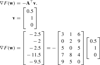
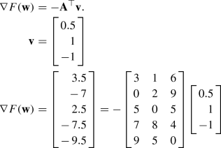
    $$\begin{aligned} \nabla F(\mathbf {w})= & {} -\mathbf {A}^\top \mathbf {v}.\\ \mathbf {v}= & {} \left[ \begin{array}{r} 0 \\ -\,1\\ -\,1\end{array} \right] \\ \nabla F(\mathbf {w})= & {} \left[ \begin{array}{r} 7 \\ 11\\ 5\\ 12\\ 5 \end{array} \right] = - \left[ \begin{array}{rrr} 3 &{} \quad 1 &{} \quad 6 \\ 0 &{} \quad 2 &{} \quad 9 \\ 5 &{} \quad 0 &{} \quad 5 \\ 7 &{} \quad 8 &{} \quad 4 \\ 9 &{} \quad 5 &{} \quad 0 \end{array} \right] \left[ \begin{array}{r} 0 \\ -\,1\\ -\,1\end{array} \right] \end{aligned}$$

    By taking the absolute value of the gradient

    $$\begin{aligned} |\nabla F(\mathbf {w})| = \left[ \begin{array}{rrrrr} 7&\quad 11&\quad 5&\quad 12&\quad 5 \end{array} \right] , \end{aligned}$$

    the following processing order of the weights is obtained:

    $$\begin{aligned} w_4, ~ w_2, ~ w_1, ~ w_5, ~ w_3 \end{aligned}$$

  • Iteration 3: processing the weights

    • Compute $F(\mathbf {w})$ by adjusting $w_4$ in the opposite direction of the gradient. For $w_4 - 1 = 4$: $F(\mathbf {w}) = 10.5$

      $$\begin{aligned} 10.5=(92-83)/(92-88-2)+(61-55)/(61-58-2) \end{aligned}$$

      Since if $w_4 = 4$, then $F(\mathbf {w}) > 5$, $w_4$ is not updated. Therefore, $w_2$ is consider next.

    • Compute $F(\mathbf {w})$ for $w_2 - 1=0$: Since $w_2$ cannot be 0, one cannot decrease $w_2$. Therefore, one moves to $w_1$.

    • Compute $F(\mathbf {w})$ for $w_1 - 1=5$: $F(\mathbf {w}) = 5.5$.

      $$\begin{aligned} 5.5= (92-87)/(92-88-2)+(72-69)/(72-69-2) \end{aligned}$$

      Since if $w_1 = 5$, then $F(\mathbf {w}) > 5$, it is not possible to update $w_1$. Therefore, one moves to $w_3$

    • Compute $F(\mathbf {w})$ for $w_3 - 1=1$: $F(\mathbf {w}) = 7.5$.

      $$\begin{aligned}&(92-85)/(92-88-2)+(61-63)/(61-64+2)\\&+\,(72-70)/(72-69-2)=7.5 \end{aligned}$$

      Since if $w_3 = 1$, then $F(\mathbf {w}) > 5$, there is no need to do update $w_3$. Therefore, one moves to $w_5$

    • Compute $F(\mathbf {w})$ for $w_5 - 1=2$: $F(\mathbf {w}) = 11.5$.

      $$\begin{aligned} 11.5= & {} (92-81)/(92-88-2)+(61-58)/(61-58-2)\\&\quad +\,(72-75)/(72-75+2) \end{aligned}$$

      Since if $w_5 = 2$, then $F(\mathbf {w}) > 5$, it is not necessary to update $w_5$. Therefore, the algorithm stops.

• Final Weights

  The final calibrated weights are

  $$\begin{aligned} \mathbf {w}^\top = \left[ \begin{array}{rrrrr} 6&\quad 1&\quad 2&\quad 5&\quad 3 \end{array} \right] . \end{aligned}$$

  The final calibrated totals are

  $$\begin{aligned} \hat{\mathbf {y}}= \left[ \begin{array}{rrr} 90&\quad 63&\quad 75 \end{array} \right] . \end{aligned}$$

By construction of the matrix $\mathbf {A}$, the summation of the weights is not part of the targets in this example. The purpose of this example is to show how the algorithm works rather than showing what type of results are attainable. At the end, the correlation between the initial vector of DSE weights and the final vector of calibrated weights is about 0.8, which is even higher than those obtained in the real case example provided in Sect. 3 (see Figs. 3 and 4).

References

Alho, J. M., Mulry, M. H., Wurdeman, K., and Kim, J. (1993). Estimating heterogeneity in the probabilities of enumeration for dual-system estimation. Journal of the American Statistical Association, 88(423):1130–1136.
Alho, J. M. (1990). Logistic regression in capture-recapture models. Biometrics, 46(3):623–635.
Antal, E. and Tillé, Y. (2011). A direct bootstrap method for complex sampling designs from a finite population. Journal of the American Statistical Association, 106(494):534–543.
Cauchy, A. (1847). Méthode générale pour la résolution des systemes déquations simultanées. Comp. Rend. Sci. Paris, 25(1847):536–538.
Cochran, W. G. (1978). Laplace’s ratio estimator. In Contributions to survey sampling and applied statistics, pages 3–10. Elsevier.
Deville, J.-C. (1988). Estimation linaire et redressement sur information auxiliaire d’enqutes par sondage.
Deville, J.-C. and Särndal, C.-E. (1992). Calibration estimators in survey sampling. Journal of the American Statistical Association, 87(418):376–382.
Duchesne, P. (1999). Robust calibration estimators. Survey Survey Methodology, 25:43–56.
Estevao, V. M. and Särndal, C.-E. (2000). A functional form approach to calibration. Journal of Official Statistics, 16(4):379–399.
Fetter, M. (2009). An overview of coverage adjustment for the 2007 census of agriculture. In Proceeding of the Government Statistics Section, JSM, pages 3228–3236.
Fetter, M., Gentle, J., and Perry, C. (2005). Calibration adjustment when not all the targets can be met. In Proceeding of the Survey Research Method section Statistics Section, ASA, pages 3031–3035.
Griffin, R. and Mule, T. (2008). Spurious Events in Dual System Estimation. Technical Report 2010-E-20, United States Department of Commerce, United States Census Bureau, Washington, DC.
Henry, K. and Valliant, R. (2012). Methods for adjusting survey weights when estimating a total. Proceedings of the 2012 Federal Committee on Statistical Methodologys Research Conference.
Hogan, H. (1993). The 1990 post-enumeration survey: Operations and results. Journal of the American Statistical Association, 88(423):1047–1060.
Horvitz, D. G. and Thompson, D. J. (1952). A generalization of sampling without replacement from a finite universe. Journal of the American Statistical Association, 47(260):663–685.
Kott, P. (2006). Using calibration weights to adjust for nonresponse and coverage errors. Survey Methodology, 32:133–142.
Kott, P. S. (2001). The delete-a-group jackknife. Journal of Official Statistics, 17(4):521.
Kott, P. S. (2004). Collected techincal notes on weighting and its impact to the 2002 census of agriculture. United States Department of Agriculture Report.
Lemel, Y. (1976). Une gnralisation de la mthode du quotient pour le redressement des enqutes par sondage. Annales de l’ins, (22/23):273–282.
Luo, Z. Q. and Tseng, P. (1992). On the convergence of the coordinate descent method for convex differentiable minimization. Journal of Optimization Theory and Applications, 72(1):7–35.
Mashreghi, Z., Haziza, D., Léger, C., et al. (2016). A survey of bootstrap methods in finite population sampling. Statistics Surveys, 10:1–52.
Mule, T. (2008). 2010 Census Coverage Measurement Estimation Methodology. Technical Report 2010-E-18, United States Department of Commerce, United States Census Bureau, Washington, DC.
Nutini, J., Schmidt, M., Laradji, I., Friedlander, M., and Koepke, H. (2015). Coordinate descent converges faster with the gauss-southwell rule than random selection. In Bach, F. and Blei, D., editors, Proceedings of the 32nd International Conference on Machine Learning, volume 37 of Proceedings of Machine Learning Research, pages 1632–1641, Lille, France. PMLR.
O’Donoghue, E., Hoppe, R. A., Banker, D., and Korb, P. (2009). Exploring alternative farm definitions: implications for agricultural statistics and program eligibility. Economic Information Bulletin-USDA Economic Research Service, 49.
Rao, J. and Singh, A. (1997). A ridge-shrinkage method for range-restricted weight calibration in survey sampling. In Proceedings of the section on survey research methods, pages 57–65. American Statistical Association Washington, DC.
Scholetzky, W. (2000). Evaluation of integer weighting for the 1997 Census of Agriculture. Technical Report RD-00-01, United States Department of Agriculture, National Agricultural Statistics Service, Washington, DC.
Singh, A. and Mohl, C. (1996). Understanding calibration estimators in survey sampling. Survey Methodology, 22(2):107–115.
Southwell, R. V. (1940). Relaxation Methods in Engineering Science—a Treatise On Approximate Computation. Oxford University Press, Oxford.
Théberge, A. (1999). Extension of calibration estimators in survey sampling. Journal of the American Statistical Association, 94(446):635–644.
Théberge, A. (2000). Calibration and restircted weights. Survey Methodology, 26(1):99–107.
Tibshirani, R. (1996). Regression shrinkage and selection via the lasso. Journal of the Royal Statistical Society. Series B (Methodological), 58(1):267–288.
Tilling, K. and Sterne, J. A. (1999). Capture-recapture models including covariate effects. American journal of epidemiology, 149(4):392–400.
Wright, S. J. (2015). Coordinate descent algorithms. Mathematical Programming, 151(1):3–34.
Xi, C. S. and Tang, C. Y. (2011). Properties of census dual system population size estimators. International Statistical Review, 79(3):336–361.
Young, L. J., Lamas, A. C., and Abreu, D. A. (2017). The 2012 Census of Agriculture: a capture–recapture analysis. Journal of Agricultural, Biological and Environmental Statistics, 22(4):523–539.
Young, L. J., Lamas, A. C., Abreu, D. A., Wang, S., and Adrian, D. (2013). Statistical methodology for the 2012 us census of agriculture. In the Proceeding 59th ISI World Statistics Congress, pages 1063–1068.
Author information
Authors and Affiliations
Corresponding author
Electronic supplementary material
Below is the link to the electronic supplementary material.