
Abstract
It is vital to optimize the drilling trajectory to reduce the possibility of drilling accidents and boosting the efficiency. Previously, the wellbore trajectory was optimized using the true measured depth and well profile energy as objective functions without considering uncertainty between the actual and planned trajectories. Without an effective management of the uncertainty associated with trajectory planning, the drilling process becomes more complex. Prior techniques have some drawbacks; for example, they could not find isolated minima and have a slow convergence rate when dealing with high-dimensional problems. Consequently, a novel approach termed the “Modified Multi-Objective Cellular Spotted Hyena Optimizer” is proposed to address the aforesaid concerns. Following that, a mechanism for eliminating outliers has been developed and implemented in the sorting process to minimize uncertainty. The proposed algorithm outperformed the standard methods like cellular spotted hyena optimizer, spotted hyena optimizer, and cellular grey wolf optimizer in terms of non-dominated solution distribution, search capability, isolated minima reduction, and pareto optimal front. Numerous statistical analyses were undertaken to determine the statistical significance of the algorithm. The proposed algorithm achieved the lowest inverted generational distance, spacing metric, and error ratio, while achieving the highest maximum spread. Finally, an adaptive neighbourhood mechanism has been presented, which outperformed fixed neighbourhood topologies such as L5, L9, C9, C13, C21, and C25. Afterwards, the technique for order preference by similarity to ideal solution and linear programming technique for multidimensional analysis of preference were used to provide the best pareto optimal solution.
Introduction
Present global oil and gas sectors are concerned about cost minimization and safety. The advantages of directional drilling have been known to the industry from its inception (Lu et al. 2014). Despite its high cost, this drilling allows the well path to be placed into productive intervals. With the growing use of directional drilling, it is vital to create solutions to all complex geological problems, necessitating optimization (Rahman et al. 2021b, c). Prior to drilling, optimizing the drilling trajectory decreases the chance of drilling accidents and boosts drilling efficiency. The literature demonstrates that most of the researcher focused on true measured depth (TMD), torque, well profile energy, rate of penetration as optimization objectives (Atashnezhad et al. 2014; Wood 2016; Abbas et al. 2018; Biswas et al. 2020b). It is also evident from the literature that by optimizing the aforementioned objectives, cost management and safety have been greatly enhanced. It is also worth noting that multi-objective optimization is far more effective than single-objective optimization when it comes to trajectory design (Biswas et al. 2021b). Researcher used cellular automata-based multi-objective hybrid grey wolf optimization and particle swarm optimization, multi-objective genetic algorithm, multi-objective cellular particle swarm optimization for optimizing the above-mentioned properties (Zheng et al. 2019; Biswas et al. 2020a, 2021a). Each of these parameters is optimized considering several tuning variables such as azimuth angle, dogleg severity, inclination angle, and kick-off point. However, these approaches have a number of disadvantages, including limited exploitation capabilities, trapping of local optima, non-uniform distribution of non-dominated solutions, and inability to follow isolated minima (Zheng et al. 2019).
However, another significant issue is the formulation of drill-string torque, which increases when TMD is reduced. Inadequate transmission of ground torque to the downhole has a detrimental influence on the safety and efficiency of drilling process (Huang et al. 2020). Additionally, the design of the wellbore has an effect on the torque delivered to the drill string (Sheppard et al. 1987). A significant dogleg angle or curvature, particularly for directional wells with a great depth of measure, results in a high drill-string torque (Mason and Chen 2007). This excessive amount of torque complicates the trajectory model. However, drill-string stress is basically affected either by bottom hole assembly (BHA), or by fluid. The friction and buoyancy factors can be used to calculate stress, which characterizes the relationship between drill-string torque and trajectory parameters (Hegde et al. 2015). Researchers developed different model to establish the aforesaid relationship. Several of them employed mechanical analysis to establish a correlation between torque and the trajectory’s geometric parameters, while others developed a discrete torque prediction model based on force measurements recorded at the drill string’s joint (Aadnoy et al. 2010; Fazaelizadeh 2013).
While optimization enables the simulation of a smooth planned trajectory, the actual trajectory may necessitate consideration of tortuosity. In drilling engineering, tortuosity refers to the volatile nature of a real-world drilling trajectory (Sugiura and Jones 2008). The varied inclination and azimuth angles along the trajectory reflect this event. If the trajectory plan's projection of drill-string torque proves to be wrong, the likelihood of an accident increases. When tortuosity is factored into the design of the drilling trajectory, it is possible to estimate the load on the drill string with more accuracy, which is beneficial (Samuel and Liu 2009; Boonsri 2014). Unlike TMD and torque, however, the total tortuosity of the trajectory cannot be computed simply summing the tortuosities of the trajectory's various sectors. Wendi Huang et al. demonstrated how to incorporate tortuosity into the computation of torque and demonstrated a multi-objective drilling trajectory optimization model to address the issue (Huang et al. 2018). Two objective functions were chosen for minimization in that work: TMD and the torque delivered to the modified drill-string during the drilling procedure. A sine function was used to describe tortuosity in that context, although this function can only approximate the situation approximately, not precisely (Samuel and Liu 2009). The probability density function of tortuosity can be estimated by conducting a statistical analysis on data that has been acquired from a real-world field. Uncertainty will be introduced into the optimization model as a result of the introduction of a parameter indicated by a probability density function (Ma et al. 2006). In this work, the problem of optimizing the drilling trajectory in the presence of parameter uncertainty is addressed, and as a result of this inquiry, a hybrid multi-objective optimization strategy with outlier removal mechanism is proposed.
This multi-objective problem (MOP) is a nonlinear and conflicting optimization problem. The multi-objective spotted hyena optimizer (MOSHO) is extremely effective at resolving this type of problem, as it has done previously (Dhiman and Kumar 2018; Panda and Majhi 2020; Biswas et al. 2021a; Naderipour et al. 2021; Şahman 2021). Apart from that, the previously employed NSGA II method for wellbore trajectory optimization has a number of disadvantages (OuYang et al. 2008; Zhu et al. 2016; Rahman et al. 2021a). However, SHO has an extremely high convergence rate (Ghafori and Gharehchopogh 2021). As a result, this technique ran into difficulties with local optima trapping during nonlinear optimization. To overcome this issue and the disadvantages of NSGA II, this work incorporates cellular automata (CA) with spotted hyena optimizer (SHO), which has a slow diffusion mechanism and the capability to exchange information with nearby neighbours. The CA mechanism stated previously assists in avoiding the problem of local optima trapping, and the information-exchanging capabilities aid in improving the algorithm's local search capability. Additionally, the particle swarm optimization (PSO) velocity update method has been integrated to enhance SHO's hunting capability, which is a new feature. The study makes the following significant contributions to the field:
-
1.
The torque prediction of the drill-string may be too optimistic if the difference between the actual and design trajectories is not taken into consideration, increasing the likelihood of an accident. Consequently, the tortuosity of the trajectory is incorporated to indicate the differences between the actual and design trajectories, and the difference is expressed as parameter uncertainties in multi-objective (MO) drilling trajectory optimization problem.
-
2.
A probability density function is formulated to predict the uncertainties in azimuth and inclination angle. This makes this problem a MOP with uncertainties.
-
3.
A modified multi-objective cellular spotted hyena optimizer (MOCSHO) is devised here, where CA is incorporated to overcome the shortcomings of SHO.
-
4.
An outlier elimination strategy is developed to deal with the abnormal data generated by uncertainty.
-
5.
An adaptive neighbourhood mechanism (AN) is proposed to address the shortcomings of fixed neighbourhood topological structures such as the L5, L9, C9, C13, C21, and C25.
Formulation of trajectory optimization problem
In order to solve the aforementioned problems of oil and gas industry and related uncertainties discussed in the above sections and to analyse the effect of uncertainties in these cases, they must first be formulated mathematically. Researchers have previously used a variety of methods to mathematically formulate the objective functions associated with trajectory optimization (Sawaryn and Thorogood 2003; Liu et al. 2004). This study's mathematical formulation is accomplished through the use of the radius of curvature method (RCM). The seven segments of the wellbore trajectory profile under consideration are depicted in Fig. 1.

Wellbore trajectory profile
In Fig. 1, TVD denotes the actual vertical depth of the entire trajectory, but the letters \({D}_{kop}\), \({D}_{D}\), and \({D}_{B}\) denote multiple vertical depths. However, each section’s length is marked by the letters \({D}_{1}-{D}_{5}\). Segment \({D}_{2}\) and segment \({D}_{4}\) represent the tangent and hold sections, respectively, with constant azimuth and inclination angles. Segments with variable azimuth and inclination angles, such as those found in segments \({D}_{1},{D}_{3},and {D}_{5,}\) are called build-up segments. According to method the constant of curvature \(a\), radius of curvature \(r\) and distance between two paths in a three-dimensional survey \(\Delta M\) can be formulated as follows
Here \({\theta }_{i}\), \({\mathrm{\varnothing }}_{i}\) represent the azimuth angle and inclination angle, respectively, and \(T\) stands for dogleg severity. segments. The following formulas (4–9) are derived to calculate the length of these segments.
Here \({r}_{1},{r}_{3}, {r}_{5}\) represent the curvature radius of segments \({D}_{1},{D}_{3},{D}_{5}\). Now the total length (TMD) can be formulated as Eq. (10).
When it comes to wellbore torque, it refers to the rate at which the osculating plane changes direction. That is, it reflects the binormal vector's rotation rate relative to the curved length. A complex trajectory structure implies large angle changes within segments, because curved and non-vertical sections have frequent angle fluctuations. Torque and drag evaluations, as well as optimization, are necessary to solve drilling issues.
When calculating the torque in this study, the soft string model is employed, in which the drill string is considered to be a soft rod (without rigidness) (Mirhaj et al. 2016). Depending on the segment type (straight or curved), the computation method changes. The axial weight is equivalent to the drag force in the straight segment of the trajectory. However, the contact between drill string and wellbore is responsible for the generation of torque. The following formulas are derived by using the analysis of force balance.
Here \({F}_{1}\) signifies the axial load applied to the bottom of the element, \({F}_{2}\) represents the axial load at the top of the element, while \(B\), \(w\), \(\Delta L\) stand for buoyancy factor and weight of unit pipe length, length interval, respectively. \(\mu\) and \(D\) stand for friction factor and pipe diameter, respectively. In this study, \(B=0.7\), \(w=0.3kN/ft\),\(\mu =0.2\) and \(D=0.2ft\). In case of curved section, azimuth and inclination angle changes often. To track these changes, data are collected from different survey point.
According to Fig. 2, \({P}_{1}\) and \({P}_{2}\) are two survey points, \({e}_{1},{e}_{2}\) denote two-unit vector whose direction is along the tangent of \({P}_{1}\) and \({P}_{2,}\) and \(\beta\) is the angle between them. Now according to the rule of scalar product.

Total change in direction \(\beta\) at points \({P}_{1}\) and \({P}_{2}\)
Now according to Fig. 3, Eq. (13) can be expressed as

Decomposition of vector \(e\) along different axis
After putting these equations into Eq. (14), it becomes
The overall directional change here is represented by \(\beta\). When the object's inclination and azimuth are both altered, the object's (\(\beta )\) acting plane is no longer limited to the horizontal or vertical plane. Then, by using the derivation from Biswas et al. (2021b) and Fazaelizadeh (2013) the axial force and torque can be calculated as follows
Now to calculate the total torque, the axial loading of each part can be calculated as follows:
Torque of each segment is as follows
After calculating the torque of each segment, the total torque can be expressed as follows:
When predicting the torque, the accuracy of torque prediction is greatly influenced by the tortuosity of the actual drilling trajectory. Tortuosity is defined in this work in terms of the chganges in azimuth and inclination angles along a given length of the trajectory segment. The probability density function is as follows, according to Fu (2013).
Here \(x=\) \({\mu }_{\varnothing },{\mu }_{\theta }\) represent the change rate of inclination angle, azimuth angle ( ̊/m) which are both regulated by Gaussian distributions. Values of constant A, B can be determined through statistical procedure. Variations in angles introduces uncertainty into the torque computation. After the adjustments, the inclination and azimuth angles are as follows:
Operational and inequality constraints
The proposed strategy is evaluated in this work using real-world data from the Gulf of Suez (Shokir et al. 2004; Biswas et al. 2021b). The trajectory under investigation has some operational constraints, non-negative constraints and inequality constraints. TVD and casing setting depth (\({C}_{i})\) are example of operational constraints which are formulated in Eqs. (27–31). However, the proposed algorithm needs to optimize 17 tuning variables in this research which are tabulated in Appendix A Table A1 and their constraint limit in Table A2. Besides, TMD and torque are expressed as non-negative constraints.
where \({Y}_{1}\) represents the vertical depth of \({D}_{kop}\) section and \({Y}_{2}-{Y}_{6}\) denote the vertical depth of \({D}_{1}-{D}_{5}\).
For smooth operation, it is necessary to keep the trajectory within the target. For that, the spatial position of the end point should be controlled. The coordinate of the \({i}_{th}\) point on the trajectory can be devised as
where the value of dogleg angle \({\beta }_{i}\) value can be found from Eq. (18). \({N}_{i}\), \({E}_{i}\), represent the coordinate of point \(i\) at north and east direction, and \({D}_{i}\) represent the vertical depth. However, the coordinate of the straight section can be obtained by using the following equations.
Framework for hybrid optimization approach
As part of this multi-objective optimization process, the proposed hybrid algorithm must optimize the length (TMD) and torque, based on Eqs. (10), (22).The algorithm have to fine-tune all 17 tuning variables simultaneously in order to optimize these objectives. The followings are the mathematical representation of the overall multi-objective optimization process.
However, after incorporating probability density function of tortuosity, torque’s expected value can be expressed as
But the equation signifies that during each iteration of optimization the algorithm needs to calculate \({T}_{\mathrm{ex}}\) for every single \(x,\) which will significantly influence the computational time. That’s why random sampling is used to calculate the \({T}_{\mathrm{ex}}\). According to Wiener–Khinchin law of large numbers, when M is big enough the expected value can be estimated by
Here \(x and {\mu }_{m}=({\mu }_{\O ,m},{\mu }_{\theta ,m})\) denote the decision parameter and uncertain parameter, respectively. However, the probability function of \({\mu }_{\O },{\mu }_{\theta }\) can be represented by \(P\left({\mu }_{\O }\right),and P\left({\mu }_{\theta }\right),\) respectively. Prior to optimizing these objective functions, it is critical to identify outliers that could distort the process. In this work, usually torque is affected by the random parameter which is also can be denoted as an outlier. Therefore, an outlier elimination strategy was devised for a smooth optimization process. According to the criterion, any data that are more than three standard deviations away from the mean value are considered an outlier. This study assigned the largest nondomination rank to identified outliers.
In this work, modified MOCSHO with outlier elimination mechanism was applied to optimize the objective functions, since it has the capability to handle the non-linearity and constrained of MO problem. The proposed method employed the diffusion mechanism of CA to enhance the exploration capabilities of SHO, and it afterwards used the velocity update equation of PSO to update the velocity of the SHO. SHO’s hunting mechanism was improved as a result of this.
Spotted hyena optimizer
The metaheuristic algorithm has been devised in response to the hyena’s prey hunting mechanism and it is outlined below (Dhiman and Kumar 2018). The SHO algorithm simulates a hyena cluster's behaviour. It is subdivided into four stages: searching, encircling, hunting, and attacking. The first stage is the “searching”. During this phase, a group of peers guides the hunter towards the ideal solution while preserving optimal results. The equations below simulate the spotted hyenas' circling interactions.
where \(\overrightarrow{{M}_{h}}\) denotes the distance between the prey and the spotted hyena, \(x\) is the current iteration, \(\overrightarrow{A}\) and \(\overrightarrow{F}\) denote the coefficient vectors, \(\overrightarrow{{Q}_{p}}\) denotes the position vector of the prey, and \(\overrightarrow{Q}\) denotes the position vector of the spotted hyena. Aside from that, the characters || and “.” signify the absolute value and vector multiplication, respectively. In order to determine the vectors \(\overrightarrow{A}\) and \(\overrightarrow{F}\), the following formulas are utilized:
where Iteration equals 1, 2, 3,…. \({\mathrm{Max}}_{\mathrm{Iteration}}\). The vectors r \(\overrightarrow{{d}_{1}}\) and r \(\overrightarrow{{d}_{2}}\) in the range [0,1] are generated at random. The search agent is able to explore different parts of the search space by adjusting the values of the vectors \(\overrightarrow{A}\) and \(\overrightarrow{F}\). An adaptable hyena can change its location in relation to its prey by using Eqs. (48–50). This algorithm ensures that the best solutions remain in place and that others are compelled to improve their positions as a result. The algorithm authorizes the hyenas to attack their victim when \(|\overrightarrow{F|}\)<1 is reached. For imitating hyena hunting behaviour and identifying areas of prospective search space, it is necessary to develop the following equations.
Similarly, where (\(\overrightarrow{{Q}_{h}}\)) indicates the location of the first best-spotted hyena, (\(\overrightarrow{{Q}_{k}}\)) indicates the position of other search agents. In the case of spotted hyenas, the number N is represented by the following equation:
where \(\overrightarrow{G}\) is a random vector in the range [0.5,1], and nos specifies the number of solutions obtained after \(\overrightarrow{G}\) has been included. Furthermore, \(\overrightarrow{{D}_{h}}\) is a collection of optimal solutions with an N-number of possibilities.
Exploitation
During the course of exploitation, the value of \(\overrightarrow{h}\) drops steadily from 5 to 0. Additionally, the variance in \(\overrightarrow{F}\) has an impact on exploitation. When the prey becomes |< \(\overrightarrow{F|}\)1, the algorithm allows the hyenas to attack it because of the algorithm. The following is an expression for the formulation:
where \(\overrightarrow{Q}\left(x+1\right)\) keeps track of the optimal position and assists the search agent in adjusting their position in line with the optimal search agent.
Exploration
At the time of exploration, the primary responsible hyenas are of the vector \(\overrightarrow{{D}_{h}}\). When the exploration is performed, \(\overrightarrow{F}\) becomes either |> \(\overrightarrow{F|}\)1 or |< \(\overrightarrow{F|}\)-1. It generally exercises control over the hyenas in order to conduct global searches. The value of \(\overrightarrow{F}\) compels agents to diverge from optimal solutions, hence broadening the range of exploration and avoiding local optima. Another significant component is the vector \(\overrightarrow{A}\), which offers random values in the range [0.5,1] to the prey. In order to improve their positions during optimization, search agents apply Eqs. (53–55) to form a cluster towards the best search agent. Meanwhile, as iterations progress, the parameters h and \(\overrightarrow{F}\) decrease linearly. Finally, once the termination condition is satisfied, the positions of search agents composing a cluster are regarded optimal. The detail description of multi-objective spotted hyena optimizer (MOSHO) is given by Dhiman and Kumar (2018).
Cellular automata
Von Neumann and Ulam first introduced the concept of CA (Neumann and Burks 1966; Maignan and Yunes 2013). It is a distribution of cells created within a particular topological structure. Each cell's future state will be determined by the current states of all its neighbouring cells and so on. CA is made up of several components: the cell, the cell state, the cell space, the neighbourhood, and the transition rule, etc. Cell state is defined as the data contained within the currently selected cell. It contributes to the evaluation of the subsequent state. In a matrix, cell space is used to represent a collection of cell sets. It has a wide range of applications (one, two, and three). Due to the fact that real-world processes are generally represented by finite grids, it is vital to identify the cell space's boundary during the operation. A ring grid defines this boundary. Thus, the left border will remain connected to the right border, as well as the top border to the bottom border. The neighbourhood can be thought of as a collection of cells that are next to a central cell and so regarded to be its neighbours. Its primary purpose is to determine the next state to be picked. The transition rule determines the future state of the cell based on the state of neighbouring cells. The formulation of CA can exhibit the following features. The most frequently used metaphor for an m-dimensional CA is that it is a grid of m-dimensional single cells. Each cell holds a single value that cannot be duplicated. In accordance with the transition rule, each cell has the ability to update its state. As a result, the mathematical formulation of cellular automaton Q may be expressed as follows
where.The finite set of state: T, Dimension of Q: d ∈ Z + Neighbourhood: H, Transition rule: g
Let’s take i ∈ \({Z}^{m}\) is the position of a cell where m is the dimension of the lattice grid, then the neighbourhood H can be formulated as
where neighbourhood size is represented by n; a fixed vector from the search space of m-dimension is represented by \({r}_{j}\).
Neighbourhood
Neighbours are a collection of cells that surround a central cell in a ring-like formation. In addition, the neighbours can be defined as the other atoms that are related to a single atom by a single bond. The neighbours of the grid are defined in this work depending on their direction and radius. There are two structural labels that are commonly used to refer to it. They are denoted by the letters \({L}_{n}\) and \({C}_{n}\). If there are n—1 nearest neighbours in the direction of the centre cell, the structure is denoted by the letters \({L}_{n}\) or \({C}_{n}\), respectively.
If the directions of neighbouring cells are at the top, bottom, left, and right, then it will be denoted by \({L}_{n}\). Alternatively, when the directions are at the top, bottom, left, right, and diagonal, it will be symbolized by \({C}_{n}\). In this research, six types of classical structure have been used to analyse the impact of neighbourhood structure. These structures are L5, L9, C9, C13, C21, and C25 which are depicted in Fig. 4.

Different types of neighbourhood structure
Transition rule
To handle the issue of each atom transitioning from one state to the next, the transition rule is applied. This rule establishes the transformation process by employing data from the neighbouring cells. The neighbour with the highest fitness value among the neighbours will be used to facilitate information diffusion. If \({M}_{i}\) denotes the optimal neighbour and \({P}_{i}^{t}({M}_{n})\) denotes its location, the transition rule can be defined as follows.
where \(\mathrm{fitness }\left({P}_{i}^{t}\left({M}_{i}\right)\right)\) denotes the current value of \({M}_{i}\). Thus, the best optimal neighbour can be determined from the neighbourhood with the help of Eq. (58). Then, the elected one will be used to update the present state of the current cell.
Particle swarm optimization
This algorithm is a stochastic, population-based evolutionary technique that is inspired by the flocking behaviour of birds (Kennedy and Eberhart 1995). It is composed of two distinct processes. Both of these processes are carried out by birds. To begin, the bird will do a random search for the nearest region of food. Later on, it will use its flying experience to locate the food. The candidate solution is represented in the process by a bird, which is referred to as a particle. Additionally, food serves as a representation of the optimal solution. The position of a particle varies as a result of particle interaction, and the rate of position change is referred to as velocity. Throughout the flight, the particle's velocity varied randomly in the direction of its finest point (personal best) and in the direction of the community's best solution (global best). In conclusion, the knowledge and experience of swarm’s neighbours have an impact on the evolution of each particle.
In this work, \({X}_{i}={X}_{i1}, {X}_{i2}, {X}_{i3}\dots .{X}_{id}\), represents the \({i}^{th}\) particles, whereas velocity is represented by \({v}_{i}={v}_{i1}, {v}_{i2}, {v}_{i3}\dots .{v}_{id}\). According to the mechanism, each particle initiates the random searching in the search space with their initial velocity, where \({p}_{i}={p}_{i1}, {p}_{i2}, {p}_{i3}\dots .{p}_{id}\) represent the particle's personal best position, whereas \({p}_{g}={p}_{g1}, {p}_{g2}, {p}_{g3}\dots .{p}_{gd}\) represent the global best position of each particle. PSO updates the velocity and position of each particle using the following equations.
Here acceleration coefficients are \({c}_{1}\) and \({c}_{2}\) that primarily controls algorithm’s exploration and exploitation capability, inertia weight is denoted by \(w\), whereas \({r}_{1}and {r}_{2}\), are random numbers between [0,1]. The fitness value is used to determine the best particle's quality. The particle with the highest fitness value is considered to be the global best one (Coello et al. 2004).
Hybridization
In order to address the issues experienced by the SHO, this research made use of the CA's neighbourhood formation mechanism for trajectory optimization. PSO, on the other hand, is employed to improve the hunting mechanism of SHO. The following three advantages motivate the improvement strategy.
-
Due to the fact that CA enhances exploitation capability through interaction with its neighbours, CA can be employed to enhance SHO's local search capabilities. On the other hand, information transfer facilitates the exploration process.
-
Because the resultant solutions of the candidates are attracted towards the good SHO solutions, the convergence speed of the SHO is relatively fast, resulting in a trapping of local optima in the process of convergence. The slow diffusion mechanism of CA in conjunction with SHO will aid the SHO in avoiding the local optima trap.
-
The SHO's hunting mechanism will be enhanced by using the PSO's velocity update technique. Typically, the velocity component of PSO is regulated by multiplying the particle's velocity by a constant factor. The purpose of this velocity management is to achieve a balance between exploration and exploitation.
This programme generates populations of spotted hyenas that are semi-randomly distributed. It consists of n-dimensional lattice grids that are randomly distributed. In the approach that has been proposed, the operational constraints are managed during the initialization of the agent's positions. Once this is done, the tuning variables for the wellbore trajectory \({x}_{j}\) are initialized at random but in a limited environment in order to get the desired outcomes. If the starting positions satisfy the operational and non-negative requirements, they are accepted without further consideration. Otherwise, they are rejected. As a result of this strategy, the values of the initial tuning variable will be less chaotic. The fitness value of each population is then computed in terms of wellbore trajectory optimization. This is followed by the start of the update loop. It makes use of the CA principle in order to establish a new neighbourhood. During the process of creating a neighbourhood, some of the neighbours will overlap. It permits the algorithm to include an implicit migration mechanism. Additionally, it contributes to the seamless diffusion of the most effective solutions throughout the population. A larger degree of diversity than the original SHO can be maintained as a result of this transformation. Soft diffusion is essential for maintaining a healthy balance between exploration and exploitation of natural resources. This strategy divides the total search area into multiple sub-search regions, each of which is a separate search space. As a result, they will be able to update the operation independently. However, if the neighbours overlap in this case, information is transferred on an ad hoc basis rather than in a systematic manner.
The hunting mechanism of SHO, on the other hand, has been updated by including the velocity update method of PSO (Dhiman and Kaur 2019). As a result, the following is an expression for Eq. (61).
The proposed algorithm will make use of the newly revised hunting mechanism to accomplish its goals. The following is the pseudocode for the algorithm that has been proposed:

Adaptive neighbourhood
Each search agent will construct a neighbourhood based on its fitness value, according to the proposed method. If the search agent is of superior value, the result will be the establishment of a sizable neighbourhood. It will improve the likelihood of intersecting with the most effective one. Additionally, it will increase the diversity of the solutions, which will aid in avoiding the local optima trap and other issues. The BL approach is a type of strategy that is used in this situation (Dorronsoro and Bouvry 2013). In the case of the BS approach, on the other hand, the worst search agent will construct a big, sizable neighbourhood in order to maximize the odds of interacting with the better agents (Dorronsoro and Bouvry 2013). As a result, the quality of suboptimal solutions will increase. Thus, the algorithm will benefit from two strategies: avoiding the local optima trap or refining suboptimal solutions. Apart from that, both will retain their uniqueness. Each search agent's neighbourhood will be created by the algorithm in accordance with the following methodology when the algorithm attempts to establish a neighbourhood for each search agent.

Wellbore trajectory optimization mechanism
For optimization, 500 search agents were taken and iteration number was selected as 100 in this work. Later the statistical method of Fu (2013) was utilized to fit the probability density function of \({\mu }_{\emptyset } \ and \ {\mu }_{\theta }\).
The concern now is what the value of M (Eq. 45) will be. M is determined by setting \(x\) is to its upper limit and then computing \({T}_{ex.}\) The objective was to find the value of M, for which it will give relatively small error, that is, less than 0.1%. Finally, the value of M = 1000 was used in this work, which resulted in a relative error of 0.29%. It was an acceptable value that will have little effect on the optimization process. Following that, an outlier removal mechanism was applied to handle the abnormal data. Later in the approach, the spotted hyena populations were initialized semi-randomly to make the approach less chaotic. After evaluating each search agent, it selected the best search agents and clusters of all obtained solutions for the wellbore trajectory optimization problem. A neighbourhood then designed using an adaptable neighbourhood (AN) topology because of this. Additionally, this scenario evaluated both the fixed structure (L5, L9, C9, C13, C21, C25) and the AN structure. After they had been built using the CA technique, they were analysed for optimization issues as well as constraint violation. Afterwards, they shared their newfound knowledge with one another. The most optimal solution was provided by any neighbour who was able to deliver a solution that was superior to the current agent's solution (central cell). In all other cases, the central cell was the most optimal. It was then repeated till the end criterion was met.
Result and discussion
In this subsection, the performance of proposed algorithm for well bore trajectory optimization will be analysed. For comparison several state-of-the-art algorithms, multi-objective cellular spotted hyena and particle swarm optimization (MOCSHOPSO) without outlier removal mechanism, multi-objective spotted hyena optimizer (MOSHO), multi-objective cellular grey wolf optimization (MOCGWO) were selected (Dhiman and Kumar 2018; Lu et al. 2018). During comparison, the stopping criteria were maximum number of iterations. For qualitative and quantitative analysis, inverted generational distance (IGD), maximum spread (MS), spacing metric (SP), error ratio (ER) were selected as comparative criterion. Moreover, a spearman corelation coefficient analysis test was performed to sort out the most prominent parameter during optimization.
Outcome of proposed algorithm
True measured depth and torque were mathematically modelled for this wellbore trajectory optimization. To substantiate the performance and effectiveness of the proposed algorithm, these objective functions were utilized as wellbore trajectory optimization problem. Results of interest are demonstrated in bold expression in the relevant tables to highlight the capabilities of the proposed algorithm.
All results were obtained based on the overall out-comes of 30 randomly initialized independent runs and during 100 internal iterations to evolve 500 search agents in each algorithm. All results obtained in this research were recorded using a single computer, and all tests were carried out in a same condition to have a fair comparison. To investigate the efficacy of the proposed algorithm in solving this problem, it was compared to several state-of-the-art methods. Figure 5 depicts the pareto front obtained by different algorithms. According to Fig. 5, it is visible that the torque decreases as the length increases. Here the proposed method with outlier removal mechanism has shown better performance than others. Since it is important to control uncertainty than cost minimization, the Monte Carlo (MC) method had been applied here to illustrate the uncertainty and reliability of these pareto solutions (Luo et al. 2014).

Pareto optimal solutions obtained by different algorithm
This method finds out the upper and lower bound of the objective functions. For MC analysis, root mean square error (RMSE) and bandwidth were utilized according to the following equations
where the run time of optimization process is denoted by \(N\), \({F}_{i}= {[f}_{\mathrm{2,1},}{f}_{\mathrm{2,2}},\dots {f}_{2}, {N}_{p}]\) is the \({f}_{2}\) value of all individuals in pareto solutions obtained by the \({i}_{th}\) trial. \({F}_{u,i}\) and \({F}_{l,i}\) are the upper bound and lower bound of \({F}_{i}\), respectively. \({F}_{Avg}\) is the average value of \({F}_{i}\) among \(N\) times trial.
Each optimization algorithm was run for 30 times to statistically obtain the average value of RMSE and bandwidth. All the obtained results are tabulated in Table 1. From the recorded data in Table 1, it is visible that proposed method has the lowest RMSE value (20.234) and bandwidth (132.401) among the compared algorithms. On the other hand, MOCSHOPSO which is also an improved version of MOSHO has obtained the second smallest value (22.043) for both RMSE and bandwidth. It means that solution provided by the proposed method is superior and most reliable among the compared algorithms. Proposed method with outlier mechanism has achieved lower RMSE value than the MOCSHOPSO. It indicates that outlier removal mechanism is effective in minimizing uncertainties.
For allowing the decision maker to take final pareto solutions, the pareto solutions with smallest bandwidth obtained by the compared algorithms are tabulated in Table 2. It is found that the obtained solutions by the proposed method have achieve the smallest bandwidth. This clearly implicates that within uncertainty the obtained solutions by the proposed method have achieved better stability. Data from Table 2 also indicate that the proposed method has successfully obtained the smaller length and torque, which is clearly in line with the proposed goal.
In this work, TOPSIS and LINMAP analysis were also done to provide the decision maker the best pareto solutions (Ahmed et al. 2021). But it slightly defers from the solutions provided according to smallest bandwidth. The solutions are provided in Table 3.
Qualitative analysis
To demonstrate the efficacy and qualitative performance of the proposed algorithm, the obtained results are statistically analysed by performing several well-known statistical tests. In this subsection, the description and analysis of this statistical test will be discussed.
-
A.
Inverted generational distance (IGD)
From the above solutions, a researcher can develop two different kinds of pareto solutions. The pareto front solution and the approximation pareto front solution are two different sorts of solutions. The IGD illustrates the difference between these two. However, in order to calculate IGD, a true pareto front must be used. When the true pareto front is not available, non-dominated solutions serve as a point of reference. The formulation of IGD can be derived as
$${\text{IGD}}\left( {Q,Q^{*} } \right) = \frac{{\mathop \sum \nolimits_{i = 1}^{\left| Q \right|} d\left( {Q,Q^{*} } \right)}}{\left| Q \right|}$$(66)\(d\left(Q,{Q}^{*}\right)\) is the difference in Euclidean distance between the true pareto front (\(Q\)) and the approximation pareto front (\({Q}^{*}\)). If an algorithm obtains the lowest IGD value among comparable algorithms, it has obtained a pareto front that is very close to the true pareto front.
-
B.
Spacing metric (SP)
If the beginning and ending points of a pareto front are not known, it is necessary to calculate the distribution of solutions. SP is a metric that quantifies the distance variance between adjacent vectors in the resulting non-dominated solutions. The smallest value of SP implies that the solutions are quite close to one another in proximity. It expresses those solutions that are not dominated have a more even distribution than solutions that are dominated in some way. The following is the metric to use.
$${\text{SP}} = \sqrt {\frac{1}{{\left| {P - 1} \right|}}\mathop \sum \limits_{i = 1}^{\left| P \right|} \left( {d_{i} - \overline{d}} \right)^{2} }$$(67)where\({d}_{i}={min}_{j}(\left|{f}_{1}^{i}(\overrightarrow{x})-{f}_{1}^{j}(\overrightarrow{x})\right|+\left|{f}_{2}^{i}(\overrightarrow{x})-{f}_{2}^{j}(\overrightarrow{x})\right|)\), \(i,j=\mathrm{1,2},\dots n\), the average value of all \({d}_{i}\) is represented by\(\overline{d }\), and the total number of obtained pareto solutions is represented by \(P\)
-
C.
Maximum spread (MS)
This indicator is commonly used to calculate the diversity of the solutions that have been obtained as well as the covering area of the solutions. It is generally modelled as a difference between the two boundary solutions in a given situation.
$$MS = \sqrt {\mathop \sum \limits_{i = 1}^{0} {\text{max}}\left( {d\left( {a_{i} ,b_{i} } \right)} \right)}$$(68)Here the maximum values in \({i}^{\mathrm{th}}\) the objective is represented by \({a}_{i}\) and minimum values are represented by \({b}_{i}\).
-
D.
Error ratio (ER)
This metric quantifies the number of solutions that do not have a guaranteed spot in the resulting pareto optimal set. It can be expressed mathematically as follows.
$${\text{ER}} = \frac{{\mathop \sum \nolimits_{i = 1}^{n} e_{i} }}{n}$$(69)where the number of vectors in the currently available nondominated set is represented by \(n\), \({e}_{i}=0\mathrm{ if i\epsilon pareto optimal set}\) otherwise \({e}_{i}=1\). But ER = 0 is an ideal case that does not mean all solutions obtained by the proposed algorithm are within pareto optimal set.
During the qualitative and statistical analysis, each of the comparative algorithm was run 30 times in MATLAB software and all the results of interest for IGD, MS, SP and ER are tabulated in the respective tables. Based on the collected output, box plots are generated for the above-mentioned analysis because the box plot demonstrates the distribution, dispersion, and symmetry of solutions more precisely than any other plot. After performing the IGD analysis test, the recorded data are tabulated in Table 4 and the corresponding box plot is illustrated in Fig. 6.
Table 4 Output of comparative IGD analysis Fig. 6 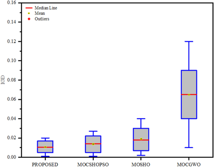
Box plot for IGD metric
From the recorded data in Table 4, it appears that the proposed algorithm has obtained a mean value of 0.0106 which is the lowest among the compared algorithms. However, the best value obtained by the proposed algorithm is 0. 0051. The second-best mean value was achieved by MOCSHOPSO without outlier removal mechanism which is also a hybrid version of MOSHO with the incorporation of CA. Since IGD justifies the performance of an algorithm by simultaneously evaluating its convergence and diversity, an obtained lowest IGD mean value by the proposed algorithm means it has a better convergence and diversity than other algorithm. Moreover, it also means that the obtained pareto front is nearer to the true pareto front.
After performing MS and SP statistical analysis in the same manner, their analysed data are tabulated in Tables 5 and 6, respectively, and the data are compiled in the form of box plot in Figs. 7 and 8, respectively. The data recorded in Table 5 have expressed that the proposed algorithm has the highest mean value (86.5281) in the case of MS statistical analysis, which means that the diversity of the solutions obtained by the proposed algorithm is highest. However, the standard deviation obtained by the proposed algorithm is 5.0146, the lowest among the comparative algorithms. CA diffusion mechanism assisted the search agent to diversify the solutions.
Table 5 Output of comparative maximum spread analysis Table 6 Output of comparative spacing metric analysis Fig. 7 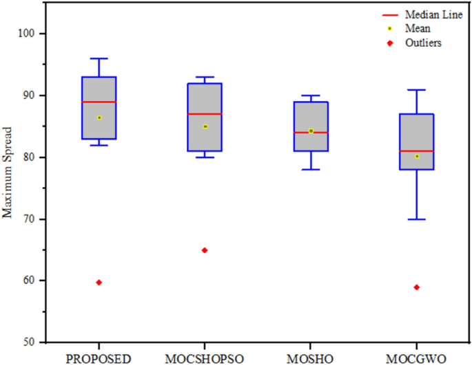
Box plot for maximum spread
Fig. 8 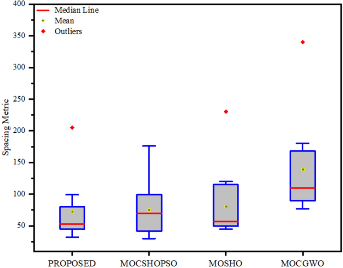
Box plot for spacing metric
Similarly, the data of SP analysis mentioned in Table 6 show that the mean value of the proposed algorithm is the lowest (72.5432) among the comparative algorithms, but in this case MOSHO has achieved the lowest standard deviation of 29.0963. Overall, the standard deviation is too high for all the algorithms.
The ER statistical test was subsequently performed to qualitatively analyse the performance of the proposed algorithm, the value of which is recorded in Table 7 and illustrated in the form of box plot in Fig. 9. Table 7 shows that the ER of the proposed algorithm has the lowest mean value among the compared algorithms and the lowest among all in the case of standard deviation. The mean value for the proposed algorithm is 0.1143, and the standard deviation is 0.0401 which is almost near to zero.
Table 7 Output of comparative error ratio analysis Fig. 9 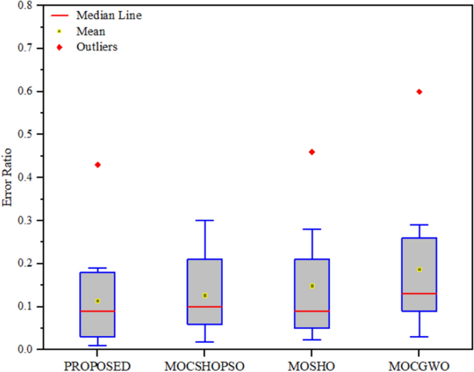
Box plot for error ratio


Performance analysis with different neighbourhood
Cellular automata can be used to construct different types of topologies, each of which performances is differ in term of quality. The algorithm proposed in this study is subject to six different conventional neighbourhood topologies and compared with the proposed adaptive neighbourhood topology for comparison purpose. IGD statistical test had been performed to qualitatively compare those mentioned topologies, and recorded data are tabulated in Table 8. These data are depicted in the form of box plot in Fig. 10. From the tabulated data in Table 8, it is clearly visible that the proposed algorithm has given best performance with C21 neighbourhood structure among the conventional topologies, but in terms of performance the proposed AN topology has surpassed that of C21. Table 8 shows that AN has a mean value of 0.3691 which is less than C21’s mean value of 0.5308 and even in the case of standard deviation the value of AN is lowest which is 0.0121. These improvements justify the incorporation of BL and BS strategy. The Friedman test was also used for multiple comparison which is the most common no parametric analysis. The data of this test are tabulated in Table 9 which shows that the p value of this test is 0.0537 and the rank value of AN in the test is 2.4503 which is slightly better than C21.

IGD comparison metric for neighbourhood comparison
One of the specific properties of constructed neighbourhood is their radius, based on which the algorithm decides whether to give more importance on exploration or to exploitation. However, the best results are given by a neighbourhood that balances the two and maintains convergence speed, misses a smaller number of significant optimal solutions, and avoids local optima trap. In order to test which radius of adaptive neighbourhood can best balance these two properties, its IGD analysis had been tested according to different radii which are tabulated in Table 10. Table 10 shows that the best performance is given by R = 1.5 with mean value of 0.2278 and variance 0.0179 which is lowest among all. This is also justified by Fig. 11 where the data have been presented as a box plot.

IGD comparison metric for different radii
Sensitivity analysis
The outputs in this study are dependent on 17 independent variables, each with its constraint limit. Sensitivity analysis is needed to find out how different values of these 17 independent variables affect the output based on a given assumption. Sensitivity analysis is of two types, out of which local sensitivity analysis expresses the relevance of each variable but does not reveal any correlation information in the case of multi-objective optimization. However, with the global sensitivity analysis, adjustment of any variable, a correlation between all the objectives is recognized. Due to the nonlinear nature of wellbore trajectory optimization, global sensitivity analysis was performed in this case. There are several statistical measure to find out the correlations; among them, Spearman correlation coefficient test is selected because it is very useful for non-normally distributed continuous data and is relatively robust for outliers. Spearman rank correlation is a measure of statistical dependence between two variables that is able to better account for non-linear relationships compared to conventional Pearson Correlations (Myers and Sirois 2004). The values can range from -1 to 1, with 0 indicating that there is no relationship. A Spearman rank correlation of 1 indicates a perfect, monotonically increasing relationship, while − 1 indicates a perfect, monotonically decreasing relationship. Therefore, the higher the absolute value of this number, the more important the reaction is. After performing the statistical test, the data observed are recorded in Table 11. The values of the three most significant variables for each objective are highlighted in the table.
Conclusion
Operational cost and risks are major concerns for the oil and gas industry worldwide. In this context, the industry needs a strategy that addresses the aforementioned issues and uncertainties involved in the design of real-world trajectory design problem. Meanwhile, a real-world trajectory was mathematically modelled using a probability density function to account for uncertainty. In this scenario, this work established a model termed the “modified MOCSHO”, which enables the operator to fix the optimal parameter with the least amount of uncertainty possible during trajectory design. The original SHO algorithm was improved during hybridization by adapting the slow diffusion mechanism of CA and the velocity update mechanism of PSO. These two approaches contributed significantly to overcoming the SHO's drawbacks, as demonstrated by the proposed algorithm's performance during trajectory optimization and improved performance during IGD, MS, SP, and ER analysis. The algorithm achieved lowest value of IGD (0.0106), SP (72.5432), ER (0.1143) and highest value of MS (86.5281) among the compared algorithm during performance evaluation. Thus, it can be concluded that the CA's slow diffusion mechanism aided the SHO in enhancing its exploration capability and avoiding local optima trapping. On the other hand, PSO's velocity update mechanism aided in the enhancement of the hunting mechanism and the maintenance of a more balanced approach to exploration and exploitation. Because the algorithm had to deal with abnormal data in real-world applications, it was updated with an outlier removal mechanism that contributed in reducing uncertainty during trajectory optimization. This research established that the hybrid algorithm version with an outlier removal mechanism outperforms the one without an outlier removal mechanism, as demonstrated by MC analysis. To overcome the disadvantages of fixed neighbourhood topologies (L5, L9, C9, C13, C21, and C25), AN is developed, and IGD analysis demonstrates its superiority. Additionally, this research established that R = 1.5 can improve the performance of AN.
References
Aadnoy BS, Fazaelizadeh M, Hareland G (2010) A 3D analytical model for wellbore friction. J Can Pet Technol 49:25–36
Abbas AK, Alameedy U, Alsaba M, Rushdi S (2018) Wellbore trajectory optimization using rate of penetration and wellbore stability analysis. In: SPE international heavy oil conference and exhibition. OnePetro
Ahmed R, Mahadzir S, Rozali NEM et al (2021) Artificial intelligence techniques in refrigeration system modelling and optimization: a multi-disciplinary review. Sustain Energy Technol Assess 47:101488
Atashnezhad A, Wood DA, Fereidounpour A, Khosravanian R (2014) Designing and optimizing deviated wellbore trajectories using novel particle swarm algorithms. J Nat Gas Sci Eng 21:1184–1204. https://doi.org/10.1016/j.jngse.2014.05.029
Biswas K, Islam T, Joy JS, Vasant P, Vintaned JAG, Watada J (2020a) Multi-objective spotted hyena optimizer for 3D well path optimization. Solid State Technol 63(3). https://www.researchgate.net/publication/345740975_Multi-Objective_Spotted_Hyena_Optimizer_for_3D_Well_Path_Optimization
Biswas K, Vasant PM, Vintaned JAG, Watada J (2020b) A review of metaheuristic algorithms for optimizing 3D well-path designs. Arch Comput Methods Eng 28:1775–1793
Biswas K, Rahman MT, Negash BM et al (2021a) Spotted hyena optimizer for well-profile energy optimization. In: Journal of physics: conference series. IOP Publishing, p 12061
Biswas K, Vasant PM, Vintaned JAG, Watada J (2021b) Cellular automata-based multi-objective hybrid Grey Wolf Optimization and particle swarm optimization algorithm for wellbore trajectory optimization. J Nat Gas Sci Eng 85:103695
Boonsri K (2014) Torque simulation in the well planning process. In: IADC/SPE Asia pacific drilling technology conference. OnePetro
Coello CAC, Pulido GT, Lechuga MS (2004) Handling multiple objectives with particle swarm optimization. IEEE Trans Evol Comput 8:256–279
Dhiman G, Kaur A (2019) A hybrid algorithm based on particle swarm and spotted hyena optimizer for global optimization. In: Soft computing for problem solving. Springer, pp 599–615
Dhiman G, Kumar V (2018) Multi-objective spotted hyena optimizer: a multi-objective optimization algorithm for engineering problems. Knowledge-Based Syst 150:175–197
Dorronsoro B, Bouvry P (2013) Cellular genetic algorithms without additional parameters. J Supercomput 63:816–835
Fazaelizadeh M (2013) Real time torque and drag analysis during directional drilling. Unpublished doctoral thesis, University of Calgary, Calgary, AB. https://doi.org/10.11575/PRISM/27551
Fu TC (2013) Study on the key issues of calculating the drag and torque. Doctoral dissertation, MS thesis, Dept. Coll. Petrol. Eng., China Univ. Petrol. (East China), Qingdao, China
Ghafori S, Gharehchopogh FS (2021) Advances in spotted hyena optimizer: a comprehensive survey. Arch Comput Methods Eng. https://doi.org/10.1007/s11831-021-09624-4
Hegde C, Wallace S, Gray K (2015) Real time prediction and classification of torque and drag during drilling using statistical learning methods. In: SPE Eastern regional meeting. OnePetro
Huang W, Wu M, Chen L, She J, Hashimoto H, Kawata S (2020) Multiobjective drilling trajectory optimization considering parameter uncertainties. IEEE Trans Syst Man Cybern Syst. https://ieeexplore.ieee.org/abstract/document/9197714
Huang W, Wu M, Chen L (2018) Multi-objective drilling trajectory optimization with a modified complexity index. In: 2018 37th Chinese control conference (CCC). IEEE, pp 2453–2456
Kennedy J, Eberhart R (1995) Particle swarm optimization, IEEE International of first conference on neural networks
Liu X, Liu R, Sun M (2004) New techniques improve well planning and survey calculation for rotary-steerable drilling. In: IADC/SPE Asia Pacific drilling technology conference and exhibition. OnePetro
Lu C, Gao L, Yi J (2018) Grey wolf optimizer with cellular topological structure. Expert Syst Appl 107:89–114
Lu S, Cheng Y, Ma J, Zhang Y (2014) Application of in-seam directional drilling technology for gas drainage with benefits to gas outburst control and greenhouse gas reductions in Daning coal mine, China. Nat Hazards 73:1419–1437
Luo Q, Wu J, Yang Y et al (2014) Optimal design of groundwater remediation system using a probabilistic multi-objective fast harmony search algorithm under uncertainty. J Hydrol 519:3305–3315
Ma X, Al-Harbi M, Datta-Gupta A, Efendiev Y (2006) A multistage sampling method for rapid quantification of uncertainty in history matching geological models. In: SPE annual technical conference and exhibition. OnePetro
Maignan L, Yunes J-B (2013) Moore and von Neumann neighborhood n-dimensional generalized firing squad solutions using fields. In: 2013 First international symposium on computing and networking. IEEE, pp 552–558
Mason C, Chen DCK (2007) Step changes needed to modernise T&D software. In: SPE/IADC drilling conference. OnePetro
Mirhaj SA, Kaarstad E, Aadnoy BS (2016) Torque and drag modeling; soft-string versus stiff-string models. In: SPE/IADC Middle East drilling technology conference and exhibition. OnePetro
Myers L, Sirois MJ (2004) Spearman correlation coefficients, differences between. Encycl Stat Sci 12. https://onlinelibrary.wiley.com/doi/abs/10.1002/0471667196.ess5050.pub2
Naderipour A, Abdul-Malek Z, Hajivand M et al (2021) Spotted hyena optimizer algorithm for capacitor allocation in radial distribution system with distributed generation and microgrid operation considering different load types. Sci Rep 11:1–15
Neumann J, Burks AW (1966) Theory of self-reproducing automata. University of Illinois press Urbana
OuYang J, Yang F, Yang SW, Nie ZP (2008) The improved NSGA-II approach. J Electromagn Waves Appl 22:163–172
Panda N, Majhi SK (2020) Improved spotted hyena optimizer with space transformational search for training pi-sigma higher order neural network. Comput Intell 36:320–350
Rahman MA, Sokkalingam R, Othman M et al (2021a) Nature-inspired metaheuristic techniques for combinatorial optimization problems: overview and recent advances. Mathematics 9:2633
Rahman MT, Negash BM, Danso DK et al (2021) Effects of imidazolium-and ammonium-based ionic liquids on clay swelling: experimental and simulation approach. J Pet Explor Prod Technol. https://doi.org/10.1007/s13202-021-01410-z
Rahman MT, Negash BM, Idris A et al (2021) Experimental and COSMO-RS simulation studies on the effects of polyatomic anions on clay swelling. ACS Omega. https://doi.org/10.1021/acsomega.1c03786
Şahman MA (2021) A discrete spotted hyena optimizer for solving distributed job shop scheduling problems. Appl Soft Comput 106:107349
Samuel R, Liu X (2009) Wellbore drilling indices, tortuosity, torsion, and energy: What do they have to do with wellpath design? In: SPE annual technical conference and exhibition. OnePetro
Sawaryn SJ, Thorogood JL (2003) A compendium of directional calculations based on the minimum curvature method. In: SPE annual technical conference and exhibition. OnePetro
Sheppard MC, Wick C, Burgess T (1987) Designing well paths to reduce drag and torque. SPE Drill Eng 2:344–350
Shokir EME-M, Emera MK, Eid SM, Wally AW (2004) A new optimization model for 3D well design. Oil gas Sci Technol 59:255–266. https://doi.org/10.2516/ogst:2004018
Sugiura J, Jones S (2008) The use of the industry’s first 3-D mechanical caliper image while drilling leads to optimized rotary-steerable assemblies in push-and point-the-bit configurations. In: SPE annual technical conference and exhibition. OnePetro
Wood DA (2016) Hybrid bat flight optimization algorithm applied to complex wellbore trajectories highlights the relative contributions of metaheuristic components. J Nat Gas Sci Eng 32:211–221
Zheng J, Lu C, Gao L (2019) Multi-objective cellular particle swarm optimization for wellbore trajectory design. Appl Soft Comput 77:106–117. https://doi.org/10.1016/j.asoc.2019.01.010
Zhu Z, Wang J, Baloch MH (2016) Dynamic economic emission dispatch using modified NSGA-II. Int Trans Electr Energy Syst 26:2684–2698
Acknowledgements
We deeply acknowledge Taif University for supporting this study through Taif University Researchers Supporting Project Number (TURSP-2020/344), Taif University, Taif, Saudi Arabia.
Funding
This research was supported by Taif University Researchers Supporting Project Number (TURSP-2020/344), Taif University, Taif, Saudi Arabia, and the APC was funded by Taif university through Taif University Researchers Supporting Project Number (TURSP-2020/344), Taif University, Taif, Saudi Arabia.
Author information
Authors and Affiliations
Corresponding author
Ethics declarations
Conflict of interest
The authors declare no conflict of interest.
Additional information
Publisher's Note
Springer Nature remains neutral with regard to jurisdictional claims in published maps and institutional affiliations.
Rights and permissions
Open Access This article is licensed under a Creative Commons Attribution 4.0 International License, which permits use, sharing, adaptation, distribution and reproduction in any medium or format, as long as you give appropriate credit to the original author(s) and the source, provide a link to the Creative Commons licence, and indicate if changes were made. The images or other third party material in this article are included in the article's Creative Commons licence, unless indicated otherwise in a credit line to the material. If material is not included in the article's Creative Commons licence and your intended use is not permitted by statutory regulation or exceeds the permitted use, you will need to obtain permission directly from the copyright holder. To view a copy of this licence, visit http://creativecommons.org/licenses/by/4.0/.
About this article

Cite this article
Biswas, K., Rahman, M.T., Almulihi, A.H. et al. Uncertainty handling in wellbore trajectory design: a modified cellular spotted hyena optimizer-based approach. J Petrol Explor Prod Technol 12, 2643–2661 (2022). https://doi.org/10.1007/s13202-022-01458-5
Received:
Accepted:
Published:
Issue Date:
DOI: https://doi.org/10.1007/s13202-022-01458-5