Waterflood optimization using an injector producer pair recovery factor, a novel approach

Abstract

This paper presents an approach to optimize the recovery factor and sweep efficiency in a waterflooding process by automating the optimum injection rate calculations for water injectors using streamline simulation. A streamline simulator is an appropriate tool for modern waterflood management and can be used to determine the dynamic interaction between injector and producer pairs, which will vary over time based on sweep efficiency and operational changes. A streamline simulator can be used to identify injectors, which are not supporting production and contributing mainly to water producing wells. Streamlines illustrate natural fluid-flow paths in the reservoir, which are based on fluid properties, rock properties, well distribution and well rates across the reservoir. A bundle of connected streamlines can provide the oil in place between an injector/producer pair at any given time during a simulation run. Thus, the well pair recovery factors for each injector/producer pair, the produced water cut and the weighting factor for each injector are determined. Multiplying this weighting factor by the injection rates determines the new injection rate for each injector. For a well pair water cut that is lower than the average field water cut, the injection rate will be increased and vice versa. Given a finite volume of injection water, there will be a re-allocating of water from a well pair with a low recovery factor and high water cut and redistributing the water to injectors supporting low water cut producers, thus maximizing the recovery factor and reducing the field water production. The described approach is an automated procedure during the reservoir simulation run, making it appropriate for full field waterflood optimization with many injectors and producers in high-resolution heterogeneous brown reservoirs. This approach can reduce the water cut and increase the recovery factor and extend the life of the waterflooded oil fields. It was initially tested with a synthetic model and later with an actual reservoir model, which will be described in this paper.

Introduction

Streamline (SL) simulation has been a widely used application for waterflooded fields. The way it approaches the simulation solution makes it one of the most effective complementary tools to finite difference (FD) flow modeling techniques. Streamline simulations features can particularly help in solving large, geologically complex, heterogeneous systems efficiently (Datta-Gupta 2007; Samier 2007; Lolomari et al. 2000; Batycky 1997).

The main advantages of SL simulation are (1) the ability to quantify and visualize the reservoir fluid flow based on the effects of rock–fluid properties (2) unique streamline flow information (3) reduced grid effects (4) computationally efficient solutions. Streamlines can provide valuable insight into the dynamics of the fluid flow in the reservoir. They can also display well drainage regions and well allocation factors (WAF). WAF gives the fluid volume interactions between injection and production wells (i.e., what fraction of the injected fluid is going to which producers).

Within every bundle of streamlines, there is unique information such as:

• Pore volume,

• Oil, water and gas volume fractions,

• Pressure,

• Flow rates in/out.

Streamline simulation enables engineers to create workflows that identify (1) drainage regions of the wells (2) volume of water injected into the aquifer zone.

This unique information has been used in managing waterflood operations, which is one of the most common secondary recovery methods (Ghori et al. 2006; Naguib et al. 2006; Grinestaff 1990; Grinestaff 2000; Ghori et al. 2007). It is a known fact that water cycling and poor sweep efficiency are the main concerns in waterflooding projects. The main objective of waterflood optimization is to reduce the water production while maximizing sweep efficiency. Thus, accurate performance prediction of both injectors and producers is crucial to the success of every waterflooded project.

Alhuthali et al. (2007) proposed a practical approach for computing optimal injection and production rates. They attempted to maximize the sweep efficiency and delay the water breakthrough time. Their work was based on equalizing the arrival times of waterfronts at all producers.

Thiele and Batycky (2003) presented a novel approach to optimize waterflood processes using the data derived from streamlines. They introduced for the first time the injector/producer pair injection efficiency (IE) and used IE of injectors to identify problem well pairs. They calculated IE through stream line simulation and defined IE as a ratio of offset oil production to water injection. Once IEs are calculated, they re-allocate injection water from low-efficiency to high-efficiency water injectors. Thiele & Batycky showed that by moving injection water from bad to good injector/producer pairs, oil production can be increased without the need to increase volumes of injected water. They proposed a formula to determine how to re-allocate injection water from low-efficiency well pairs to high-efficiency well pairs.

The approach presented by Thiele and Batycky in 2003 was based on the injection efficiency of well pairs and it did not consider the water cut of producers. The novel waterflood optimization approach, which we are presenting in this paper is based on the injector/producer pair recovery factors, and in order to reach a more realistic and practical viewpoint, we have also taken into account the water cut of producers. It should be highlighted that both approaches are based on the derived information from streamlines.

This paper proposes a practical and efficient approach for waterflood optimization using SL simulation. We have taken into consideration the water cut of the injector/producer pairs and the average field water cut for managing waterfloods. This method includes increasing the injection rates in wells with low water cut and also inject more water to zones with poor sweep efficiency. The technique presented here incorporates applied mathematical approaches and practical aspects of reservoir engineering and is suitable for brown fields with water production constraints. This approach can increase the oil recovery factor by decreasing the water cut and extend the life of the field.

Streamline simulation

In streamline simulation, the 3D fluid-flow equations (saturation equations) are decoupled into multiple 1D equations that are solved along streamlines (Batycky 1997). This explains why the streamline simulation is faster compared to conventional FD simulators, in addition to reduced numerical dispersion and grid orientation effects.

Streamlines follow natural fluid particle paths in the reservoir, which are based on fluid properties, rock properties, well distribution and well rates across the reservoir.

A key concept in streamline simulation is the time of flight (TOF) variable. It is the time taken for a neutral particle to move a distance along a streamline. It gives the position of the front at different times. By means of TOF, the 3D xyz-coordinate will be transformed to 1-dimensional τ-coordinate along the streamline and the distance is replaced by the TOF and therefore the effects of geological heterogeneity will be isolated from flow calculations (Gupta 2000).

A streamline simulator can be used to determine the dynamic interaction between injector and producer pairs. In conventional simulators, it is difficult to quantify relationships between injectors and producers but since each streamline is associated with a flow rate, streamline simulation can provide the engineer with unique information, which can be used for:

• Rate allocation and pattern balancing,

• Injector/producer relationship,

• Allocation factors for injectors,

• Determining fraction of water, which is supporting one or more producers.

This information is used to determine optimal water injection rates in a brown oil filed. The workflow will be described in the next section.

The workflow

This paper proposes a practical and efficient workflow for waterflood optimization using streamline simulation.

A bundle of connected streamlines can provide the oil in place between an injector/producer pair at any given time. Thus, the well pair recovery factors for each injector/producer pair and the average field recovery factor can be determined at any given time during a simulation run.

A bundle of connected streamlines can also provide the oil and water production rates for each injector/producer pair at any given time. Thus, the water cut for each injector/producer pair can be calculated at any given time during a simulation run. The average field water cut is the arithmetic average of the well pairs.

The workflow, which is used in this study for calculating the optimal water injection rates, is detailed below:

• Determine recovery factors between injector/producer pairs,

• Calculate the injector/producer pairs water cut and average field water cut,

• Identify high water cut producers,

• Identify poorly performing injector/producer pairs with low recovery factor and high water cut,

• Calculate the weighting factor for each injector/producer pair,

• Determine the optimal injection rates,

• If the sum of new injection rates is higher than the total field injection rate target, calculate the normalization factor and normalize the optimal injection rates,

• Adjust the production rate targets of producers proportional to the corresponding new optimal injection rate.

• Repeat the above steps for the next report step.

The workflow chart for the waterflood optimization approach, which is presented in this paper, is shown in Fig. 1.

Fig. 1

Workflow chart for waterflood optimization process

The formulation

We present here a novel formulation, which is based on the derived information from streamlines. Our goal is maximizing the oil recovery factor while minimizing the water production by determining the optimal water injection rates and making the best use of available water using streamline simulation.

In our formulation, we have considered both the recovery factor and water cut of the producers for determining the optimum injection rates. The basic steps are as follows:

• (a) Calculate the recovery factor for an injector/producer pair (RF_i):

  $${\text{RF}}_{i} = \frac{{{\text{the}}\,\,{\text{cumulative}}\,\,{\text{oil}}\,{\text{produced}}\,{\text{by}}\,{\text{well}}\,{\text{pair}}\,i}}{{{\text{oil}}\,\,{\text{in}}\,\,{\text{place}}\,{\text{between}}\,{\text{well}}\,{\text{pair}}\,i}}.$$

  (1)

• (b) Calculate the average field recovery factor (RF_avg):

  $${\text{RF}}_{{{\text{avg}}}} = {\text{RF}}_{{{\text{field}}}} = \frac{{{\text{total}}\,\,{\text{cum}}{\text{.}}\,\,{\text{oil}}\,\,{\text{produced}}}}{{{\text{total}}\,\,{\text{oil}}\,\,{\text{in}}\,\,{\text{place}}}}.$$

  (2)

• (c) Calculate the water cut for each well pair and the average field water cut.

• (d) For each well pair, the weighting factor ($\alpha$_i) will be calculated:

  $${\text{if}}\,\,{\text{RF}}_{i} > {\text{RF}}_{{avg}} \,:\,\,\,\,\,\alpha _{i} \, = \,\,\,\text{sgn} ({\text{WC}}_{i} - {\text{WC}}_{{{\text{avg}}}} )\frac{{{\text{RF}}_{i} - {\text{RF}}_{{{\text{avg}}}} }}{{\sqrt {\sum\limits_{{i = 1}}^{n} {\left( {{\text{RF}}_{i} - {\text{RF}}_{{{\text{avg}}}} } \right)^{2} } } }}$$

  (3)
  $${\text{if}}\,\,{\text{RF}}_{i} < {\text{RF}}_{{{\text{avg}}}} \,:\,\,\,\,\,\alpha _{i} \, = \,\,\,\text{sgn} ({\text{WC}}_{i} - {\text{WC}}_{{{\text{avg}}}} )\frac{{{\text{RF}}_{{{\text{avg}}}} - {\text{RF}}_{i} }}{{\sqrt {\sum\limits_{{i = 1}}^{n} {\left( {{\text{RF}}_{i} - {\text{RF}}_{{{\text{avg}}}} } \right)^{2} } } }},$$

  (4)

  where RF_i is the well pair recovery factor, RF_avg is the average field recovery factor, α_i is the weighting factor, WC_i is the well pair water cut, WC_avg is the average field water cut.

• (e) Based on the weighting factor ($\alpha$_i), the optimized injection rate (q_{inj,optimized)} will be calculated:

  $$q_{{{\text{inj}},{\text{optimized}}}} = \,\,(1 - \alpha _{i} )\,\,q_{{{\text{inj}},{\text{current}}}},$$

  (5)

  where q_inj,current is the actual injection rate.

• (f) If the sum of the optimized injection rates ($\sum {q_{{{\text{inj,optimized}}}} }$) is larger than total field injection rate target, the normalization factor (δ) will be calculated:

  $$\delta = \,\frac{{{\text{total}}\,\,{\text{injection}}\,\,{\text{rate}}\,\,{\text{(target)}}}}{{{\text{sum}}\,\,{\text{of}}\,\,{\text{the}}\,\,{\text{optimized}}\,\,{\text{injection}}\,\,{\text{rates}}}}.$$

  (6)

• (g) And the final new injection rate will be:

  $$q_{{{\text{inj,optimized}}}} \,x\,\delta.$$

  (7)

Water injection optimization

Application to synthetic model

A synthetic model was used to illustrate how the optimum water injection rate was determined. Consider a simple 30 × 30x10 grid with wells arranged in 5 spot patterns. Figure 2 shows the locations of the producers and injectors in this synthetic model. The porosity and permeability in this simple model are constant and equal to 0.17 (ft³/ft³) and 150 (mD), respectively.

Fig. 2

Bundle of streamlines in a 5-spot model (left), well locations in 5-spot pattern (right)

There are four water injectors in this synthetic model, but for clarity, the optimum injection rate calculation will be described using injector I4. In Fig. 2, it can be seen that this water injector is related to the producers P5, P6, P8 and P9. The optimization process for injector I4 is as follows:

• (a) We first calculate the oil and water production rates and the amount of injection water associated with the injector/producer pairs I4/P5, I4/P6, I4/P8 and I4/P9. The oil in place between each injector/producer pair is also calculated. The results are given in Table 1.

  Table 1 Oil and water production rates of producers P5, P6, P8 and P9 due to the support of injector I4 and associated water injection rates through injector I4

• (b) The cumulative oil production for each well pair is calculated. It is simply the product of oil production rate and the days on production, 90 days (Table 2).

  Table 2 Cumulative oil production of producers P5, P6, P8 and P9 due to the support of injector I4 after 90 days

• (c) Dividing the cumulative oil production given in Table 2 by the oil volume in the bundle of streamlines connecting a well pair gives us the well pair recovery factor (Eq. 1). The recovery factors and water cuts for each well pair are given in Table 3.

  Table 3 Recovery factors and water cuts for well pairs

• (d) The average field recovery factor and the average field water cut are calculated.

• (e) We determine the weighting factors (α) by Eqs. 3 and 4 for injector/producer pairs, and then, the optimized injection rates are calculated by applying Eq. 5. The results are summarized in Table 4.

  Table 4 The optimized injection rate for injector I4

The results are plotted in Figs. 3 and 4. Figure 3 shows the plot of field cumulative oil production versus time for the base and optimum cases. It is observed that the cumulative oil production is increased from 141.6 to 172.6 MSTB (increased by 18%). The field cumulative water production for the base and optimum cases are plotted and compared in Fig. 4. This figure indicates that the cumulative water production is decreased from 2.365 to 1.594 MSTB (decreased by 32.6%).

Fig. 3

Plot of field total oil production versus time for the base and optimized cases

Fig. 4

Plot of field total water production versus time for the base and optimized cases

Water injection optimization

Application to an actual offshore oil field

The S field is located in the southern Iranian territorial waters, 33 km to the southwest of Siri Island. The under-saturated oil (31 API) reservoir was discovered in 1973, where 18 production wells and 8 water injection wells were drilled. Production from the field commenced in 1979 with water injection to maintain reservoir pressure near 4000 psia. The S field has an active aquifer, and the average water saturation of the field is about 32%. From the histogram for porosity shown in Fig. 5, a unimodal porosity distribution is observed with the minimum and maximum porosity values of 0.0119 and 0.3367 (m³/m³), respectively. The mean porosity value is 0.2054 (m³/m³), and the standard deviation is 0.0635. Figure 6 shows a histogram of the permeability across the field. A unimodal distribution is observed with the data range of 0.0347 to 163.5 (mD). The mean permeability value is 29.07 (mD), and the standard deviation is 24.78.

Fig. 5

Histogram for porosity across the model

Fig. 6

Histogram for permeability across the model

Water handling capacity of the field is operating at its limit and field abandonment has been considered by IOOC (the operating company) due to high water cut and water facilities constraints.

We received the history matched finite difference (FD) model of the S reservoir from IOOC (Fig. 7). The dimension of the simulation grid is 121 × 108x17 and the model has 18 producers and 6 water injectors. Having converted the FD simulation model to streamline one (Fig. 8), it was used for waterflood optimization. During the optimization runs, the water injectors were controlled by group rates.

Fig. 7

Finite difference simulation model of S field

Fig. 8

Streamline simulation model of S field

The optimizer was applied on developed streamline model to maximize oil recovery while minimizing water production by determining the optimal water injection rates with a finite volume of water. The optimizer attempts to make the best use of available water, assuming that there are no operational restrictions to re-allocate water to injectors supporting low water cut producers. Given a finite volume of injection water, it will be re-allocated from ‘bad well pairs’ with high water cut and redistributed to ‘good well pairs’ with low water cut.

There are 6 injectors in the field, but for clarity, the optimization process will be described using injector IF-10.

Figure 9 illustrates how the wells are related and Fig. 10 shows that the injector IF-10 is related to producers F-02, F-03, F-08 and F-09.

Fig. 9

Bundles of streamlines in the reservoir (top view)

Fig. 10

Injector IF-10 and its associated producers

The optimization workflow

The optimization process for injector IF-10 is described below.

• (1) Determining the production rates for each well pair:

  Initially, we determine the oil production rate, water production rate, the amount of water injected, oil in place and the cumulative oil production for each injector/producer pair. This information can be derived from streamlines. The results for the first report step (90 days) are given in Table 5. It should be mentioned that the last column of this table indicates water being injected into the aquifer by well IF-10.

  Table 5 Oil and water production rates of producers F-02, F-03, F-08 and F-09 due to the support of injector IF-10 and associated water injection through injector IF-10

• (2) Calculating the recovery factor and water cut:

  The recovery factors and water cuts for each injector/producer pair are calculated. The recovery factors and water cuts are given in Table 6.

  Table 6 RF’s and WCT’s for well pairs

• (3) Calculating the weighting factors and optimized injection rates for injector IF-10:

  From Eqs. 3 and 4, we can obtain the weighting factors (α) for each well pair. The average field recovery factor and the average field water cut are 1.04% and 0.06, respectively. The optimized injection rates can be calculated by Eq. 5. The results are given in Table 7.

  Table 7 Weighting factors and the optimized injection rate for injector IF-10

• (4) Calculating the optimal water injection rates for all injectors:

  We repeat the above calculations for other injectors. The results are given in Table 8.

  Table 8 Optimal water injection rates for all injectors

  Since the sum of the optimal injection rates (3577.112 sm³/day) is less than the field target (3810 sm³/day), there is no need to normalize the optimized injection rates.

• (5) Calculating the new production rate targets:

  Finally, the production rate targets of producers are changed proportional to the corresponding new injection rates. Production rates must be changed accordingly (by the same amount of change) with the associated injectors. Table 9 gives the new production rate targets.

  Table 9 New production rate targets

• (6) Repeating steps 1–5 for the next report step:

  The final results of water injection optimization in S field are plotted in Figs. 11, 12 and 13. Figure 11 shows the plot of field oil production rate versus time for the base and optimized cases. The field cumulative oil production and field water cut for both cases are plotted and compared in Figs. 12 and 13, respectively. It is observed that oil recovery is increased by 26.7 MMbbls and field water cut is reduced from 28.5 to 10%.

  Fig. 11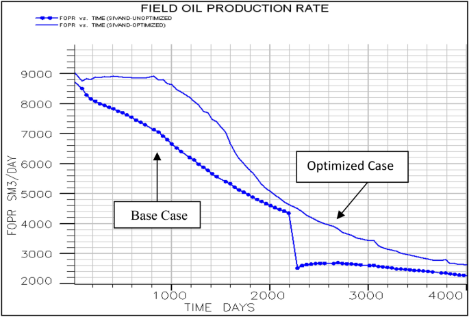

  

  Plot of field oil production rate versus time for the base and optimized cases

  Fig. 12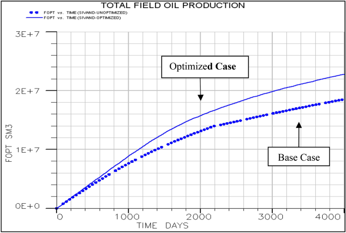

  

  Plot of field total oil production versus time for the base and optimized cases

  Fig. 13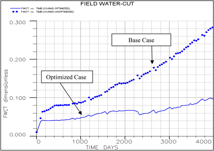

  

  Plot of field water cut versus time for the base and optimized cases

Economic evaluation

We have used the net present value (NPV) to analyze the profitability of the optimization project. NPV is the difference between the present value of cash inflows and the present value of cash outflows over a period of time. A positive NPV indicates that the projected earnings generated by a project or investment exceeds the anticipated costs. It is assumed that an investment with a positive NPV will be profitable, and an investment with a negative NPV will result in a net loss.

The calculated annual NPV over project time for both base and optimized cases is given in Table 10.

Table 10 The annual NPV of base and optimized cases (*M = 1000)

Figure 14 shows the plot of annual NPV versus time for base and optimized cases.

Fig. 14

Plot of annual NPV for base and optimized cases

The results indicate that optimizing the water injection rates will lead to an increase in NPV. The NPV of the base case over project time (from 2020 till 2031) is 18.97 MMM US$ and after optimization it is increased to 24.03 MMM US$. That means water injection optimization will increase the NPV by 21%. It should be mentioned that the NPV was calculated using the cost of a barrel of oil at $46.66. The internal rate of return (IRR) of base case is 234% and that of optimized case is 263%. The IRR is a metric used in financial analysis to estimate the profitability of potential investment. Generally speaking, the higher an internal rate of return, the more desirable an investment is to undertake.

Conclusions

A novel optimization approach is presented in this paper to maximize the recovery factor and sweep efficiency in waterflooding process by determining the optimal water injection rates using streamline simulation. In order to reach a more realistic and practical approach, we have considered both recovery factor and water cut for managing waterfloods.

No new infill water injectors and oil producers are required to increase recovery and sweep efficiency. This methodology can identify producers, which need more injection support and identify injectors, which are not supporting production and contributing to increase water production instead. In addition, it can re-allocate water to injectors supporting low water cut producers.

The proposed approach in this paper is based on the injector/producer pair recovery factors and production well water cuts. An equal or lesser volume of injection water using the optimizer can increase field recovery and decrease field water cut. It can be achieved by changing the choke settings of injectors and producers and therefore no additional investment is required.

This approach is appropriate for full field waterflood optimization with many injectors and producers in high-resolution heterogeneous reservoirs. It has been applied successfully in S field to reduce the field water cut and increase the oil recovery factor and extend the life of the field.

References

Alhuthali AH, Oyerinde D, Gupta AD (2007) Optimal waterflood management using rate control, SPE 102478-PA
Batycky RP (1997) A three-dimensional two-phase field scale streamline simulator, PhD thesis, Stanford university, department of petroleum engineering, Stanford, CA, 6–27
Datta-Gupta A, King MJ (2007) Streamline simulation: theory and practice, 11(4), 87–172, SPE textbook series
Grinestaff GH (1999) Waterflood pattern allocations: quantifying the injector to producer relationship with streamline simulation, SPE 54616
Grinestaff GH, Caffrey DJ (2000) Waterflood management: a case study of the northwest fault block area of Prudhoe Bay, Alaska, Using streamline simulation and traditional waterflood analysis, SPE 63152
Gupta AD (2000) Streamline simulation: a technology update, SPE 65604
Ghori SG, Jilani SZ, Al-Huthali AH, Krinis D, Kumar A (2007) Improving injector efficiencies using streamline simulation: a case study in a giant middle east field, SPE 105393
Ghori SG, Jilani SZ, Vohra IR, Lin C (2006) Improving injector efficiency using streamline simulation: a case study of waterflooding in Saudi Arabia, SPE 93031
Lolomari T, Bratvedt K, Crane M, Milliken WJ, Tyrie JJ (2000) The use of streamline simulation in reservoir management: methodology and case studies, SPE 63157
Naguib M, Sikaiti S, Barrio C, Mahrooqi S, Batycky R (2006) Results of proactively managing a heavy-oil waterflood in south Oman using streamline-based simulation, SPE 101195
Samier P, Quettier L, Thiele M (2001) Applications of streamline simulations to reservoir studies, SPE 66362
Thiele MR, Batycky RP (2003) Water injection optimization using streamline-based workflow, SPE 84080
Acknowledgements
The authors would like to thank IOOC for allowing this work to be published using the S field simulation model and data. Also thanks to Mr. Daneshfar head of reservoir engineering department of IOOC and E. Leung of Schlumberger for their constructive discussions and support.
Funding
No funding for this paper.
Author information
Authors and Affiliations
Corresponding author
Additional information
Publisher's Note
Springer Nature remains neutral with regard to jurisdictional claims in published maps and institutional affiliations.
Rights and permissions
Open Access This article is licensed under a Creative Commons Attribution 4.0 International License, which permits use, sharing, adaptation, distribution and reproduction in any medium or format, as long as you give appropriate credit to the original author(s) and the source, provide a link to the Creative Commons licence, and indicate if changes were made. The images or other third party material in this article are included in the article's Creative Commons licence, unless indicated otherwise in a credit line to the material. If material is not included in the article's Creative Commons licence and your intended use is not permitted by statutory regulation or exceeds the permitted use, you will need to obtain permission directly from the copyright holder. To view a copy of this licence, visit http://creativecommons.org/licenses/by/4.0/.
About this article
Cite this article
Alizadeh, N., Salek, B. Waterflood optimization using an injector producer pair recovery factor, a novel approach. J Petrol Explor Prod Technol 11, 949–959 (2021). https://doi.org/10.1007/s13202-020-01072-3
Received:
Accepted:
Published:
Issue Date:
DOI: https://doi.org/10.1007/s13202-020-01072-3