Application of variance-based sensitivity analysis in modeling oil well productivity and injectivity

Abstract

Well intervention performed on oil or gas well often involves the injection of different stimulating fluids or chemical solutions that aims to increase the production rate. The main objective of this paper is to identify the effect of uncertainty in different variables and parameters used to quantify well productivity and injectivity. Monte Carlo simulation technique is used to develop probabilistic models for radial Darcy’s inflow on the one hand and near wellbore water-based chemical injection on the other hand. The probabilistic model is based on assigning probability density function for all variables and parameters used in the governing formulas. Variance-based sensitivity analysis (VBSA) was performed to quantify the contribution and the correlation between different model’s inputs and outputs. Results indicate that some rough assumptions for about 60% of injectivity model’s parameters and factors, i.e., value with considerable error/uncertainty, can still result in output with small standard deviation in comparison with other parameters. In Darcy’s law, the uncertainty in reservoir pressure value affects the calculated flow rate two times higher than the effect of the formation of permeability or produced fluid viscosity. At low drawdown condition, about 50% of Darcy’s flow variance is caused by the uncertainty in reservoir pressure input value. Throughout VBSA, it is also found that data accuracy of variables and parameters used in the injectivity model is not of importance as for formation permeability, injected fluid viscosity, pressure, and temperature of the injected fluid. Application of this methodology will focus on the cost of information needed by the decision makers and will save a lot of efforts and resources needed to apply confirmation tests or to validate different data sets.

Introduction

For almost all the oil fields around the world, there are essential needs to apply a sort of good treatment from time to time or to apply stimulation techniques to enhance the daily oil production. Acidizing, hydraulic fracturing, solvent injection, chemical water shutoff, cyclic steam stimulation, resin injection, and many other well treatment methods are applied to producing wells. Modeling of the production performance before and after applying well intervention or stimulation treatment will help in the design process of the treatment. Quantification of risks and opportunities associated with the treatment will lead to making the right well intervention or stimulation decision (Devictor 2007).

Once a certain reservoir/well is exposed to production enhancement/stimulation, the next step will be gathering the data. The collected reservoir or well data are always associated with lots of uncertainties. And obviously, acquiring more information will cost time, effort, and resources (Jonkman and Bos 2000). The uncertainties in well and/or reservoir data usually occur because of:

• 1. Having a single-point value for the number of reservoir/well parameters and factors

• 2. Subjective estimation for missing information or data gaps

• 3. Errors in measurements and readings

• 4. Errors in the calculation, especially when using commercial software

• 5. Time factor: values of a lot of reservoir and well-flowing parameters are function of time

• 6. Others, such as human and software errors.

Thus, it is important to evaluate the risk of using uncertain values for some of the variables and parameters used during the screening or designing of a well treatment process.

Monte Carlo simulation, sensitivity analysis, and value of information

Modern engineering design makes extensive use of computer models to test designs before they are manufactured (Rapley 2003). Sensitivity analysis allows designers to assess the effects and sources of uncertainties, in the interest of building robust models (Becker and Rowson 2011). For an engineering model with a number of variables and parameters, it is important to assess input parameters contribute the most to output variability and then assess, if require, additional research to strengthen the knowledge base. It is also useful to assess the parameters that are insignificant and can be eliminated from the final model, thereby reducing the output uncertainty (Chan and Saltelli 1997).

In order to help to analyze decision, results of sensitivity analysis should be quantitative rather than qualitative to enable meaningful comparisons and the desired sensitivity analysis method should be independent of model assumptions (McNamee and Celona 2008).

In probability theory and statistics, variance measures how far a set of numbers are spread out around the average value of a variable (Loeve 1977). Variance-based sensitivity analysis (VBSA) is a form of global sensitivity analysis. When a certain problem is modeled in a probabilistic framework, i.e., inputs are given in terms of ranges or probability distribution curves, VBSA decomposes the variance of the output of the model into fractions which can be attributed to inputs. For example, given a model with two inputs and one output, one might find that 80% of the output variance is caused by the variance in the first input and 20% by the variance in the second. These percentages are directly interpreted as measures of sensitivity (Sobol 2001).

The VBSA methods are model free and do not assume substitute functional relationship for the model under investigation unlike regression and correlation-based method (Mollaei and Lake 2011). Therefore, VBSA methods are suitable for the sensitivity analysis of well injectivity and productivity-complicated models. VBSA is conducted through four steps (Chan and Saltelli 1997):

• 1. Building a computational model and defining its input and output variable(s),

• 2. Defining uncertainty ranges and assigning probability density functions to each input variable,

• 3. Using random sampling method (as for Monte Carlo simulation) and generating an input matrix and evaluating the output, and

• 4. Assessing the influences of each input variable on the output

Monte Carlo simulation is a well-known numerical modeling technique. This technique uses random numbers that are generated within a selected probability distribution model and can have upper and lower limits for an uncertain variable (model input) (Sarmiento and Steingrímsson 2007). Monte Carlo simulation represents uncertainty surrounding all possible incomes and outcomes for various options by setting probabilistic distributions for each of the inputs. The probabilistic distribution or density function that will be assigned to each input depends on the margin of error of obtained data input.

Utilizing Monte Carlo simulation allowed us to apply VBSA for all variables included in the mathematical formulae used for the design of well treatment (well injectivity and productivity). The results of VBSA showed the effect of each variable on the final output. Quantifying this effect by applying different value ranges and different probability distributions to each variable and recording the outcomes for each simulation run gives a clear ranking to the studied variables in terms of contribution to the output’s variance as a result from applying VBSA. This ranking has a direct impact on future decisions that are related to data collection and the application of different methodologies to obtain an accurate value of each variable (Hanssensvei), i.e., value of information (VOI). VOI is the main concern in technical decision making, especially for variables related to pressures, reservoir’s fluids, and rock properties. That is because of the high costs encountered in each of the well operation or laboratory test needed to obtain or verify the numerical value of each variable (Bratvold 2010).

Therefore, VOI can be achieved and benefited through the application of VBSA on a known model that can help to reduce the uncertainty of output results significantly by reducing the uncertainty of the input parameters that cause the largest uncertainty. This is applied to a simple well treatment model, in which hypothetical data were used for different uncertainty ranges. Decision analysis process based on VOI obtained through the VBSA is developed for a well treatment design, which may include injection of fluids into a well and then back-production from the same well as the case for many stimulation treatments. Figure 1 shows the newly developed procedure to help in undertaking well stimulation technical decision. This procedure includes the following steps:

Fig. 1

Contribution of the probability-based modeling approach to the process flow of a well treatment

• 1. To develop a simple screening model using probability-based inputs

• 2. To apply the VBSA on the screening model using Monte Carlo simulation

• 3. Determination of variables that have a high impact on the design model’s outcomes (VOI): this was obtained for both models by ranking the contribution of the input data to the model’s outputs calculated variance

• 4. Data validation: once the uncertain parameters that highly affect the output were defined then it is important to find out clear-cut values of those parameters before applying them in a deterministic treatment design model.

Injectivity and productivity models

For an oil well completed in a number of layers/formations, the following models were created to simulate the well treatment in terms of injection of water-based chemical solution and oil production afterward:

• 1. Fluid injectivity: where it is required to estimate the penetration or invasion depth into all opened zones. The complexity of this issue comes when the fluid injection is bullheaded in multilayer reservoir, i.e., no zone isolation is applied. Bullhead injection of well stimulation fluid is considered a cost-effective operational method, in which the treatment fluid(s) is injected in all opened zones without zone isolation. A simple analytical model, using Microsoft Excel and Monte Carlo simulation, was developed to calculate and to illustrate the radial invasion of a stimulation fluid(s) into all opened zones. The model also calculates the injected fluid volume in each zone. It also predicts the fluid injection rate in each opened zone provided that reservoir data are available and correct. During the bullhead injection process into multi-opened zones, the radius of fluid invasion or penetration into each zone can be determined by normalizing all invasion radii to the maximum designed invasion radius, r_max. This can be done by pre-defining the value of r_max as in the following developed expression based on Darcy’s flow: equation:

  $$\frac{{r_{j} }}{{r_{ \hbox{max} } }} = \sqrt {\frac{{k_{j} \left( {P_{i} - P_{j} } \right) \cdot \varphi_{{j{ \hbox{max} }}} \cdot \left( {1 - s_{{or\;j{ \hbox{max} }}} } \right) \cdot \ln \left( {\frac{{r_{ \hbox{max} } }}{{r_{w} }}} \right)}}{{k_{{j{ \hbox{max} }}} \left( {P_{i} - P_{{j{ \hbox{max} }}} } \right) \cdot \varphi_{j} \cdot \left( {1 - s_{{{\text{or}}\;j}} } \right) \cdot \ln \left( {\frac{{r_{j} }}{{r_{w} }}} \right)}}} ,$$

  (1)

  where r_j is the injected fluid invasion radius in layer j, k is the formation permeability, P_i is the injection pressure, $P_{j}$ is the reservoir pressure, r_w is wellbore radius, s_or is the residual oil saturation, and φ is the formation porosity.

  In order to determine the $\left( {j{ \hbox{max} }} \right)$ layer, a [$k_{j} \cdot \left( {P_{i} - P_{j} } \right)/\varphi_{j} ]$ function is created based on the contribution of each parameter in the calculation of each $r_{j}$. It was found that for any bullhead liquid injection in the multilayered reservoir, the deepest penetration occurs in the layer which has the lowest formation pressure and the highest permeability.

• 2. Temperature distribution within the fluid-invaded area: since the injected fluid will gain the reservoir heat during the injection process. Injected fluid temperature should be modeled while considering the fact that fluid temperature plays the main role in scheming chemical reaction during the injection process. Bullhead injection of any fluid into the reservoir will temporarily cool down the wellbore vicinity. Modeling such cooling effect is useful when it comes to designing well shut-in/soak period and/or chemical gelation time for well treatment using, for instance, polymer or x-linked polymer placement. The cooled area around the wellbore due to heat transfer between the relatively low temperature T_i of the injected fluid with injection rate (i) and the high temperature of the reservoir formation T_j at time t can be modeled based on Marx and Langenheim (1959) model as:

  $$A_{c} = \frac{{ - \left( {i_{j} \cdot \rho_{i} \cdot C_{Pi} \cdot T_{i} } \right) \cdot M_{j} \cdot h_{j} }}{{4\left( {T_{i} - T_{j} } \right)\alpha_{j} \cdot M_{s}^{2} }} \cdot \left\{ {e^{{\left( {4(M_{s} /M_{j} ) ^{2} \left( {\alpha_{j} /h_{j}^{2} } \right) \cdot t} \right)}} erfc\left( {\sqrt {\left( {4(M_{s} /M_{j} ) ^{2} \left( {\alpha_{j} /h_{j}^{2} } \right) \cdot t} \right)} } \right) + 2\sqrt {\frac{{\left( {4(M_{s} /M_{j} ) ^{2} \left( {\alpha_{j} /h_{j}^{2} } \right) \cdot t} \right)}}{\pi }} - 1} \right\}$$

  (2)

  where A_c is the cooled area around the wellbore, ρ_i is the injected fluid density, Mj is the volumetric heat capacity for reservoir’s invaded layer j, α is the thermal diffusivity, h is the layer thickness, and C_p is the specific heat of the injected fluid.

• 3. Chemical concentration changes during the injection process (dilution): this is necessary to be understood in order to estimate the chemical reaction in any position around the wellbore and deeper. The target of this section is to build a simple model that illustrates the concentration distribution of the dissolved chemicals x in water-based solution at any distance from the wellbore during its injection into reservoir formation layer with irreducible water saturation S_wi.

  $$[x] = \left\{ {\begin{array}{*{20}l} {\left[ x \right]_{i} \left( {1 - \frac{{s_{wi} \cdot r^{2} }}{{\left( {1 - s_{or} } \right)r_{i}^{2} + s_{wi} \cdot r^{2} }}} \right)} \hfill & {{\text{if}}\;\left( {r_{w} \le r \le r_{j} } \right)} \hfill \\ 0 \hfill & {{\text{if}}\;(r > r_{j} )} \hfill \\ \end{array} } \right..$$

  (3)

  Equation 3 models the volumetric chemical dilution during injection in porous media without considering retention of chemicals during its invasion into the information layers.

  The combination of fluid injectivity model, temperature distribution model, and chemical dilution model can give a better prediction to the reaction kinetics at any point inside multilayered formation during and after the injection process.

• 4. Inflow performance using Darcy’s law(Joseph 1985) for steady-state radial flow $q_{j}$ and skin factor s.

  $$q_{j} = \frac{{k_{j} h_{j} \left( {P_{i} - P_{j} } \right)}}{{141.2 B\mu \left( {ln\frac{{r_{e} }}{{r_{w} }} + s} \right)}}$$

  (4)

The injectivity and productivity models have got many variables and parameters as shown in the equations from 1 to 4. Uncertainties are associating with all these variables. Modeling these equations stochastically, i.e., by assigning probability distribution function for the inputs (with different ranges of possible errors: minimum and maximum), will allow us to apply the VBSA method.

Many calculation trials and scenarios were performed using data from the literature in which:

• 1. All inputs are assumed as a range of values between the minimum and maximum limits (uniform probability distribution), and then the VBSA is applied on the output

• 2. All inputs are given a mean value, minimum and maximum values (triangular or beta PERT probability distributions), and then the VBSA is applied and results are recorded

• 3. Different probability density functions are assigned to the inputs, and the VBSA is applied on the output and compared with the two previous scenarios.

• 4. The range between the minimum and maximum limits for each input was changed from ± 3% to ± 50% from the mean value, and the VBSA is applied on the outputs and compared for all previous scenarios.

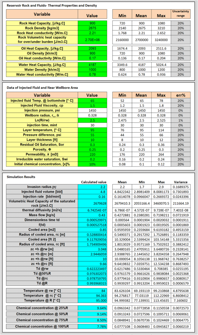
Two spreadsheet examples for injectivity and productivity calculation with different uncertainty ranges and PDFs are illustrated in Appendix 1, in which the source of data is from a Sudanese oil well.

VBSA results

Throughout the sensitivity analysis, it is found that residual oil saturation has a minor effect on the injected fluid invasion radius, while porosity, permeability, injected fluid viscosity, and pressure difference (between injection pressure and formation pressure) are all important to determine accurate penetration depth of the injected fluid into any opened zone. Although porosity value is important in the injected pore volume calculation, the flushing radius or fluid’s invasion/penetration depth into the formation must be calculated first in order to determine the injected pore volume in each layer for bullheading well treatment. Figure 2 illustrates the relationship between the inputs and the invasion radius (Ri) in terms of correlation and inputs contribution to Ri variance.

Fig. 2

Sensitivity analysis on the injected fluid radius in a pay zone

However, when the VBSA was performed for the calculated injected fluid volume, it was found that it is highly affected by the uncertainties in values of pay zone thickness, injected fluid viscosity, and formation permeability.

Heat transfer during the injection process from the hot formation to the relatively cold injecting fluid was modeled as per equation 2. From the results of sensitivity analysis, it was found that the value of the injected fluid temperature at any point in the reservoir mainly depends on the initial formation temperature, and therefore, the uncertainty in the other variables, i.e., rock and reservoir fluids’ heat capacity and conductivity, is not contributing to the calculated cooled zone around the wellbore during the injection, as shown in Fig. 3.

Fig. 3

Contribution of inputs (assumptions) on the variance of the calculated cooled area around the wellbore during stimulation fluid injection

In addition, the VBSA indicates also that the calculated chemical concentration at any point around the wellbore is mainly affected by the value of the initial chemical concentration. However, this value can also be affected by the uncertainties in the calculated fluid penetration radius but not with irreducible water saturation and residual oil saturation as shown in Fig. 4.

Fig. 4

Sensitivity analysis on the injected chemical concentration at different positions from the wellbore

On the other hand, the results of VBSA on Darcy’s flow indicate the importance of having accurate reservoir pressure data since the calculated production rate is highly sensitive to pressure in comparison with permeability, formation volume factor, and viscosity values, i.e., the uncertainty in reservoir pressure value affects the flow rate calculation and results in two times higher than the effect of the formation permeability or produced fluid viscosity. Uncertainty in the values of drainage radius or skin factor slightly affects the calculated production rate as shown in Fig. 5.

Fig. 5

VBSA on Darcy’s flow

In order to correlate the relationship between all possible uncertainty ranges of reservoir pressure and Darcy’s flow variance, the ratio between drawdown and reservoir pressure (ΔP/Pr) is plotted versus Darcy’s flow variance as illustrated in Fig. 6. For low drawdown, the calculated/modeled flow rate is very sensitive to uncertainty in reservoir pressure value (about 50% of Darcy’s flow variance is caused by uncertainty in reservoir pressure value).

Fig. 6

Sensitivity of reservoir pressure and drawdown on Darcy’s flow variance

In summary, the VOI of the following variables is higher than other variables as per the models above:

• 1. Injected fluid temperature calculated/measured downhole: this variable is mainly dependent on two factors, which are fluid’s surface temperature and geothermal gradient. Accurate information about these factors is easy to obtain.

• 2. Injected fluid viscosity: this variable can be modeled via laboratory tests in which the viscosity is measured at different temperatures and shear rates.

• 3. Layer’s temperature: it is better to be measured rather than making rough estimation using geothermal gradient

• 4. The pressure difference between the injected fluid and the pore pressure: the value of this variable must carefully be determined through calculations and measurement. Cross-checking of the calculated values of the pressure is highly recommended

• 5. Layer thickness: it is very important to determine the accurate value for this factor when it comes to the estimation of total treatment fluid’s volume.

• 6. Porosity: although precise information about formation porosity is not important for the estimation of the temperature and chemical concentration profiles around the wellbore, it is important for the calculation of the fluid invasion radius.

• 7. Permeability: an accurate value of the effective permeability is highly considered for the calculation of the invaded area and the injected fluid’s volume. Laboratory tests are required to estimate the relative permeability versus saturation as well as the rock’s absolute permeability. Inaccurate value of the effective permeability will be vulnerable for the outcome of the entire injectivity simulation, which is not the case for well productivity models.

• 8. Initial chemical concentration in the injected fluid: it is a designing variable; therefore, it should be carefully determined.

• 9. Reservoir pressure and drawdown: although oil production rate is a function of many variables and factors, it is very sensitive to pressure value and its uncertainty range.

In addition, simulation trails on the productivity probabilistic model indicated that probability density function assigned to model’s input variables has a limited effect on the outcomes in terms of sensitivity to output variance. It is also found that increasing the uncertainty ranges given to the model’s input from ± 3% to ± 30% has a trivial effect on the VBSA on the calculated flow rate (see the “Appendix” section).

Benefits of data validation using probability-based models

The expected benefits of data validation using the VBSA for operating companies, service companies, and engineering consultant are compiled in Table 1.

Table 1 Technical and commercial benefits of utilizing the VBSA in both design and operational activities

Conclusion

• 1. Quantified VOI can be obtained by applying the VBSA on a known model, such as Darcy’s flow or injectivity model, and thus we can reduce the uncertainty of the model’s output significantly by reducing the uncertainty of the input parameters that cause the largest uncertainty.

• 2. A simple model, using Microsoft Excel and Monte Carlo simulation, is developed to calculate and illustrate injection fluid invasion into all opened zones. The model also calculates the injected fluid volume in each zone. It also predicts the fluid injection and production rate in and from each opened zone. Heat transfer during the injection process from the hot formation to the cold injecting fluid is modeled. In other words, the cooling effect of the injected fluid in a radial and a vertical direction is simulated for every invaded zone, in which the cooled radius and the cooled thickness are estimated during the fluid injection process. In addition, an equation is developed to simulate the dilution process of dissolved chemicals in water-based solution during the invasion of the solution fluid into the reservoir formation layer.

• 3. The combination of fluid injectivity model, temperature distribution model, and chemical dilution model can give a better prediction to the reaction kinetics at any point inside the multilayered formation during and after the injection process. However, the effect of data accuracy of many variables and parameters used in the injectivity model is found to be less important compared to injected fluid’s temperature, viscosity, chemical concentration, and pressure. Uncertainty in heat capacities and fluids saturations values for each formation layer has a very limited effect on temperature profile around the well during the injection.

• 4. Modeled production rate based on steady-state radial Darcy’s flow is found to be highly sensitive to formation pressure in comparison with permeability, formation volume factor, and viscosity values. Uncertainty in the values of drainage radius or skin factor slightly affects the calculated production rate.

• 5. Simulation trails on the productivity probabilistic model indicated that probability density function assigned to model’s input variables has a limited effect on the outcomes in terms of sensitivity to output variance. It is also found that increasing the uncertainty ranges given to model’s input from ± 3% to ± 30% has a trivial effect on the VBSA on the calculated flow rate.

• 6. A lot of technical benefits and cost-effectiveness can be achieved by applying the VBSA on probability-based models for future well stimulation treatments in petroleum operating companies, service companies, and consultants.

Appendix

• 1. Injectivity spreadsheet example

  

• 2. Production forecast example based on Darcy’s radial flow

References

Becker W, Rowson J (2011) Bayesian sensitivity analysis of a model of the aortic valve. J Biomech 44(8):1499–1506
Bratvold MG (2010) Probabilistic modeling for decision support in integrated operations. In: SPE 127761
Chan K, Saltelli A (1997). Sensitivity analysis of model output: variance-based methods make the difference. In: Winter simulation conference, European Commission Joint Research Centre, Italy, pp 261–268
Devictor N (2007) Advances in methods for uncertainty and sensitivity analysis. Commissariat à l’Energie Atomique (CEA)
Jonkman RK, Bos C (2000) Best practices and methods in hydrocarbon resource estimation, production and emission forecasting, uncertainty evaluation and decision making. In: SPE European petroleum conference, Paris, France: SPE 65144
Joseph JA (1985) Unsteady-state spherical flow with storage and skin. Soc Petrol Eng
Loeve M (1977). Probability theory. In: Graduate texts in mathematics, 4th ed., vol. 45. Springer, Berlin, p 12
Marx JW, Langenheim RH (1959). Reservoir heating by hot fluid injection. In: SPE 1266-G
McNamee P, Celona J (2008) Decision analysis for the professional (fourth edition ed). SmartOrg, Inc
Mollaei A, Lake LW (2011) Application and variance based sensitivity analysis of surfactant-polymer flooding using modified chemical flood predictive model. J Petrol Sci Eng 79(1–2):25–36
Rapley LV (2003) Decision and risk analysis tools for the oil and gas industry. In: SPE Eastern Regional/AAPG. SPE, Pennsylvanla
Sarmiento ZF, Steingrímsson B (2007) Computer programme for resource assessment and risk evaluation using Monte Carlo simulation. LaGeo S.A. de C.V. and Unite Nation University, Zosimo
Sobol I (2001) Global sensitivity indices for nonlinear mathematical models and their Monte Carlo estimates. Math Comput Simulat 55(1–3):271–280
Author information
Authors and Affiliations
Corresponding author
Additional information
Publisher's Note
Springer Nature remains neutral with regard to jurisdictional claims in published maps and institutional affiliations.